A new rolling tachyon solution of cubic string field theory

      

City, University of London Institutional Repository

Citation

:

Forini, V., Grignani, G. & Nardelli, G. (2005). A new rolling tachyon solution of cubic string field theory. Journal of High Energy Physics, 2005, 079.. doi: 10.1088/1126-6708/2005/03/079

This is the published version of the paper.

This version of the publication may differ from the final published

version.

Permanent repository link:

http://openaccess.city.ac.uk/19746/

Link to published version

:

http://dx.doi.org/10.1088/1126-6708/2005/03/079

Copyright and reuse:

City Research Online aims to make research

outputs of City, University of London available to a wider audience.

Copyright and Moral Rights remain with the author(s) and/or copyright

holders. URLs from City Research Online may be freely distributed and

linked to.

City Research Online: http://openaccess.city.ac.uk/ [email protected]

Journal of High Energy Physics

A new rolling tachyon solution of cubic string field

theory

To cite this article: Valentina Forini et al JHEP03(2005)079

View the article online for updates and enhancements.

Related content

Taming the tachyon in cubic string field theory

Erasmo Coletti, Ilya Sigalov and Washington Taylor

-Disk partition function and oscillatory rolling tachyons

Niko Jokela, Matti Järvinen, Esko Keski-Vakkuri et al.

-On tachyon condensation and open-closed duality in the cstring theory

Jörg Teschner

-Recent citations

Nonlocal gravity and the diffusion equation

Gianluca Calcagni and Giuseppe Nardelli

-String field theory: From high energy to cosmology

I. Ya. Aref’eva

-String theory as a diffusing system

-JHEP03(2005)079

Published by Institute of Physics Publishing for SISSA

Received:February 17, 2005 Revised: March 23, 2005 Accepted: March 30, 2005 Published:May 4, 2005

A new rolling tachyon solution of cubic string field

theory

Valentina Forini∗

Dipartimento di Fisica and I.N.F.N. Gruppo Collegato di Trento Universit`a di Trento, 38050 Povo (Trento), Italia

E-mail: [email protected]

Gianluca Grignani†

Dipartimento di Fisica and Sezione I.N.F.N.

Universit`a di Perugia, Via A. Pascoli I-06123, Perugia, Italia E-mail: [email protected]

Giuseppe Nardelli‡

Dipartimento di Fisica and I.N.F.N. Gruppo Collegato di Trento Universit`a di Trento, 38050 Povo (Trento), Italia

E-mail: [email protected]

Abstract:We present a new analytic time dependent solution of cubic string field theory at the lowest order in the level truncation scheme. The tachyon profile we have found is a bounce in time, a C∞ function which represents an almost exact solution, with an extremely good degree of accuracy, of the classical equations of motion of the truncated string field theory. Such a finite energy solution describes a tachyon which at x0 _{= −∞} is at the maximum of the potential, at later times rolls toward the stable minimum and then up to the other side of the potential toward the inversion point and then back to the unstable maximum forx0 →+∞. The energy-momentum tensor associated with this rolling tachyon solution can be explicitly computed. The energy density is constant, the pressure is an even function of time which can change sign while the tachyon rolls toward the minimum of its potential. A new form of tachyon matter is realized which might be relevant for cosmological applications.

Keywords: Tachyon Condensation, String Field Theory.

∗_{Work supported by INFN of Italy.}

JHEP03(2005)079

Contents

1. Introduction 1

2. The rolling tachyon solution in cubic string field theory 4

3. Energy-momentum tensor 10

4. Conclusions 14

1. Introduction

In recent years there has been great progress, particularly due to Sen, in our understanding of the role of the tachyon in string theory (see [1] with references to earlier works). The basic idea is that the perturbative open string vacuum is unstable but there exists a stable vacuum toward which a tachyon field naturally moves.

String theory must eventually address cosmological issues and hence it is crucial to understand the role of time dependent solutions of the theory. The rolling tachyon [2] is an example of such a solution and in fact it has been applied to the study of tachyon driven cosmology, cosmological solutions describing the decaying of unstable space filling D-branes [3, 4]. In the decay, the energy density remains constant and the pressure approaches zero from negative values as the tachyon rolls toward its stable minimum. This form of tachyon matter could have astrophysical consequences and it then seems of utmost importance to confirm its existence using string field theory.

JHEP03(2005)079

The direct approach based on the analysis of the classical equations of motion of bosonic open string field theory (cubic string field theory, CSFT [9]) is generally believed to be equivalent to the approach based on two dimensional conformal field theory. This equivalence is however less than manifest also because it is not yet known a satisfactory rolling tachyon solution of the cubic string field theory equations of motion even at the classical level and at the lowest order, the (0,0), in the level truncation scheme [10, 11]. In this paper we solve this problem providing a well behaved (almost exact) time dependent solution of the lowest order equations of motion of cubic string field theory. At this order one considers only the tachyon field and the cubic string field theory action becomes

S= 1

g2 o

Z

d26x

µ

1

2t(x) (¤+ 1)t(x)− 1 3λc

³

λ(1_c/3)¤t(x)´3

¶

, (1.1)

where the coupling λchas the value

λc=

39/2

26 = 2.19213. (1.2)

Considering spatially homogeneous profiles of the formt(x0), wherex0is time, the equation of motion derived from (1.1) is

(∂2₀₋1)t(x0) +λ1−∂20/3

c

³

λ−∂20/3

c t(x0)

´2

= 0. (1.3)

We have found an almost exact analytic solution of this equation, which is given by the following well defined integral 1

t(x0) = 9λ

−5/3 c

4√πlogλc

Z _∞

0

dτ¡1₋2τ2¢e−τ2loghcoshx0+ cos(4τplogλc/3)

i

. (1.4)

Being the equation of motion time reversal invariant, the solution (1.4) is a symmetric bounce in x0, a C∞ function with the appropriate boundary conditions to describe a rolling tachyon. Such a constant energy density solution, in fact, describes a tachyon which at x0 _{= −∞ is at the maximum of the potential, at later times rolls toward the} stable minimum and then up to the other side of the potential toward the inversion point and then back to the unstable maximum forx0_{→ ∞}.

If the decaying D-brane is coupled to closed strings it will act as a source for closed string modes [12 – 14]. A rolling tachyon is a time dependent source which will produce closed string radiation. All the energy of the D-brane will eventually be radiated away into closed strings. In the classical rolling tachyon picture described above this would correspond to the introduction of a friction that would eventually stop the rolling tachyon at the minimum of its potential.

The profile (1.4) does not present all the cumbersome features found in previous works on rolling tachyons in cubic string field theory, like ever growing oscillations with time and an energy-momentum tensor that cannot be derived [15, 16, 11, 17]. For the tachyon profile (1.4) in fact the associated energy-momentum tensor can be computed explicitly.

JHEP03(2005)079

The energy density E is constant while the pressure p(x0) is an even function of time. Pressure and energy density depend on an arbitrary constant (the constant up to which the action is defined) and they can be chosen for example in such a way that the Dominant Energy Condition,E ≥ |p(x0)|, holds at any instant of time. In this case the pressurep(x0) starts negative when the tachyon is at the unstable maximum of the potential, at later times becomes positive, while the tachyon reaches the minimum of the potential, and finally it goes back to its negative starting value atx0 = +∞. By choosing the initial energy density to be higher, however, one might even realize the situation in which the tachyon reaches the minimum of its potential when its pressure vanishes. The rolling tachyon matter associated to the solution has in this case an interesting equation of state p(x0) = wE, withw that smoothly interpolates between₋1 and 0, while the tachyon moves from the maximum of its potential to the minimum [18]. Passed this time, however, the pressure becomes positive until the tachyon goes again through its minimum. This form of tachyon matter is thus different to the one described in [18, 8, 19].

In boundary string field theory and in most of the models used to study tachyon driven cosmology, the stable minimum of the potential is taken at infinite values of the tachyon field [20 – 22, 18, 8, 19]. The tachyon thus cannot roll beyond its minimum. One of the main objections to the rolling tachyon as a mechanism for inflation is that reheating and creation of matter in models where the minimum of the potential is at T _{→ ∞} is problematic because the tachyon field in such theory does not oscillate [23, 3]. In cubic string field theory the naive value of the minimum of the potential is at finite values of the tachyon field2. Therefore, the coupling of the free theory to a Friedman-Robertson-Walker metric [3], and the consequent inclusion of a Hubble friction term, might lead from the classical solution (1.4) to damped oscillations around the stable minimum of the potential well. Cubic string field theory might then open new perspectives in tachyon cosmology.

It is also possible, however, that a true solution of the complete cubic string field theory without the level approximation would be non-oscillating, like Sen’s rolling tachyon solution. In fact the inclusion of higher level fields might change the interactions in such a way that even if the minimum of the potential would stay at finite values of the tachyon field the rolling tachyon solution would not have oscillations about it, but would just reach the minimum of the potential at infinite times. As we shall show also for the solution (1.4) the tachyon rolls from the top of the potential towards the stable minimum and then up to the other side, but the inversion point is lower then the maximum of the potential. This is because the cubic term in the interaction is dressed by a kinematical factor depending on the tachyon field derivatives.

The paper is organized as follows. In section 2 we derive the solution (1.4) and discuss its analytical properties. In section 3 we compute the associated energy momentum tensor, study its time dependence and discuss the tachyon matter it describes. In the conclusions we outlook some possible checks and applications of the new rolling tachyon solution of cubic string field theory.

2_{By “naive” we mean that a field redefinition could always map the minimum of the potential at infinity,}

JHEP03(2005)079

2. The rolling tachyon solution in cubic string field theory

The action of cubic open string field theory reads [9]

S=− 1 g2 o

Z µ

1

2Φ·QBΦ + 1

3Φ·(Φ∗Φ)

¶

, (2.1)

where QB is the BRST operator, ∗ is the star product between two string fields and Φ is the open string field containing component fields which correspond to all the states in the string Fock space. If we consider only the tachyon field t(x) in Φ, |Φi=b0|0it(x), the action (2.1) becomes (1.1). For profiles that only depend on the time x0 the equation of motion derived from (2.1) is (1.3) and we shall now look for a solution to that equation. Our procedure is based on the idea that eq. (1.3) can be generalized to become a non-linear differential equation with an arbitrary parameterλwhich substitutes the fixed value (1.2)

(∂2₀₋1)t(x0) +λ1−∂20/3

³

λ−∂20/3_t(x0₎

´2

= 0. (2.2)

Then λ can be treated as anevolution parameter. Fixing the initial value λ= 1 one can easily find an exact solution to (2.2) and then one can study how this solution evolves to different values ofλkeeping its property of being a solution of (2.2). We shall find that the equation governing the evolution inλis extremely simple and we shall look for a solution of (2.2) for generic λ, setting eventuallyλ=λcas in (1.2).

Whenλ= 1, eq. (1.3) admits a particularly simple exact solution, the following bounce

t(logλ= 0, x0) = 3

2cosh2(x0_/2) = 6

Z _∞

0

τcos(τ x0)

sinh(πτ) dτ . (2.3)

The boundary conditions of (2.3) are such that∂t(0, x0_)/∂x0 _{= 0 at x}0 _=±∞.

Now we shall interpret the solution (2.3) as the “initial” condition of an “evolution” equation with respect to the “time” logλ. To find how the solution evolves we shall have to provide a careful treatment of infinite derivative operators of the type

q∂2 =elogq ∂2 _≡

∞ X

n=0

(logq)n

n! ∂

2n_{, (2.4)}

which act on the function t(x0) in (2.2) when λ₆= 1. These operators play a crucial role in string field theories and related models. We shall thus provide a possible solution to the long standing problem of how to treat this infinite derivative operators in string field theory.

A particularly convenient redefinition of the tachyon field that leaves invariant the initial condition (2.3) is

T(logλ, x0) =λ5/3+∂02/3_{t(logλ, x}0_{). (2.5)}

With this field redefinition eq. (1.3) transforms into the following

(∂2₀₋1)T(logλ, x0) +λ−2/3³λ−2∂02/3_{T(logλ, x}0₎

´2

JHEP03(2005)079

Since the operator λ−2∂02/3 is defined as a power series of logλ through eq. (2.4), it is natural to look for solutions of eq. (2.6) of the form

T(logλ, x0) =

∞ X

n=0

(logλ)n

n! tn(x

0_{). (2.7)}

It is not difficult to check that at any desired order n in (2.7) the functions tn(x0) can

always be written as finite sums of the form

tn(x0) = n

X

k=0

a(_kn)

cosh2k+2(x0_/2), (2.8)

and the differential equation for the tachyon field becomes an algebraic equation for the unknown coefficients a(_kn). Thus, an exact solution of (2.6) can always be obtained as a series representation. However, in order to obtain solutions preserving the correct boundary conditions, it is mandatory to look for solutions that, although approximate, sum the whole series (2.7) rather than to find the exact coefficients a(_kn) at any fixed truncation

n of the sum (2.7). In fact, it is easy to show that any truncation of the sum (2.7) leads to solutions with wild oscillatory behavior with increasing amplitudes, whose physical meaning is difficult to interpret. Only the resummation of the whole series smoothens such oscillations.

A more convenient representation oftn(x0) alternative to (2.8) is given by

tn(x0) = 6

Z _∞

0

τcos(τ x0₎

sinh(πτ) Pn(τ)dτ , (2.9)

Pn(τ) being a polynomial of even powers of τ of degree 2n. This representation is

par-ticularly useful since it provides the tn(x0) in terms of eigenfunction of the operator ∂02. The field redefinition (2.5) was chosen in such a way that the form of the coefficients (2.9) becomes particularly simple, so simple that the series (2.7) can be resummed. Requiring that the profile (2.7) satisfies the boundary conditions ∂T(0, x0)/∂x0 = 0 at x0 =±∞ as in (2.3) and that it is a very accurate approximate solution of the equation of motion (2.6), fixes the polynomials Pn(τ) to be of the form

Pn(τ)'τ2n. (2.10)

This leads to the following approximate solution of eq. (2.6)

T(logλ, x0) = 6

Z _∞

0

τcos(τ x0₎ sinh(πτ) e

logλ τ2

dτ = 6λ−∂02

Z _∞

0

τcos(τ x0₎

sinh(πτ) dτ , λ <1. (2.11)

Note that all the λ-dependence in (2.11) is encoded in the operator λ−∂02 acting on the solution of eq. (2.6) withλ= 1. In factT(logλ= 0, x0)≡t(logλ= 0, x0) and λ−∂02 plays the role of the “evolution” operator (with respect to the “time” logλ) acting on the initial condition T(logλ= 0, x0_),

JHEP03(2005)079

Clearly, the representation (2.11) of the solution T(logλ, x0) is valid only for λ ∈ (0,1]. In our case the physically relevant value of λ is the one given in (1.2), which is greater than one. Consequently, we need an analytical continuation of the representation (2.11) to positive values of logλ.

Eq. (2.11) shows that the evolution of the tachyon field with respect to the parameter logλ is simply driven by the diffusion equation with (negative) unitary coefficient. In fact (2.11) satisfies the diffusion equation

∂T(logλ, x0)

∂logλ =−

∂2T(logλ, x0)

∂(x0₎2 (2.13)

with respect to the “time” variable logλ and the “space” variable x0_{, with “initial” and} “boundary” conditionsT(0, x0) = 3/[2cosh2(x0/2)], T(logλ,±∞) = 0.

Now we face the problem of the analytical continuation of the representation (2.11) to positive values of logλ. Setting τ =−isin eq. (2.11), we rewrite T as

T(logλ, x0) = 3

iλ

−∂2 0

Z +i∞

−i∞

sesx0

sin(πs)ds . (2.14)

In eq. (2.14) the integral can be closed with semi-circles at infinity to the right or to the left depending on the sign ofx0. Let us choose for instancex0 <0. Then (2.14) reads

T(logλ, x0 <0) =₋6λ−∂02

∞ X

n=1

(₋1)nnenx0. (2.15)

In eq. (2.15) one would be tempted to replace the operator λ−∂2

0 with its eigenvalue λ−n2 inside the series, namely

−6

∞ X

n=1

(₋1)nλ−n2nenx0, λ >1, (2.16)

thus providing very easily the required analytical continuation to the regionλ >1. However this procedure is incorrect. This is an important point, as the solutions in cubic string field theory (CSFT) analyzed in the recent literature [11] have precisely the form (2.16). A cavalier treatment of the infinite derivative operator λ−∂02, however, might lead to the wrong conclusion that no rolling tachyon solutions exist in CSFT.

JHEP03(2005)079

Another argument which can be given to understand why (2.16) does not reproduce the tachyon field forλ >1 is the following. Eq. (2.11) is manifestly even, and then all its odd derivatives must vanish at the originx0 _{= 0}3_{. This is not true for the representation (2.16).} A possible way to overcome these difficulties, and thus to solve the problem of how infinite derivative operators of the type λ−∂02 can be treated, is through a Mellin-Barnes representation for the operator λ−∂2

0,

λ−∂20 =

∞ X

n=0

(₋logλ)n n! ∂

2n 0 =

1 2πi

Z γ+i∞

γ−i∞

dsΓ(₋s)(logλ)s∂₀2s, Reγ <0. (2.17)

Acting with (2.17) in (2.15), we find

T(logλ, x0 <0) = ₋3

πi

Z γ+i∞

γ−i∞

dsΓ(₋s)(logλ)s

∞ X

n=1

(₋1)nn2s+1enx0

= 3e

x0

πi

Z γ+i∞

γ−i∞

dsΓ(−s)(logλ)sΦ(−ex0,−2s−1,1)

= 12e

x0

√ πi

Z γ+i∞

γ−i∞

ds (4 logλ) s

Γ(−s−1/2)

Z _∞

0 dt t2

t−2s ex0

+et , (2.18)

where Φ is the Lerch Transcendent defined as

Φ(z, s, v) =

∞ X

n=0

(v+n)−szn, _|z_|<1, v₆= 0,₋1,₋2, . . .

= 1

Γ(s)

Z _∞

0

dt t

s−1_e−(v−1)t

et_−z , (2.19)

and the last equation in (2.18) follows from the integral representation of Φ given in (2.19). The gamma function in (2.18) can be rewritten by using the formula

1

Γ(₋s₋1/2) = 1 2πi

Z

C

dz ezzs+1/2 (2.20)

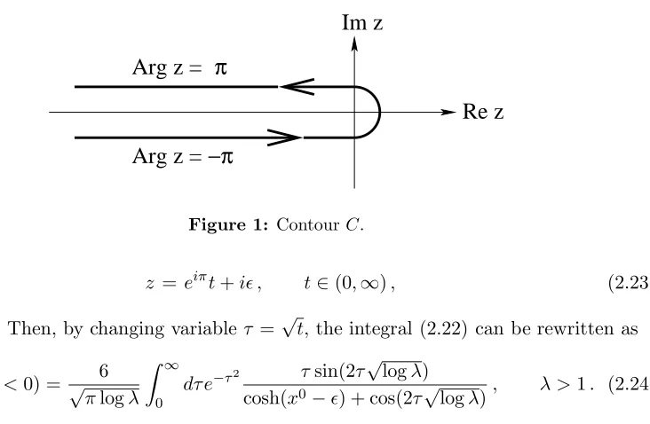
whereC is the path drawn in figure 1.

Thus, the integral oversin (2.18) can be explicitely performed,

Z γ+i∞

γ−i∞

ds

µ

4zlogλ t2

¶s

=iπ δhlogt−log³2pz logλ´i. (2.21)

In turn, integration of theδ-function leads to the expression

T(logλ, x0 <0) = 3

i√πlogλ

Z

C

dz e

z

1 +e2√zlogλ−x0 . (2.22)

It is easily realized that the contribution to the integral (2.22) given by the semicircle around the origin vanishes. The lower and upper branches of the pathCare parametrized, according to the notation of figure 1, as

z =e−iπt₋i² , t_∈(_∞,0),

3_{Another possibility would be that the odd derivatives of eq. (2.16) are discontinuous at the origin. This}

JHEP03(2005)079

Arg z =

Arg z =

Re z

Im z

[image:11.595.142.508.77.316.2]

−π

π

Figure 1: ContourC.

z =eiπt+i² , t_∈(0,_∞), (2.23)

respectively. Then, by changing variable τ =√t, the integral (2.22) can be rewritten as

T(logλ, x0<0) = √ 6 πlogλ

Z _∞

0

dτ e−τ2 τsin(2τ √

logλ)

cosh(x0_{−²) + cos(2τ}√_logλ), λ >1. (2.24)

Note that the hyperbolic cosine in (2.24) is always greater than one (x0 ≤0 and ² > 0), preventing any singularity in the integrand. Analogously, if we consider the case x0 > 0 in (2.14), we obtain forT(logλ, x0_{>0) an expression similar to (2.24) withx}0_{−²replaced} byx0+². Therefore, in any case no singularities arise and a representation for the tachyon field valid for any value ofx0 can be conveniently written as

T(logλ, x0) = √ 6 πlogλ

Z _∞

0

dτ e−τ2 τsin(2τ √

logλ)

e²_cosh(x0_{) + cos(2τ}√_logλ), λ >1. (2.25)

Eq. (2.25) provides the required analytical continuation of (2.11) to positive values of logλ. The regulator ² is immaterial for any point x0 6= 0 but it is crucial to prescribe the behavior at the origin. It guarantees that T(logλ, x0) _∈ C∞ in a neighbour of the origin and that all the odd derivatives of (2.25) vanish at x0 _{= 0. To understand the} mechanism, we can integrate by parts eq. (2.25) keeping²6= 0. After integration by parts, the singularities of the denominator that would appear atx0= 0 in the²_→0 limit become logarithmic (integrable) singularities. Then the regulator ²can be removed, obtaining

T(logλ, x0) = √ 3 πlogλ

Z _∞

0 dτ d

dτ

³

τ e−τ2´log[coshx0+ cos(2plogλτ)]. (2.26)

Iterating the procedure, any derivative of T can be written in a manifestly regular way. Note that, since ² can be eventually removed, it works as a prescription to define the integral (2.26) with all its derivatives. For example, the formula for the even derivatives of

T reads

d2nT(logλ, x0)

d(x0₎2n =

3(−1)n 22n√_π(logλ)n+1

Z _∞

0 dτ d

2n+1

dτ2n+1

³

τ e−τ2´log[coshx0+ cos(2plogλτ)].

[image:12.595.125.468.79.317.2]

JHEP03(2005)079

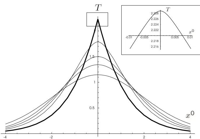
Figure 2: Different profiles of the solution T(logλ, x0_{). The bold profile refers to λ = λ}

c, the

remaining ones toλ1c/3,1, λc−1/3, λ−c1. As seen in the box, the behavior of the solution withλ=λc

is smooth at the origin.

The solutions (2.26) have the form of bounces, for any value ofλ. In figure 2 are drawn some profiles of the solutionT for different values ofλ. The bold profile refers to the physically relevant valueλ=λc, the remaining ones correspond toλ1c/3,1, λ−c1/3, λ−c1. Note the

man-ifest continuity inλexhibited in figure 2 passing form positive to negative values of logλ. To check the level of accuracy of the approximate solution (2.26) we must study the action of operators of the formq∂2

0 on it. At first sight, this is a non trivial problem, as the

x0-dependence in (2.26) is not through eigenfunctions of ∂₀2. Fortunately, eq. (2.26) still satisfies the diffusion equation (2.13), as can be checked by direct inspection. Therefore, the action of the operator q∂02 on T(logλ, x0) can be simply represented as a translation of logλ

q∂20_{T(logλ, x}0_{) =e}logq ∂20_{T(logλ, x}0_{) =e}−logq ∂

∂logλ_{T(logλ, x}0_{) =T(logλ}−_{logq, x}0_).

(2.28) This remarkable property can only be used thanks to the fact that we have treated the quantity λ as a generic variable. In particular we shall have often to make use of the following operator

λa∂02_{T(logλ, x}0_{) =}

∞ X

n=0

an(logλ) n

n!

∂2n

∂x02nT(logλ, x 0₎

=

∞ X

n=0

(₋a)n(logλ)

n

n!

∂n

∂(logλ)nT(logλ, x 0₎

= T((1₋a) logλ, x0). (2.29)

JHEP03(2005)079

A quantitative estimate of the accuracy of (2.26) can be obtained by calculating the

L2 norm of the left hand side (LHS(logλ, x0)) of eq. (2.6) evaluated on the approximate solution (2.26). If the solution of the equation was exact the value of this norm would be zero. Let us consider the physically relevant caseλ=λc. In this case theL2 norm ofLHS gives _||LHS_||2 = 4.636 _·10−8.

This value should be compared with a typical scale of the problem, for instance with theL2 norm of T, which is ||T||2 = 2.019. This shows the impressive level of accuracy of the solution (2.26) 4

µ

||LHS||2 ||T_||2

¶

λ=λc

∼2.3 _·10−8. (2.30)

3. Energy-momentum tensor

The tachyon field t(x0) appearing in the original form of the level truncated CSFT (1.1) is obtained by the field redefinition (2.5) applied to (2.26) with λ=λc. Using (2.29), one

hast(x0) =λc−5/3T(4₃logλc, x0), namely

t(x0) = 9λ

−5/3 c

4√πlogλc

Z _∞

0 d dτ

³

τ e−τ2´log[coshx0+ cos(4τplogλc/3)]. (3.1)

Eq. (3.1) is the analytic solution of our problem. It has the extremely good degree of accuracy (2.30) and it does not depend on any free parameter. In principle, one could try to improve the solution by introducing some external parameter in (3.1), but we have checked that this does not improve its accuracy.

Since we have at hand an action for the tachyon field, the energy-momentum tensor can be calculated as usual, by first including a metric tensorgµν in the action (1.1), varying

the action S with respect togµν and setting afterwards the metric to be flat,gµν =ηµν.

It is also possible to add a constant term₋α to the action (1.1). This is the only free constant we have and its choice can be dictated by physical considerations. In this way the tachyon potential reads

V[t] =−1

2t 2₊ λc

3 t

3_{+α . (3.2)}

Thus, we consider the action

S= 1

g2 o

Z

d26x√₋g

µ

1 2t

2

−1₂gµν∂µt ∂νt−

1 3λct˜

3 −α

¶

, (3.3)

where ˜t=λ

1 3¤

c t. The stress tensor then reads

Tαβ =−

2

√ −g

δS

δgαβ . (3.4)

4_{Another possibile check of the approximation would be to write eq. (2.6) as LHS = RHS, where}

LHS= (∂02−1)T, and to consider the quantity||LHS−RHS||2/||LHS||2. The order of magnitude of this

JHEP03(2005)079

In varying (3.3) with respect to the metric tensor, one has to consider the covariant form of the D’Alembertian operator

¤= √1 −g∂µ

√

−ggµν∂ν. (3.5)

The variation of the operator λ

1 3¤

c with respect to the metric can be performed by using

the following identity

δλ

1 3¤

c δgαβ =

1 3logλc

Z 1

0

ds λ13s¤

c

δ¤ δgαβ λ

1 3(1−s)¤

c . (3.6)

An alternative way to get the variation of the infinitely many derivatives operator λ

1 3¤

c

would be through a power series [15, 16] representation of the type (2.4). However, the remarkable property (2.29) of our solution is particularly well suited to deal with operators

of the type λ

1 3s¤

c . In fact, their action on T(logλc, x0) consists in a trivial translation

logλc → (1 + 1₃s) logλc. This will permit to write the energy momentum tensor in a

simple and closed form. Most importantly, it will be written as a bilinear in the fields

T(logλc, x0) containing only finite derivatives. Substituting infinite derivative operators

on the field T(x0_,logλ

c) with the field itself, but with the parameter λc traslated, allows

to write the energy momentum tensor in a form analogous to that of an ordinary (finite derivatives) field theory.

Taking the equation of motion (1.3) and eqs. (2.5), (2.29), (3.3)-(3.6) into account, after some integrations by parts we get the following expression for the energy-momentum tensor

Tαβ = λ−c10/3

(

δα0δβ0

µ

∂0T

µ

4

3logλc, x 0

¶¶2 +

+gαβ

·

1 2

µ

∂0T

µ

4

3logλc, x 0 ¶¶2 +1 2 µ T µ 4

3logλc, x 0

¶¶2 −

−1₃T

µ

5

3logλc, x 0

¶

(1₋∂₀2)T(logλc, x0)−αλ10c /3

¸

−

−1

3logλc

Z 1

0 ds

·

gαβ(1−∂02)T

µ

4−s

3 logλc, x 0

¶

∂₀2T

µ

4 +s

3 logλc, x 0

¶

+

+gαβ(1−∂02)∂0T

µ

4₋s

3 logλc, x 0

¶

×

×∂0T

µ

4 +s

3 logλc, x 0

¶¸

+

+ 2δα0δβ0(1−∂20)∂0T

µ

4₋s

3 logλc, x 0

¶

∂0T

µ

4 +s

3 logλc, x 0

¶)

. (3.7)

From (3.7) the explicit form of the energy density_E(x0_{) =T}

00and the pressurep(x0) =T11 can be obtained

E(x0) = λ−_c10/3

(

1 2

µ

∂0T

µ

4

3logλc, x 0

¶¶2 −1₂

µ

T

µ

4

3logλc, x 0

JHEP03(2005)079

+1 3T

µ

5

3logλc, x 0

¶

(1−∂₀2)T(logλc, x0) +αλ10c /3−

−1

3logλc

Z 1

0 ds

·

(1−∂₀2)T

µ

4−s

3 logλc, x 0

¶

∂₀2T

µ

4 +s

3 logλc, x 0

¶

−

−(1₋∂₀2)∂0T

µ

4−s

3 logλc, x 0

¶

×

×∂0T

µ

4 +s

3 logλc, x 0

¶¸)

, (3.8)

p(x0) = λ−_c10/3

(

1 2

µ

∂0T

µ

4

3logλc, x 0 ¶¶2 +1 2 µ T µ 4

3logλc, x 0

¶¶2 −

−1₃T

µ

5

3logλc, x 0

¶

(1₋∂₀2)T(logλc, x0)−αλ10c /3−

−1₃logλc

Z 1

0 ds

·

(1₋∂₀2)T

µ

4₋s

3 logλc, x 0

¶

∂₀2T

µ

4 +s

3 logλc, x 0

¶

+

+ (1₋∂₀2)∂0T

µ

4₋s

3 logλc, x 0

¶

×

×∂0T

µ

4 +s

3 logλc, x 0

¶¸)

. (3.9)

Even if from (3.8) the energy density seems to depend strongly on time, its plot will show that E(x0) is actually a constant. The energy density is conserved and is always identical to the chosen height of the maximum of the potential,E=α. The pressurep(x0) is an even function of x0_{, it has the shape of a bounce in time asymptotically reaching} the value ₋α. Thus, increasing the value of α in (3.2), the energy grows and the pressure lowers of the same amount.

The choice of α can strongly influence the physical picture described by the solu-tion (3.1). However, there are some features that are independent on this choice, namely the qualitative description of the tachyon motion and the asymptotic equation of state, which is alwaysp_{∼ −E} at x0 _{→ ±∞.}

Consider the time evolution of the solution, eq. (1.3) (or (2.6)) only admits even solutions and therefore the asymptotical states at x0 _{→ ±∞} must coincide. The motion is shown in figure 3. At x0 _{=−∞ the tachyon stays on the maximum A of the potential} V[t] (unstable vacuum). Since it has no kinetic energy, its energy density - that will be conserved during all its time evolution - is just V[0] = α. The pressure is negative (p=−α), forcing the tachyon to roll towards the minimum. As time evolves, the tachyon rolls and at x0_M = −0.144576 reaches the minimum M of the potential taking the value

t(x0

M) = 1/λc. Here the kinetic energy is maximal. Since E is conserved and the system

is classical, the tachyon cannot stop its motion and proceeds to an inversion point. This happens at x0 = 0, that corresponds to B in figure 3. Note that the value of the potential at the inversion pointBis lower than the value taken inA, still the energy being conserved. This is because the interaction felt by the tachyon is not described by V[t], as the cubic term in the interaction is “dressed” by the kinematical factor λ−∂20/3

[image:16.595.169.428.80.254.2]

JHEP03(2005)079

Figure 3: The tachyon potentialV[t]. The bold part ofV[t] refers to the motion A_→M_→B_→

M→A of the classical solutiont(x0_).

Figure 4: Energy density and pressure. The value of α = 0.056 is the minimum required to guarantee the DEC for any value ofx0_.

“dressing” is most significative when the acceleration is maximal, that is precisely at the inversion point B. This is the reason why the tachyon does not reach the point C in figure 3. For x0 _{> 0 the tachyon inverts its motion, passing again through the minimum} and asymptotically reaching the unstable maximumAatx0→+∞, where againp∼ −E =

−α. As already mentioned, different choices of α =_E simply raise or lower the profile of the pressure, that maintains the shape of a bounce. However, different values of α can describe different physical scenarios. Among all the possible choices, at least three deserve consideration.

We can fixα in such a way the Dominant Energy Condition (DEC)_{E ≥ |}p(x0_{)| holds} for any value of x0. This can be realized by choosing α ≥ 0.056. In the limiting case

[image:16.595.161.437.309.470.2]

JHEP03(2005)079

Other interesting choices can be obtained by fixing the physical properties of the matter distribution at the minimum M of the potential. One could require that the tachyon describes dust when reaches M. Thus, by imposing p(x0

M) = 0, one gets α= 0.103. With

this choice the DEC obvioulsy holds and the tachyon matter has the interesting equation of state p(x0) =w_E, with wthat smoothly interpolates between₋1 and 0 while the tachyon moves from the maximum to the minimum of its potential. Precisely as in the tachyon matter considered by Sen. The motion however continues passed the minimum of the potential and the pressure becomes positive. This form of tachyon matter is thus different to the one described in [18, 8, 19].

Another intersting scenario is realized by requiring that the DEC, E ≥ |p(x0)|, holds in x0 _{∈ (−∞,−x}0

M), i.e. during the rolling A → M from the unstable maximum to the

stable minimum of the potential. This is obtained by requiring that _E = _|p(x0

M)|, which

gives α = 0.051. Remarkably, the choice α = 0.051 reproduces the brane tension (that in these units is 1/(2π2_{)) within the 99% of accuracy. This might be an indication that the} solution we found might be the exact solution of the tachyon equation obtained by keeping into account also higher level fields. The equation we studied is certainly approximated, we wonder if the solution might be exact. In fact, since α just gives the height of the maximum of the potential, a natural choice for it would be the one that sets to zero the minimum of the potential. In this case, when coupled to gravity, the potential would not produce a cosmological constant term when the tachyon is at the minimum. At the (0,0) level truncation we are considering, such a constant is 1/(6λ2_c) (which is the 68% of the brane tension). When all the higher level fields are taken into account, the depth of the “effective” potential increases and the constant that sets to zero the minimum of the potential should reproduce theD-brane tension 1/(2π2). Thus, the DEC request naturally selects the correct depth of the potential when all levels are included.

4. Conclusions

In this paper we have shown that Cubic String Field Theory (CSFT) at the lowest order in the level truncation scheme has a classical rolling tachyon solution. This form of tachyon matter could have cosmological consequences. Having proven its existence directly from cubic string field theory, at least at this level of approximation, seems to provide a solid theoretical basis to tachyon driven cosmology.

Some interesting questions are raised by the CSFT rolling tachyon solution.

JHEP03(2005)079

• It would be interesting to consider the coupling of the decaying D-brane, described

by the rolling solution, to closed strings and study the emission of closed string from it. It would in particular be interesting to see if this would cause damped oscillations around the minimum or it might lead to a friction term that would just stop the rolling tachyon at the stable minimum of the potential.

• In order to provide a possible cosmological model it would be inconsistent not to take into account effects of gravity during the decaying process. The coupling of the cubic string field theory action to a Friedman-Robertson-Walker type metric is a formidable task because of the D’Alambertian operators in curved space that would appear in the action. If one could still assume the validity of the diffusion equation (2.13), this task could be, however, extremely simplifyed. This might provide an alternative to the Born-Infeld type effective action that has been so extensively used in the study of tachyon driven cosmology [3, 23, 25, 4, 26]. Cubic string field theory certainly provides a tachyon effective action that correctly describes tachyon physics [27, 28] and it is derived from first principles. In any case it should be at least possible to study the gravitational effects generated by the energy-momentum tensor of the rolling tachyon solution we have computed here, and see what kind of equations for the scale factor this will produce.

• The relationship between the rolling solution found here and the known solution in Boundary String Field Theory (BSFT) and vacuum string field theory [29, 30] is worth investigating [31]. The former is also related to the boundary conformal field theory approach, so that if a link could be established between the CSFT solution and the BSFT one, it should be possible to determine also the boundary state associated to the solution found here. This should shed some more light on the relations between the two approaches to string field theory [22]. It would be interesting to investigate also here the spatial inhomogeneous decay [6, 32].

• The solution found here does not contain free parameters, thus it should be compared with the half-S-brane case [6, 14] where the only parameter present can be set to 1 by a time translation. The full S-brane case [2, 33 – 35] contains instead a parameter whose sign provides a prescription for which side of the tachyon potential maximum the tachyon would roll. The CSFT solution we found does not present this possibility, the tachyon always rolls to the “right side”, i.e. to the side where the tachyon potential is bounded below.

Acknowledgments

G.G. is grateful to Gianluca Calcagni and in particular to Erasmo Coletti for useful dis-cussions.

References

JHEP03(2005)079

[2] A. Sen,Rolling tachyon,JHEP04 (2002) 048 [hep-th/0203211].

[3] G.W. Gibbons,Cosmological evolution of the rolling tachyon,Phys. Lett. B 537(2002) 1 [hep-th/0204008];Thoughts on tachyon cosmology,Class. Quant. Grav.20(2003) S321–S346 [hep-th/0301117].

[4] A. Sen,Remarks on tachyon driven cosmology,hep-th/0312153.

[5] E. Witten, On background independent open string field theory,Phys. Rev.D 46(1992) 5467 [hep-th/9208027];Some computations in background independent off-shell string theory,

Phys. Rev. D 47(1993) 3405 [hep-th/9210065];

S.L. Shatashvili,Comment on the background independent open string theory, Phys. Lett.B 311(1993) 83 [hep-th/9303143];On the problems with background independence in string theory,Alg. Anal. 6(1994) 215–226 [hep-th/9311177].

[6] F. Larsen, A. Naqvi and S. Terashima,Rolling tachyons and decaying branes, JHEP02

(2003) 039 [hep-th/0212248].

[7] J.A. Minahan,Rolling the tachyon in super BSFT,JHEP 07(2002) 030 [hep-th/0205098]. [8] S. Sugimoto and S. Terashima, Tachyon matter in boundary string field theory,JHEP 07

(2002) 025 [hep-th/0205085].

[9] E. Witten, Noncommutative geometry and string field theory,Nucl. Phys. B 268(1986) 253. [10] N. Moeller, A. Sen and B. Zwiebach,D-branes as tachyon lumps in string field theory,JHEP

08 (2000) 039 [hep-th/0005036].

[11] M. Fujita and H. Hata,Time dependent solution in cubic string field theory,JHEP 05(2003) 043 [hep-th/0304163].

[12] B. Chen, M. Li and F.-L. Lin,Gravitational radiation of rolling tachyon, JHEP11(2002) 050 [hep-th/0209222].

[13] T. Okuda and S. Sugimoto,Coupling of rolling tachyon to closed strings,Nucl. Phys.B 647

(2002) 101 [hep-th/0208196].

[14] N. Lambert, H. Liu and J. Maldacena,Closed strings from decaying D-branes,

hep-th/0303139.

[15] N. Moeller and B. Zwiebach,Dynamics with infinitely many time derivatives and rolling tachyons,JHEP10 (2002) 034 [hep-th/0207107].

[16] H.-t. Yang,Stress tensors in p-adic string theory and truncated OSFT,JHEP11 (2002) 007 [hep-th/0209197].

[17] T.G. Erler,Level truncation and rolling the tachyon in the lightcone basis for open string field theory,hep-th/0409179.

[18] A. Sen,Tachyon matter,JHEP 07(2002) 065 [hep-th/0203265];Field theory of tachyon matter, Mod. Phys. Lett.A 17(2002) 1797 [hep-th/0204143].

[19] A. Buchel, P. Langfelder and J. Walcher,Does the tachyon matter?,Ann. Phys. (NY)302

(2002) 78 [hep-th/0207235].

[20] A.A. Gerasimov and S.L. Shatashvili,On exact tachyon potential in open string field theory,

JHEP03(2005)079

[21] D. Kutasov, M. Marino and G.W. Moore,Some exact results on tachyon condensation in string field theory,JHEP 10(2000) 045 [hep-th/0009148].

[22] E. Coletti, V. Forini, G. Grignani, G. Nardelli and M. Orselli,Exact potential and scattering amplitudes from the tachyon non-linear beta-function,JHEP 03(2004) 030

[hep-th/0402167].

[23] L. Kofman and A. Linde,Problems with tachyon inflation, JHEP07(2002) 004 [hep-th/0205121].

[24] J.A. Minahan and B. Zwiebach,Field theory models for tachyon and gauge field string dynamics,JHEP 09(2000) 029 [hep-th/0008231];Effective tachyon dynamics in superstring theory,JHEP 03(2001) 038 [hep-th/0009246].

[25] A.V. Frolov, L. Kofman and A.A. Starobinsky,Prospects and problems of tachyon matter cosmology,Phys. Lett.B 545(2002) 8 [hep-th/0204187].

[26] M.R. Garousi, M. Sami and S. Tsujikawa,Inflation and dark energy arising from rolling massive scalar field on the D-brane,Phys. Rev. D 70(2004) 043536 [hep-th/0402075]. [27] W. Taylor,A perturbative analysis of tachyon condensation, JHEP03(2003) 029

[hep-th/0208149].

[28] W. Taylor and B. Zwiebach,D-branes, tachyons and string field theory,hep-th/0311017. [29] M. Fujita and H. Hata,Rolling tachyon solution in vacuum string field theory, Phys. Rev. D

70 (2004) 086010 [hep-th/0403031].

[30] L. Bonora, C. Maccaferri, R.J. Scherer Santos and D.D. Tolla,Exact time-localized solutions in vacuum string field theory,hep-th/0409063.

[31] V. Forini, G. Grignani and G. Nardelli, in preparation.

[32] A. Fotopoulos and A.A. Tseytlin,On open superstring partition function in inhomogeneous rolling tachyon background,JHEP 12(2003) 025 [hep-th/0310253].

[33] M. Gutperle and A. Strominger,Spacelike branes, JHEP04(2002) 018 [hep-th/0202210]. [34] A. Strominger,Open string creation by S-branes,hep-th/0209090.