City, University of London Institutional Repository
Citation
:
Häusler, W., De Martino, A., Ghosh, T. K. and Egger, R. (2008).
Tomonaga-Luttinger liquid parameters of magnetic waveguides in graphene. Physical Review B (PRB),
78, doi: 10.1103/PhysRevB.78.165402
This is the unspecified version of the paper.
This version of the publication may differ from the final published
version.
Permanent repository link:
http://openaccess.city.ac.uk/1660/
Link to published version
:
http://dx.doi.org/10.1103/PhysRevB.78.165402
Copyright and reuse:
City Research Online aims to make research
outputs of City, University of London available to a wider audience.
Copyright and Moral Rights remain with the author(s) and/or copyright
holders. URLs from City Research Online may be freely distributed and
linked to.
City Research Online:
http://openaccess.city.ac.uk/
publications@city.ac.uk
arXiv:0807.2606v2 [cond-mat.mes-hall] 5 Oct 2008
Tomonaga-Luttinger liquid parameters of magnetic waveguides in graphene
W. H¨ausler,1,2 A. De Martino,1,3 T.K. Ghosh,1,4 and R. Egger1
1Institut f¨ur Theoretische Physik, Heinrich-Heine-Universit¨at, D-40225 D¨usseldorf, Germany 2
Physikalisches Institut, Albert-Ludwigs-Universit¨at, D-79104 Freiburg, Germany
3Institut f¨ur Theoretische Physik, Universit¨at zu K¨oln, Z¨ulpicher Str. 77, D-50937 K¨oln, Germany 4Department of Physics, Indian Institute of Technology-Kanpur, Kanpur 208016, India
(Dated: October 6, 2008)
Electronic waveguides in graphene formed by counterpropagating snake states in suitable inho-mogeneous magnetic fields are shown to constitute a realization of a Tomonaga-Luttinger liquid. Due to the spatial separation of the right- and left-moving snake states, this non-Fermi liquid state induced by electron-electron interactions is essentially unaffected by disorder. We calculate the in-teraction parameters accounting for the absence of Galilei invariance in this system, and thereby demonstrate that non-Fermi liquid effects are significant and tunable in realistic geometries.
PACS numbers: 71.10.Pm, 73.21.-b, 73.63.-b
I. INTRODUCTION
One-dimensional (1D) electron systems can nowadays be studied in different material systems, e.g. by deposit-ing negatively charged metallic gate electrodes on top of a 2D electron gas (2DEG) in semiconducting heterostruc-tures, thereby depleting the 2DEG to form the de-sired structure,1 or in single-wall nanotubes (SWNTs).2
Such 1D quantum wires have been argued to realize the non-Fermi liquid behavior of a Tomonaga-Luttinger liq-uid (TLL),3,4,5,6,7 arising as a consequence of
electron-electron (e-e) interactions. Experimental signatures of TLL behavior include non-universal power laws in cer-tain transport properties related to the tunneling density of states, but many other observables also may reflect the non-Fermi liquid properties of a TLL. Experimental observations in semiconductor quantum wires8 were
ex-plained by TLL parameters of the order of gc ≈0.4 to
0.5, while the corresponding parameter in SWNTs9 was
reported as gc+ ≈ 0.16 to 0.3. Both values are
signifi-cantly smaller than the respective noninteracting value,
g= 1.
Very recently, graphene monolayers10,11 have become
available as a new realization of a 2DEG, albeit with properties strikingly different from their semiconducting counterparts. The kinetic energy of graphene close to one of the Dirac (K, K′) points is described by a two-component chiral Dirac-Weyl Hamiltonian12,13
H=vFτ·(p−A) (1) of massless relativistic particles moving at graphene’s Fermi velocity vF ≈ 106 m/sec, instead of the usual
Schr¨odinger Hamiltonian p2/2m∗ (with effective mass
m∗). In Eq. (1),τ denotes the vector of Pauli matrices in sublattice (“pseudo-spin”) space, while the physical spin as well as the valley (K−K′) degrees of freedom are left implicit. Furthermore, we have allowed for a static in-homogeneous orbital magnetic field perpendicular to the graphene plane (the field components in the plane do not affect orbital motion), B=B(x, y)ˆez, which is
incorpo-rated by minimal (Peierls) coupling in terms of the
cor-responding vector potential A(x, y). This gives rise to interesting magnetic barrier and magnetic confinement effects.14,15,16,17
It is well known, both theoretically18 and
experimentally,19 that a magnetic-field gradient can
give rise to unidirectional 1D snake states. Such orbits were recently studied theoretically in graphene20,21,22
and in SWNTs.23 Snake states carry current along the
lines where the magnetic field changes sign, and hence is zero. On a classical level, they can be understood as half-orbits of different circulation sense (for B > 0 andB <0), patched together to form a unidirectionally propagating orbit.24 Pairs of snake states running
antiparallel to each other are referred to as double snake states.25 In many regards, double snake states
correspond to the standard left- and right-movers in 1D quantum wires. For example, they should exhibit quantized conductance in multiples of 4e2/h (including
spin and valley degeneracies). Since the snake states are spatially separated, this quantization should be robust: shallow impurities are not expected to cause scattering between snake modes of opposite directionality.
In this work, we address consequences of the long-ranged but ultimately screened e-e interactions within and between the counterpropagating snake orbits in graphene magnetic waveguides. For a wide class of exper-imentally relevant field profiles, we show that a TLL state with broken Galilei invariance and extremely weak dis-order sensitivity can be realized. On a general level, the importance of e-e interactions for the correct interpreta-tion of experimental data in graphene has recently been stressed.26 Theories describing e-e interaction effects on
the transport properties of electrons in graphene have been proposed for strong homogeneous magnetic fields27
and for zero magnetic field.28 A recent debate has
dis-cussed the question whether interacting electrons in un-doped graphene form a Fermi liquid or not.29,30
Interac-tions are also predicted to yield a TLL state in special graphene nanoribbons with armchair edges.31
state,32,33 where the spin and valley degrees of freedom
give rise to the four channels. There is one charged (c+) channel, where the long-ranged e-e interactions play a crucial role, while the three neutral channels are basi-cally insensitive to interactions. We will see that the situation in a graphene magnetic waveguide is similar, and the parameter g discussed below plays the role of the SWNT parameter gc+. Albeit the interaction does
not spoil conductance quantization in dc transport for adiabatically connected reservoirs,34 it nevertheless
de-stroys the Fermi-liquid character of the system. In fact, it leads to non-universal power laws in the tunneling density of states, and to peculiar ac transport and shot noise35 properties at low temperatures. These
phenom-ena are appropriately described by TLL theory.3,4,5,6,7 The respective power-law exponents can be directly in-ferred from Refs. 32,33 by simply replacinggc+with our
estimate forg, see Eq. (32) below.
After introducing the model and the magnetic field profiles in Sec. II A, the bandstructure is studied in Gaus-sian approximation in what follows in Sec. II B. The ana-lytical bandstructure results are validated by comparing to exact diagonalization results. The numerical diago-nalization is briefly discussed in the Appendix. The lin-earized bandstructure for a double-snake state waveguide leading to TLL behavior is then described in Sec. III A. The physics of a TLL is governed by a dimensionless in-teraction parameter g, for which general expressions in terms of certain velocities are derived in Sec. III B. These velocities are obtained from perturbative expressions for the ground-state energy, and yield the analytical results forggiven in Sec. IV. We conclude in Sec. V. In Secs. III and IV, to be specific, we focus on electron-like excita-tions by assuming a positive value of the Fermi energy
εF. Below, we often take units such that~=vF= 1.
II. MODEL AND BANDSTRUCTURE
A. Model
In this paper, we consider magnetic fields B =B(x), guiding particles homogeneously along the y-direction. This implies that the wavenumberk along this direction is conserved. Two-component eigenstates of the Dirac-Weyl Hamiltonian (1) can then be written as ψ(x, y)∼
eiky(φ
k(x), χk(x))T. The vector potential can be chosen
asA=A(x)ˆey, with the spinor components obeying
0 −i∂x−ik+ iA(x)
−i∂x+ ik−iA(x) 0
φk(x)
χk(x)
=εk
φk(x)
χk(x)
. (2)
Complex phases may be chosen such thatφk is real and
χk purely imaginary. After squaring, Eq. (2) can be cast
into a Schr¨odinger-like form for the upper Dirac
compo-nentφk,
−∂x2+ [k−A(x)]2−B(x)−ε2k
φk(x) = 0. (3)
A similar equation holds for the lower componentχk(x),
with the sign of the “pseudo-Zeeman” term∼Breversed. Unlessεk= 0, Eq. (2) implies
Z
dx|φk(x)|2=
Z
dx|χk(x)|2= 1/2. (4)
Note that in path-integral approaches to relativistic quantum mechanics, in order to guarantee convergence of the Wiener measure,36 often the square of the Dirac
Hamiltonian (1) is considered. Path-integral represen-tations, on the other hand, allow for systematic ap-proximations, and therefore Eq. (3) is a useful starting point for the Gaussian approximation, cf. Sec. II B, where the boundedness of the differential operator appearing in Eq. (3) is exploited for either sign of B(x), in the spirit of a saddle-point approximation. Our method dif-fers from WKB-type approaches recently put forward to describe the electronic properties of graphene.22,37 We
note in passing that massive Schr¨odinger particles obey a related equation as Eq. (3), with quadratic momenta multiplied by 1/(2m∗), in the same magnetic field pro-file; only the pseudo-Zeeman term must be removed and, of course, the energyε2
k must be replaced byεk, i.e. hole
and zero-energy states both disappear. As a consequence, most of our conclusions also apply (at least qualitatively) to magnetic waveguides based on traditional Schr¨odinger fermions.
We consider the class of magnetic field profiles given by
B(x) =νωB(√ωBx)ν−1−B0. (5)
In our gauge, we thus have
A(x) =ω
ν+1 2
B x
ν
−B0x . (6)
The indexν can describe rather different situations, but we are only interested inν being a natural number. For instance, for ν = 1, we recover the homogeneous mag-netic field case, giving rise to the standard relativistic Landau levels. For ν = 2, the profile (5) instead de-scribes a setup with one snake state propagating along they-direction, whileν = 3 (or, more generally, all odd
ν > 1) can give rise to a double snake state geometry, where the background magnetic field−B0allows for lines
withB= 0, andωBsets the inhomogeneity scale.
Equa-tion (3) manifests the electron-hole symmetryεk↔ −εk
of Eq. (2), with a zero-energy eigenstate (εk = 0 for all
k) appearing wheneverν is odd, but not for evenν.38
3
also analyzed step-like field profiles, such as the ones de-scribed in Ref. 21, with very similar results and conclu-sions. For ν = 3, counterpropagating snake states are centered aroundx=±dwithB(±d) = 0, leading to
d=
√ B0
√
3ωB
, (7)
such that 2d is the parallel distance between counter-propagating snake states. In this configuration, a TLL can be realized, and most of our analysis will deal with this case.
Below, we will ignore the Zeeman splitting due to the interaction of the true electronic spin with the magnetic field creating the waveguide. A simple estimate for a homogeneous magnetic field already shows that this ap-proximation is justified in graphene. The physical Zee-man splitting ∆Z = geµBB amounts to 0.116 meV for
B= 1 Tesla, takingge = 2 and the free electron massme
going into Bohr’s magnetonµB. This value can be
com-pared to the orbital splitting ∆orb between subsequent
levels — in the language of Eq. (3), this corresponds to a “pseudo-Zeeman splitting” —, with the result
∆Z
∆orb ≃
εF
mev2F
, (8)
predicting that even forεF= 1 eV, the Zeeman splitting
is 50 times smaller than the orbital splitting. In view of the smallness of the ratio (8), we will neglect Zeeman terms in what follows. In any case, their effects on the low-energy theory of interacting electrons in graphene waveguides are standard, and could be included along the lines of Refs. 4,5,6,7.
B. Gaussian approximation
Next we describe our analytical approach to the band-structure and the eigenfunctions. They allow for closed form expressions of the TLL parameterg in Sec. IV. At large |k|, when anharmonic contributions of the effec-tive potential appearing in Eq. (3) are suppressed, the Gaussian approximation becomes exact. To confirm the accuracy of the analytical results, we have carried out numerical diagonalizations of the matrix representing the Schr¨odinger-like Hamiltonian (3) in a complete basis set. This is briefly described in the Appendix.
It is instructive to first study one of the two coun-terpropagating snake modes individually. We therefore set B0 = 0 and ν = 2 in Eq. (5), i.e. B(ξ) = 2ωBξ
withωB>0, where we introduce dimensionless lengths,
ξ=√ωBx, and momenta,κ=k/√ωB. The Schr¨odinger
version of this model has been studied previously.18The
single snake state is now centered nearx= 0 with (posi-tively or nega(posi-tively charged) particles running in the neg-ativey-direction. The spectrum in this case is not sym-metric,εk 6=ε−k. We then need to discuss the effective
potential appearing in Eq. (3),
Vν=2(κ, ξ) = (ξ2−κ)2−2τzξ ,
which depends on the sublattice component τz = ±1
of the wavefunction. Obviously, for anyκ, Vν=2 is
in-variant under the combined operation τz → −τz and
ξ → −ξ, so that |φk(ξ)| = |χk(−ξ)| in Eq. (2). For
κ→ −∞, the minima ofVν=2 approachκ2 at ξ= 0, so
that|φk(ξ)|=|χk(ξ)| ∼e−
√
−κ/2ξ2
and εk→−∞ → −k.
This indicates that the velocity reaches, up to sublead-ing corrections, the negative of the Fermi velocity. This is precisely the snake state, with both components of the Dirac spinor localized near x = 0. In the other limit,κ→+∞, the minima ofVν=2 approach−2√κat
ξ=τz√κ. In that case, the two sublattice components
|φk(ξ)|=|χk(−ξ)| ∼e−
√κ[ξ −√κ]2
are spatially separated from one another and from the snake mode, provided the distance exceeds the widths of these distributions. This result suggests an interesting application as a “sublat-tice filter”, where the magnetic field leads to a spatial separation of particles located on different sublattices. However, for the otherK point, the sublattice states are exchanged, and in order to see such an effect, one would need to have a valley-polarized system (i.e. a single K
point). The corresponding energy in Gaussian approxi-mation isεk→+∞ →0. This result cannot be recovered using WKB-type approaches22,37 which are more suited
to describe higher excited states. Interestingly, the posi-tionsξ=±√κof these states remain protected against the pseudo-Zeeman field “inclination” from Eq. (3), con-trary to naive expectation and in contrast to the non-zero shift found in any of the excited states. Finally, also ex-cited energies can be estimated in this way. For example, the first excited level is expected atεk= 2ω3B/8k1/4.
In effect, we then arrive at a picture where snake (near
x= 0) and “bulk” modes (nearx=±ω−B3/4√k) will de-velop. We here distinguish “snake” and “bulk” modes by their respective group velocities. Fig. 1 clearly demon-strates how the eigenstates evolve from snake states (at
k→ −∞with∂kεk =−1) into bulk modes atk→+∞.
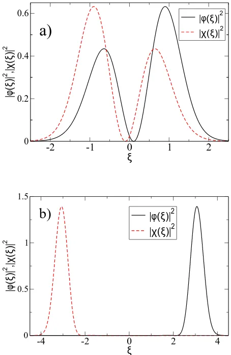
In Fig. 2 the corresponding metamorphosis is displayed of a (single) snake state at sufficiently negativekcentered aroundξ= 0, see Fig. 2(a), into a bulk state, residing in-creasingly far away fromξ= 0 with increasingk >0. For
κ= 8, cf. Fig. 2(b), the state is located nearξ= 2.83τz
as expected.
-2 0 2 4 6 8
k
0 1 2 3 4 5 6
ε k
FIG. 1: (Color online) Electron-like energy eigenvaluesεk ver-sus momentum k (both in units of √ωB), as obtained by numerical diagonalization of Eq. (3) for a magnetic field pro-file with ν = 2 and B0 = 0 in Eq. (5). The solid (black) curve denotes the lowest positive-energy eigenstate, and the dashed (red) and dash-dotted (blue) curves give the next two pairs of excited states. The dotted curve indicates the limit-ing snake-state dispersionεk =−kfor k <0, and the result in Gaussian approximation for the first excited energy band,
εk = 2ωB3/8k
1/4, for k > 0. Note that for the lowest state,
εk→+∞ approaches zero energy,
20,21 in agreement with the
Gaussian approximation.
is now symmetric, εk = ε−k. At k → ±∞, we thus
anticipate the coexistence of snake and bulk modes. In addition, an exact zero-energy eigenstate, εk = 0, must
now occur as a consequence of the index theorem.38The
potential entering Eq. (3) is
Vν=3(κ, ξ) = (ξ3−b0ξ−κ)2−τz(3ξ2−b0), (9)
where b0 =B0/ωB. This potential is invariant under a
simultaneous sign change of κ and ξ, transforming left-into right-movers and vice versa. Similar as for ν = 2, we can obtain energies in Gaussian approximation. The lowest energy, only forτz= +1, equals zero at large|k|.
This describes the zero-energy state, present for anykat oddν, cf. Sec. II A and the Appendix. The first excited (positive) energy is approximated as
εk=
√
6|ωBk|1/3+B0/[
√
6|ωBk|1/3]. (10)
This result is included to the numerically obtained spec-tra, see Fig. 3. The corresponding eigenstates are local-ized aroundξ= (|κ|1/3+b0/3|κ|1/3+τz/3|κ|)sgn(κ), i.e.
increasingly deep in the system’s bulk with increasing
|k|. Fig. 3 shows a typical spectrum obtained from nu-merical diagonalization. Depending on the slopes∂kεkat
large|k|, one type of bands goes likeεk ≃ ±vF|k|,
corre-sponding to the counterpropagating snake states centered aroundx=±d, see Eq. (7). Snake states move with the Fermi velocity of graphene at large|k|, irrespective of the magnetic field profile.20,21,39 The other bands in Fig. 3
exhibit smaller slopes at large |k|. The corresponding
-2 -1 0 1 2
ξ
[image:5.612.63.295.49.219.2] [image:5.612.326.553.50.399.2]0 0.2 0.4 0.6
|φ(ξ)|
2 ,|χ(ξ)|
2
|φ(ξ)|2 |χ(ξ)|2
a)
-4 -2 0 2 4
ξ 0
0.5 1 1.5
|φ(ξ)|
2 ,|χ(ξ)|
2
|φ(ξ)|2 |χ(ξ)|2
b)
FIG. 2: (Color online) Numerical diagonalization results for the probability densities of the spinor components |φκ(ξ)|2 (black solid curve) and |χκ(ξ)|2 (red dashed curve) of the lowest eigenstate to positive energy of Eq. (2) withν= 2 and
B0= 0. (a) is for momentumκ=−2, and (b) forκ= 8.
states are localized increasingly further away from the center of the wire at increasing|k|, and we thus call them again “bulk” modes. Due to their different slopes, bands of different types should cross, and Fig. 3 indeed reveals avoided intersections. Such avoided level crossings can be attributed to some residual hybridization between snake and bulk modes. They become successively less impor-tant as the bulk state’s center moves away from the snake state with increasing|k|.
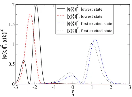
Fig. 4 validates the behavior of the two types of eigen-states for the double-snakeν= 3 situation withκ=−6. In view of Fig. 3, this value of |κ| is just beyond one of the (narrower) avoided crossings, so that the lowest positive-energy state, exhibiting a moderate slope, must be identified as a bulk state. This is indeed confirmed in Fig. 4, where the densities of both components of this state are seen. Gaussian approximation predicts its cen-ter to be atξ=−2.1 + 0.06τz, which is nicely confirmed
5
-4 -2 0 2 4
k 0
1 2 3 4 5 6 7
ε
kFIG. 3: (Color online) Same as Fig. 1 but forν= 3 andB0= 1.526ωB. Full curves (in different colors) give the numerical diagonalization results for the eigenenergies. When the Fermi level intersects only the lowest (black) curve, one has precisely one (spin- and valley-degenerate) left- and right-moving state in the waveguide. This leads to a TLL state. The dotted curve denotes εk = |k|, and the dashed curve gives the estimate (10) for the lowest dispersing energy band in the Gaussian approximation.
-3 -2 -1 0 1 2 3
ξ
[image:6.612.67.290.50.216.2] [image:6.612.63.292.374.543.2]0 0.5 1 1.5 2
|φ(ξ)|
2 ,|χ(ξ)|
2
|φ(ξ)|2, lowest state
|χ(ξ)|2, lowest state
|φ(ξ)|2, first excited state
|χ(ξ)|2, first excited state
FIG. 4: (Color online) Same as Fig. 2 but for a magnetic field (5) withν= 3 andB0= 1.525ωB. Shown are the two lowest positive-energy eigenstates withκ=−6.
classified as snake state. Indeed, as seen in Fig. 4, both pseudo-spin components of this state reside nearξ= 0.7, whereB(ξ) = 0. Note that, according to Eq. (22), densi-ties for oddν are mirror-symmetric under simultaneous sign reversal ofκandξ, so that theκ= +6 state is cen-tered atξ =−0.7. Finally, we note that all densities in Figs. 2 and 4 are well approximated by superpositions of suitable Gaussians, in accordance with our Gaussian description.
III. INTERACTION EFFECTS
A. Waveguide model
When considering a 1D graphene magnetic waveg-uide with counterpropagating snake states at low energy scales, see Sec. II B, the question arises whether inter-actingDirac fermions in such a waveguide belong to the TLL universality class.3,4,5,6,7 As always happens in 1D,
Landau quasiparticles will be destroyed by any non-zero e-e interaction strength,40but whether the resulting
non-Fermi liquid is a TLL remains to be shown. Indeed, this expectation is corroborated by the analogous situation in a quantum Hall bar,41,42 where, as a consequence of the
long-ranged Coulomb interaction between different edge states, a TLL with spatially separated left- and right-moving edge states emerges.43
We start with a discussion of the relevant single-particle bandstructure. For a magnetic waveguide with
ν = 3 andB0>0 in Eq. (5), the lowest positive-energy
subbandε(1)k =ε(1)−k has left- and right-going snake states nearx=±d, see Eq. (7), that essentially move at veloc-ity±vF. We assume that the Fermi level intersects these
states at±kF, and that all other states are energetically
sufficiently far away. This bandstructure was discussed in detail in Sec. II B, see Fig. 3. Using second quantization, the kinetic energy is then described by
H0=
X
k
ε(1)k c†kck, (11)
wherec†k (ck) creates (annihilates) a Dirac quasiparticle
with momentumk, and spin and valley indices are kept implicit. The electron field operator for waveguide length
Lalong they-direction is thus written as Ψ(x, y) = √1
L
X
k
eiky
φk(x)
χk(x)
ck . (12)
The crucial parameters characterizing the TLL are cer-tain velocities.5 In the noninteracting case, Dirac
parti-cles move at velocity21
vFhτyik= 2vFIm
Z dx φ∗
k(x)χk(x) =∂kεk≡vk ,
given by the slope of the energy dispersion, just as for Schr¨odinger particles. Assuming that εF is sufficiently
far away from both the band bottom of ε(1)k and from
the next-higher energy band, we linearizeε(1)k about the two Fermi pointsk=±kF, yielding velocities±vkF. This also separates right (k >0) from left (k <0) movers in Eq. (11), and implicitly defines the standard bandwidth cutoff around the Fermi level used in TLL theory.
B. Tomonaga-Luttinger liquid
potential44
W(x1,x2) =
e2
κ0
1
|x1−x2| −
1 p
(x1−x2)2+ 4D2
!
(13) between electrons at coordinatesx1= (x1, y1) andx2= (x2, y2). This form specifically accounts for screening
by metal gates positioned at some distance D from the waveguide. Its strength is governed by the dimensionless “fine structure constant”α=e2/[κ
0~vF], which basically
depends only on the dielectric constant κ0. For typical
substrate materials, one has values κ0 ≈1.4 to 4.7,
re-sulting in α ≈ 0.6 to 2.33,45,46 For graphene, both the
kinetic as well as the Coulomb energy scale (∼ √n for particle densityn) in the same way.46The resulting weak
tunability of the e-e interaction strength in graphene is in stark contrast to the situation in semiconductors, where
nallows to alter the relative strength of Coulomb inter-actions over orders of magnitude.
When constructing a low-energy theory for interact-ing Dirac fermions in the double snake state waveguide of Sec. III A, the resulting 1D e-e interaction processes can be classified as forward-scattering and backscatter-ing processes.3,4,5,6,7The spatial separation of the
unidi-rectional snake states here implies a strong suppression of e-e backscattering processes, where the relevant cou-plings are exponentially small in the parameterkFd≫1.
In the following, we discuss the regime
kFD≫kFd≫1, (14)
where backscattering processes are negligible. This situa-tion is reminiscent of the SWNT case,33where one,
how-ever, finds only an algebraic suppression of the backscat-tering couplings with increasing SWNT radius. We then only need to include forward-scattering processes, see also Ref. 33, and arrive at a four-channel TLL model. The three neutral sectors involve spin and valley degrees of freedom, and are decoupled from each other and from the charge sector (spin-charge separation). For not too strong interactions, as expected in graphene, the neutral sectors will remain basically unaffected by interactions, with their velocity parameters (almost) equal tovkF, see also Ref. 47. This implies that the TLL parameters for the three neutral sectors are just given by the noninter-acting value (g= 1). In the following, we then focus on the charge (c+) sector only.
The resulting TLL is most conveniently described by Abelian bosonization.4,5,6,7,33 For the c+ sector, the
re-sulting Hamiltonian is
Hc+= 1
2 Z
dy
vJ[∂yΘ(y)]2+vN[∂yΦ(y)]2 , (15)
with bosonic fields subject to the algebra [Φ(y), ∂yΘ(y)] = iδ(y − y′). Equation (15) reflects
the fact that density waves (in contrast to quasiparti-cles) are undamped in a TLL.40 With Eq. (15) and the
usual bosonized form of the Fermi operators,6 almost
any observable of physical interest can be determined exactly at low energies and long wavelengths, where the TLL model applies. In general, vJ < vN can deviate
from vkF as a result of the repulsive e-e interactions. Interaction physics is thus encoded invJ and vN. These
velocities determine the dimensionless TLL interaction parameterg≡gc+and the plasmon velocityv according
to4
g=pvJ/vN, v=√vJvN. (16)
In principle, both parameters are experimentally ac-cessible, e.g. through the tunneling density of states,9
momentum-resolved tunneling,8 or via plasmon
propa-gation times.48
The velocitiesvJandvNcan be extracted in an elegant
and exact manner from thermodynamic relations,5,49
vN=
π
4L ∂2E
0
∂k2 0
, vJ=
π
4L ∂2E
0
∂δ2 , (17)
provided the fully interacting ground-state energy den-sityE0/Lfor fixed left
−k(F−)
and rightkF(+)
Fermi
momenta is known, where δ = k(+)F −kF(−)/2 and
k0 =
kF(+)+kF(−)/2. The derivatives in Eq. (17) are evaluated atδ = 0 and k0 =kF, and the energyE0
in-cludes the spin and valley degrees of freedom. Clearly,vN
is proportional to the compressibility, and when Galilei invariance is realized,vJ =vkF is unchanged by interac-tions. However, as we shall see below, this symmetry is
notobeyed here due to the periodic superstructure im-posed by the snake orbit.
IV. TLL PARAMETER
Unfortunately, exact results forE0are known only for
a limited number of integrable models, such as the Hub-bard model50or the Sutherland model.51Even then, one still has to numerically solve coupled pairs of integral equations to accessE0, and hence the velocitiesvJ,N in
Eq. (17). In actual calculations ofvJandvNfor
noninte-grable models (which is the case here), one has to resort to approximations.44,52
A. Perturbation theory
We now use perturbation theory to obtainE0, and thus
the velocities (17), for relatively weak interactions. This approximation is almost exclusively used in the literature in order to obtain estimates for the TLL parameters of generic interacting 1D fermion systems. In that case, the ground-state energy can be split into three terms,
7
from which several contributions to the susceptibilities (17) follow. Accounting for spin and valley degeneracy, we have
∂2E kin
∂k2 0
=∂
2E kin
∂δ2 =
2L π (∂kε
(1) kF −∂kε
(1)
−kF) = 4L
π vkF , (19) as expected for noninteracting quasiparticles with veloc-ities±vkF.
From the Hartree interaction term, we then obtain
∂2E Hartree
∂k2 0
= L
π2
h
η(kF, kF) +η(kF,−kF) +R
i
, (20)
where, including again both spin and valley components, we define
η(k, k′) = η(k′, k) = 8 Z
dx
Z
dx′n
k(x)nk′(x′)
× αlnp1 + [2D/(x−x′)]2, (21)
with the particle density for wavevectorkat locationx,
nk(x) =|φk(x)|2+|χk(x)|2=n−k(−x). (22)
Note thatR
dx nk(x) = 1, see Eq. (4). Furthermore, we
have introduced the quantity
R =
Z kF
−kF
dk ∂kF[η(k, kF) +η(k,−kF)]
= 2
Z kF
0
dk ∂kF[η(k, kF) +η(k,−kF)]. (23)
The second equalities in Eqs. (22) and (23) are valid for all oddν >1. In Eq. (21), we have used that only long wavelengthsq→0 are important inEHartree. To see this,
consider the one-sided Fourier transform of Eq. (13),
W(q, x) = α
Z
dy eiqy 1
p
x2+y2 −
1 p
x2+y2+ 4D2
!
= αhK0(|qx|)−K0(|q|
p
4D2+x2)i, (24)
implying that W(q→ 0, x)≃αlnp
1 + [2D/x]2. With
these definitions, we obtain in a similar manner
∂2E Hartree
∂δ2 =
L π2
h
η(kF, kF)−η(kF,−kF) +R
i
. (25)
In view of Eqs. (16) to (25), only the magnitude of
η(kF,−kF) yields a nontrivial contribution to g at this
level of approximation. Within theg-ology terminology,3
we may identify this term withg2, measuring the strength
of forward scattering between particles of different direc-tionality (henceforth referred to as chirality). On the other hand, scattering between equal-chirality particles is described by g4, identified here as η(kF, kF).
How-ever, according to Eqs. (20) and (25), an additional term R is present, which effectively modifies g4. In
1D quantum wires with continuous (Galileian) transla-tional invariance, both nk(x) and η(k, k′) are
indepen-dent ofk, k′, and hence R= 0 and ∂2
δEHartree = 0. In
that case, the TLL parameter g depends only on the zero-momentum Fourier component of the interaction,
W(q ≃ 0) ≈ αln(D/d), where d is of the order of the wire width.
Similar (though slightly more involved) expressions can be found for the Fock contributions to Eq. (17), which are of the orderW(q≃2kF). Using Eq. (14), this amplitude
can be estimated as
W(2kF)≃α
r π
8kFde
−4kFd,
which is parametrically smaller than the Hartree am-plitude. Similar to backscattering contributions, Fock contributions can thus safely be neglected against the Hartree terms for the parameter regime (14).
B. TLL parameter estimate
In order to estimate the magnitude of the above terms, in particular ofη(kF,−kF), it is necessary to have some
handle on the unperturbed wavefunctions φk(x) and
χk(x), together with the resulting densities nk(x). We
approximate their density profiles as
nκ(ξ)≃
(12b0κ2)1/8
√ π e
−(12b0κ2)1/4[ξ+sgn(κ)√ωBd]2. (26)
Note that the true densities describing snake orbits, see Fig. 4, are somewhat more complicated, with a double-peak shape. However, the simplified single-Gaussian form in Eq. (26) captures the essential physics and al-lows for analytical progress.
Given Eq. (26), introducing the lengthscale
λ=
3
4B0ω
2 Bk2F
−1/8
, (27)
and using Eq. (21), we are now in a position to estimate
η(kF,−kF) ≃ 8αln(D/d),
η(kF, kF) ≃ 8αln
eC/2D/λ , (28) assuming D ≫ d ≫ λ, see Eq. (14). Here C = 0.577. . . is the Euler constant. We see that the ratio
η(kF,−kF)/η(kF, kF) approaches unity forD→ ∞as in
Galilei-invariant 1D wires, where in addition one also has
R= 0. In order to estimate R, we first observe that in Eq. (23), the η(k,−kF) term is suppressed by a factor
e−8(d/λ)2
as compared to η(k, kF). This factor becomes
small in the regime (14), and we can therefore approxi-mateR ≃2RkF
0 dk ∂kFη(k, kF),which can be calculated in closed form for the density profile (26),
R ≃ 8αh√2(c1+ 2c2) + 4(
√
2c1−1) ln(D/λ)
i
Employing the incomplete Euler Beta function, we find
c1=
1 3
4√2−
Z 1
0
dt √
1 +t t3/4
≃0.6496 (30)
and
c2=
Z 1
0
dt t
1/4
√
1 +tln
1 +t
1 +√t
≃ −0.07171. (31)
Remarkably, R decreases with increasing D/λ, changes sign atD≃9.02λ, and then continues to decrease loga-rithmically. Although asymptotically smaller by a factor 4(√2c1−1)≃0.326 than the leading contribution (28) to
g4, theR-term is important for quantitative estimates of
the TLL parameter. For example, whenR<0, standard expressions (withoutR) would overestimateg, pretend-ing too weak interaction effects. The usual expressions are based on Galilei invariance, which is broken in the present system due to the periodic superstructure im-posed on the 1D wire by the snake orbits. It is not ob-vious to us how standard estimates tog4, starting from
the microscopic interaction (13), would recover the R -contribution.
Combining Eqs. (16) to (29), we get the analytical es-timate for the TLL parameter,
g≃
g
0−ln(D/d)
g0+ ln(D/d)
1/2
, (32)
in the regimeD≫d≫λ, see Eq. (14), whereλis given in Eq. (27). Here, we have abbreviated
g0 =
π
2α+ √
2(c1+ 2c2) + 4(
√
2c1−1) ln
D λ
+ ln
eC/2D λ
. (33)
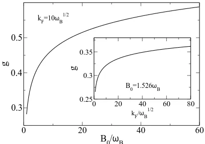
The TLL parameter (32) is depicted in Fig. 5, where
|∂kεkF|=vF and a “fine structure constant”α= 1 have been assumed. However, according to Eq. (33), changes in α may be compensated for via changes in λ, i.e. by modification ofkFor of the magnetic field parameters.
As shown in the inset of Fig. 5, values of aboutg≈0.3 are expected for the chosen value of B0, with no
pro-nounced variations when changingD/λ. Such weak sen-sitivity to kF found in graphene is in stark contrast
to semiconducting wires, whereg can vary significantly when changing the carrier density.44As discussed in the
Introduction, similar values forgas compared to the val-ues in Fig. 5 have been reported for other TLL systems such as quantum wires8 or SWNTs.9,32,33 On the other
hand, the main panel in Fig. 5 demonstrates thatg can be widely tuned in graphene wires by changing the snake-state separation 2din Eq. (7) via the magnetic field pa-rameters, in particular by sweeping the background field
B0.
0 20 40 60
B0/ωB
0.3 0.4 0.5
g
kF=10ωB1/2
0 20 40 60 80
kF/ωB1/2
0.25 0.3 0.35
g
[image:9.612.336.542.50.195.2]B0=1.526ωB
FIG. 5: TLL parameter g in Eq. (32) for α = 1 and D = 100/√ωB. Main panel: g as a function of B0/ωB for kF = 10√ωB. Inset: g vskF/√ωB for B0 = 1.526ωB. Note that the regimeλ ≪ dtranslates into kF ≫ √18
3ω 2 BB−
5/2 0 , which here implieskF/√ωB>1.
V. CONCLUSIONS
In this paper, we have analyzed the effects of electron-electron interactions on the electron-electronic properties of netic waveguides formed in suitable inhomogeneous mag-netic fields in graphene. When there are two parallel lines along which the magnetic field vanishes, a pair of counterpropagating snake states can be formed, which are ideal unidirectional (chiral) channels similar to the edge states in quantum Hall bars. We have studied the case of a smooth magnetic field profile across the wire, but similar results are expected also for other profiles, e.g. for piece-wise constant fields. Employing a combi-nation of analytical methods for the band structure and for the eigenfunctions (which were checked against ex-act diagonalization results) with a thermodynamical ap-proach, we have obtained a closed result for the non-universal TLL parameter, see Eq. (32) and Fig. 5. This parameter then determines the power-law exponents ap-pearing in many observables of interest, in particular in the energy-dependence of the tunneling density of states. Quite remarkably, we have uncovered that the snake or-bits impose a periodic superstructure that breaks Galilei invariance of the resulting wire, and modifies the com-monly used estimate for the TLL parameter g. The fi-nite R-term in Eq. (29) reflects this physics. We ex-pect this correction to affect also edge states in quantum Hall bars. Typical values for g found here are compa-rable to the values reported for semiconductor quantum wires and single-wall carbon nanotubes. We thus expect that non-Fermi liquid behavior should be sufficiently pro-nounced to be observable in systems based on inhomoge-neous magnetic fields.
9
of the homogeneous part of the magnetic profile. This is illustrated in the main panel of Fig. 5. Second, the unavoidable presence of disorder is not expected to affect the TLL behavior, since right- and left-moving electrons are spatially separated. This may allow, for the first time, to experimentally study the physics of an ultraclean TLL state.
While there are similarities to the physics of quantum Hall edge states, the TLL state discussed here is quite different from the chiral Luttinger liquid discussed in the context of the fractional quantum Hall effect.42 The g
parameter in the latter case is fixed by the bulk filling factor, while here it is non-universal and tunable. From a conceptual point of view, the quantum Hall situation is also more intricate because of the coupling of edge states to bulk states.42 Such complications are absent for the
TLL state discussed in this paper. To conclude, we hope that our work motivates experiments in this direction.
Acknowledgments
We thank T. Heinzel for discussions. WH would like to thank H. Grabert for continuous support. This work has been supported by the SFB -TR/12, by the ESF IN-STANS program, and by the A. v. Humboldt foundation.
NUMERICAL DIAGONALIZATION
In this Appendix, we provide some details on how the numerical diagonalization mentioned in Sec. II B has been implemented. From Eq. (6), we first observe that exact eigenfunctions φ(x) of Eq. (3) behave as
∼exph−x1+1+νν
i
forx→ ∞. For example, the exact zero-energy state to Eq. (9) is given as (e−ξ4
/4+b0ξ2/2+κξ,0)T up to a normalization factor.
However, it is clear that accurate eigenvalues ε2 k only
require to maximize the overlap between the
approxi-mated wavefunction andφ(x). For convenience, we thus use the complete and orthonormal oscillator basis
ϕn(ξ) =
1
π1/4√2nn!e
−ξ2/2
Hn(ξ),
where Hn are Hermite polynomials. Matrix elements
of the operator H2 in Eq. (3) in this basis read (b 0 =
B0/ωB)
ωB−1hϕn|H2|ϕn′i= (2n+ 1 +κ2)δnn′
+hϕn|ξ2ν−(1−b20)ξ2−2b0ξν+1|ϕn′i
−hϕn|2k(ξν−b0ξ)−τz(νξν−1−b0)|ϕn′i,
where we use that for integerγ and evenn+n′+γ (Γ denotes the Gamma function)
hϕn|ξγ|ϕn′i=
r
2n+n′n!n′!
π
[n/2]
X
m=0 [n′/2]
X
m′=0
−1
4
m+m′
× Γ(
1+n+n′+γ
2 −m−m′)
m!m′! (n−2m)! (n′−2m′)! ,
where hϕn|ξγ|ϕn′i = 0 otherwise. The symbol [n]
de-notes the largest integer smaller or equal to n. Upon carrying out standard diagonalization for 0≤n, n′≤30 basis functions, we obtain the energy dispersion εk in
Figs. 1 and 3 for ν = 2 and ν = 3, respectively. To numerical accuracy, all levels are found independent of
τz=±1, although the effective potentials in Eq. (3)
dif-fer considerably. Only the zero-energy level εk = 0 in
Fig. 3 (there is no zero-energy level in Fig. 1) belongs purely to the upper pseudo-spin componentτz= +1 for
the valley pointKchosen here. With the numerical diag-onalization, we also obtain the eigenfunctionsφk(x) and
χk(x) of the Dirac Hamiltonian (2). In Figs. 2 and 4, we
show the resulting density profiles forν = 2 and ν = 3, respectively. All figures nicely confirm the overall picture developed in Sec. II B.
1 For reviews, see e.g.Quantum transport in ultrasmall
de-vices, NATO Adv. Studies Institute Series B, Vol. 342, ed. by D.K. Ferry (Plenum, New York, 1995).
2 Carbon nanotubes: Synthesis, Structure, Properties, and
Applications, ed. by M.S. Dresselhaus, G. Dresselhaus, and Ph. Avouris, Springer Topics in Applied Physics, Vol. 80 (Springer, Berlin, 2001).
3 J. S´olyom, Adv. Phys.28, 201 (1979). 4 F.D.M. Haldane, J. Phys. C
14, 2585 (1981). 5 J. Voit, Rep. Prog. Phys.57, 977 (1994).
6 A.O. Gogolin, A.A. Nersesyan, and A.M. Tsvelik,
Bosonization and Strongly Correlated Systems (Cam-bridge University Press, 1998).
7 T. Giamarchi, Quantum Physics in One Dimension (Ox-ford University Press, 2003).
8 For very recent experimental reports on TLL behavior in
semiconductor quantum wires, see H. Steinberg, G. Barak, A. Yacoby, L.N. Pfeiffer, K.W. West, B.I. Halperin, and K. Le Hur, Nature Physics 4, 116 (2008), and references therein.
9 M. Bockrath, D.H. Cobden, J. Lu, A.G. Rinzler, R.E.
Smalley, L. Balents, and P.L. McEuen, Nature 397, 598 (1999); Z. Yao, H.W.Ch. Postma, L. Balents, and C. Dekker, ibid. 402, 273 (1999); B. Gao, A. Komnik, R. Egger, D.C. Glattli, and A. Bachtold, Phys. Rev. Lett.92, 216804 (2004).
10 K.S. Novoselov, A.K. Geim, S.V. Morozov, D. Jiang, Y.
201 (2005); C. Berger, Z. Song, X. Li, X. Wu, N. Brown, C. Naud, D. Mayou, T. Li, J. Hass, A.N. Marchenkov, E.H. Conrad, P.N. First, and W.A. de Heer, Science312, 1191 (2006); F. Molitor, J. G¨uttinger, C. Stampfer, D. Graf, T. Ihn, and K. Ensslin, Phys. Rev. B76, 245426 (2007). 11 For a review, see A.K. Geim and K.S. Novoselov, Nature
Materials6, 183 (2007).
12 We absorb the factore/cintoA andB.
13 G.W. Semenoff, Phys. Rev. Lett. 53, 2449 (1984); D.P.
DiVincenzo and E.J. Mele, Phys. Rev. B29, 1685 (1984). 14 F.M. Peeters and A. Matulis, Phys. Rev. B
48, 15166 (1993); N. Malkova, I. G´omez, and F. Dom´ınguez-Adame,
ibid.63, 035317 (2001); S.M. Badalyan and F.M. Peeters,
ibid.64, 155303 (2001); J.M. Pereira, Jr., F.M. Peeters, and P. Vasilopoulos,ibid.75, 125433 (2007).
15 S.J. Lee, S. Souma, G. Ihm, and K.J. Chang, Physics
Re-ports394, 1 (2004).
16 A. De Martino, L. Dell’Anna, and R. Egger, Phys. Rev.
Lett.98, 066802 (2007).
17 M. Ramezani Masir, P. Vasilopoulos, A. Matulis, and F.M.
Peeters, Phys. Rev. B77, 235443 (2008).
18 J.E. M¨uller, Phys. Rev. Lett.68, 385 (1992); J. Reijiniers
and F.M. Peeters, J. Phys.: Condens. Matter 12, 9771 (2000); J. Reijiniers, A. Matulis, K. Chang, F.M. Peeters, and P. Vasilopoulos, Europhys. Lett. 59, 749 (2002); H. Xu, T. Heinzel, M. Evaldsson, S. Ihnatsenka, and I.V. Zo-zoulenko, Phys. Rev. B75, 205301 (2007).
19 P.D. Ye, D. Weiss, R.R. Gerhardts, M. Seeger, K. von
Klitzing, K. Eberl, and H. Nickel, Phys. Rev. Lett. 74, 3013 (1995); D. Lawton, A. Nogaret, M.V. Makarenko, O.V. Kibis, S.J. Bending, and M. Henini, Physica E,13, 699 (2002); M. Hara, A. Endo, S. Katsumoto, and Y. Iye, Phys. Rev. B69, 153304 (2004); M. Cerchez, S. Hugger, T. Heinzel, and N. Schulz,ibid.75, 035341 (2007). 20 L. Oroszl´any, P. Rakyta, A. Korm´anyos, C.J. Lambert,
and J. Cserti, Phys. Rev. B77, 081403(R) (2008). 21 T.K. Ghosh, A. De Martino, W. H¨ausler, L. Dell’Anna,
and R. Egger, Phys. Rev. B77, 081404(R) (2008). 22 A. Korm´anyos, P. Rakyta, L. Oroszl´any, and J. Cserti,
arXiv:0805.2527.
23 H.-W. Lee and D.S. Novikov, Phys. Rev. B 68, 155402
(2003); N. Nemec and G. Cuniberti, ibid. 74, 165411 (2006).
24 In thermal equilibrium, unidirectional 1D states must
occur in pairs of counterpropagating snake (or edge) modes.20,21
25 A. Nogaret, S.J. Bending, and M. Henini, Phys. Rev. Lett.
84, 2231 (2000).
26 A. Bostwick, T. Ohta, T. Seyller, K. Horn, and E.
Roten-berg, Nature Physics3, 36 (2007).
27 M.O. Goerbig, R. Moessner, and B. Dou¸cot, Phys. Rev. B
74, 161407(R) (2006); K. Nomura and A.H. MacDonald, Phys. Rev. Lett.96, 256602 (2006); L. Sheng, D.N. Sheng, F.D.M. Haldane, and L. Balents,ibid.99, 196802 (2007); C.-H. Zhang and Y.N. Joglekar, Phys. Rev. B75, 245414 (2007).
28 T. Ando, J. Phys. Soc. Jpn. 75, 074716 (2006); V.V.
Cheianov and V.I. Fal’ko, Phys. Rev. Lett. 97, 226801
(2006); E.G. Mishchenko,ibid.98, 216801 (2007); Y. Bar-las, T. Pereg-Barnea, M. Polini, R. Asgari, and A.H. Mac-Donald,ibid.98, 236601 (2007); E. Mariani, L.I. Glazman, A. Kamenev, and F. von Oppen, Phys. Rev. B76, 165402 (2007).
29 J. Gonzalez, F. Guinea, and M.A.H. Vozmediano, Nucl.
Phys. B424, 595 (1994); Phys. Rev. B63, 134421 (2001); T. Stauber, F. Guinea, and M.A.H. Vozmediano,ibid.71, 041406(R) (2005); D.T. Son,ibid.75, 235423 (2007). 30 I.F. Herbut, Phys. Rev. Lett.
97, 146401 (2006); D.V. Khveshchenko, Phys. Rev. B74, 161402(R) (2006); S. Das Sarma, E.H. Hwang, W.-K. Tse, ibid.75, 121406 (2007); I.F. Herbut, V. Juricic, and O. Vafek, Phys. Rev. Lett.
100, 046403 (2008).
31 H.A. Fertig and L. Brey, Phys. Rev. Lett. 97, 116805
(2006); M. Zarea and N. Sandler,ibid.99, 256804 (2007). 32 R. Egger and A.O. Gogolin, Phys. Rev. Lett.
79, 5082 (1997); C. Kane, L. Balents, and M.P.A. Fisher, ibid.79, 5086 (1997).
33 R. Egger and A.O. Gogolin, Eur. Phys. J. B
3, 281 (1998). 34 I. Safi and H.J. Schulz, Phys. Rev. B52, R17040 (1995). 35 B. Trauzettel, R. Egger, and H. Grabert, Phys. Rev. Lett.
88, 116401 (2002); F. Dolcini, B. Trauzettel, I. Safi, and H. Grabert, Phys. Rev. B71, 165309 (2005).
36 L.C. Biedenharn, Phys. Rev. 126, 845 (1962); G.J.
Pa-padopoulos and J.T. Devreese, Phys. Rev. D 13, 2227 (1976); M.A. Kayed and A. Inomata, Phys. Rev. Lett.53, 107 (1984); T. Boudjedaa, L. Chetouani, L. Guechi, and T.F. Hammann, Physica Scripta46, 289 (1992).
37 P. Carmier and D. Ullmo, arXiv:0801.4727.
38 Y. Aharonov and A. Casher, Phys. Rev. A19, 2461 (1979);
L. Erd¨os and V. Vougalter, Commun. Math. Phys. 225, 299 (2002).
39 S. Park and H.-S. Sim, Phys. Rev. B
77, 075433 (2008). 40 I.E. Dzyaloshinski˘ı and A.I. Larkin, Zh. ´Eksp. Teor. Phys.
65, 411 (1973) [Sov. Phys. JETP38, 202 (1974)]. 41 B.I. Halperin, Phys. Rev. B 25, 2185 (1982); A.H.
Mac-Donald, Phys. Rev. Lett.64, 220 (1990). 42 A.M. Chang, Rev. Mod. Phys.
75, 1449 (2003).
43 U. Z¨ulicke and A.H. MacDonald, Phys. Rev. B54, 16813
(1996).
44 W. H¨ausler, L. Kecke, and A.H. MacDonald, Phys. Rev. B
65, 085104 (2002).
45 J. Alicea and M.P.A. Fisher, Phys. Rev. B 74, 075422
(2006).
46 H.P. Dahal, Y.N. Joglekar, K.S. Bedell, and A.V. Balatsky,
Phys. Rev. B74, 233405 (2006).
47 C.E. Creffield, W. H¨ausler, and A.H. MacDonald,
Euro-phys. Lett.53, 221 (2001).
48 G. Ernst, N.B. Zhitenev, R.J. Haug, and K. von Klitzing,
Phys. Rev. Lett.79, 3748 (1997).
49 This also applies to multiband situations, cf. W. H¨ausler,
Phys. Rev. B70, 115313 (2004).
50 E. Lieb and F.Y. Wu, Phys. Rev. Lett.20, 1445 (1968). 51 N. Kawakami and S.-K. Yang, Phys. Rev. Lett.
67, 2493 (1991).