Miatto, F. M. and Giovannini, D. and Romero, J. and Franke-Arnold, S.
and Barnett, S. M. and Padgett, M. J. (2012) Bounds and optimisation of
orbital angular momentum bandwidths within parametric
down-conversion systems. European Physical Journal D: Atomic, Molecular,
Optical and Plasma Physics, 66 (7). -. ISSN 1434-6060 ,
http://dx.doi.org/10.1140/epjd/e2012-20736-x
This version is available at
https://strathprints.strath.ac.uk/41380/
Strathprints is designed to allow users to access the research output of the University of Strathclyde. Unless otherwise explicitly stated on the manuscript, Copyright © and Moral Rights for the papers on this site are retained by the individual authors and/or other copyright owners. Please check the manuscript for details of any other licences that may have been applied. You may not engage in further distribution of the material for any profitmaking activities or any commercial gain. You may freely distribute both the url (https://strathprints.strath.ac.uk/) and the content of this paper for research or private study, educational, or not-for-profit purposes without prior permission or charge.
Any correspondence concerning this service should be sent to the Strathprints administrator: [email protected]
The Strathprints institutional repository (https://strathprints.strath.ac.uk) is a digital archive of University of Strathclyde research outputs. It has been developed to disseminate open access research outputs, expose data about those outputs, and enable the
DOI:10.1140/epjd/e2012-20736-x
Regular Article
P
HYSICAL
J
OURNAL
D
Bounds and optimisation of orbital angular momentum
bandwidths within parametric down-conversion systems
F.M. Miatto1,a, D. Giovannini2, J. Romero2, S. Franke-Arnold2, S.M. Barnett1, and M.J. Padgett2
1
SUPA and Department of Physics, University of Strathclyde, G4 0NG Glasgow, UK 2
School of Physics and Astronomy, SUPA, University of Glasgow, G12 8QQ Glasgow, UK
Received 15 December 2011
Published online 10 July 2012 – cEDP Sciences, Societ`a Italiana di Fisica, Springer-Verlag 2012
Abstract. The measurement of high-dimensional entangled states of orbital angular momentum prepared by spontaneous parametric down-conversion can be considered in two separate stages: a generation stage and a detection stage. Given a certain number of generated modes, the number of measured modes is determined by the measurement apparatus. We derive a simple relationship between the generation and detection parameters and the number of measured entangled modes.
1 Introduction
Entangled states are a distinctive feature of quantum me-chanics. Their use can lead to important technological ad-vances in communication, security and, ultimately, com-puting [1]. Entanglement in a high-dimensional Hilbert space means a high effective number of entangled modes that can be used to achieve a high shared information [2]. It is therefore of great importance to choose the proper basis in which to detect entangled modes. The Schmidt basis is that which yields the maximum shared informa-tion [3]. For most entangled states, however, the elements of the Schmidt basis cannot readily be measured, perhaps because the size of the components in the detection appa-ratus do not match any possible detection mode [4].
It is well-known that light can carry orbital angu-lar momentum (OAM) and that this property is as-sociated with a helical phase front [5] (and papers reprinted therein). Optical modes carrying OAM include the Laguerre-Gaussian modes [6] and also the Bessel beams. Of central interest to us in this paper is the fact that photon pairs produced in spontaneous parametric down-conversion (SPDC) are naturally entangled in their OAM [7–9]. One clear manifestation of this entanglement is the existence of an EPR paradox for the OAM and its conjugate quantum variable, the azimuthal angle [10–12]. The OAM is conserved in the down-conversion process and hence for a Gaussian (ℓ= 0) pump, the OAM of the signal and idler fields are perfectly anticorrelated. There are also correlations on the radial direction (as quanti-fied, for the Laguerre-Gaussian modes, by a radial in-dex p) [13] but these will not concern us in this paper. Our central concern will be the number of entangled low-est order (p= 0) Laguerre-Gaussian modes generated in
a
e-mail:[email protected]
a down-conversion experiment. The typical setup that we consider is a type-I or type-II, degenerate SPDC setup. We work in the regime of undepleted pump and we ne-glect eventual anisotropies of the down-converted beams. We find that, for any given set of generation parame-ters (pump waistwp, wavelengthλ, crystal lengthL) the detection apparatus can be prepared in a way that max-imises the measured number of entangled modes and that two important parameters areγ, the ratio of the width of the pump beam to the width of the detection modes, and LR, the length of the crystal normalised to the Rayleigh range of the pump beam:
γs,i= wp ws,i
and LR= L zR
(1)
where the Rayleigh range is zR = πw2
p
λ . In this paper we assume that the signal and idler modes have the same width so thatws=wi andγs=γi=γ.
The precise calculation ofws,i depends upon the de-tails of the detection system. Our analysis can be applied if the back-projected detection mode size,wi,s, is approx-imatelyℓ-independent over the range of OAM of interest, and if the modes with p= 0 couple only weakly with the fundamental mode of the fibre that carries the signal to the coincidence counter.
Page 2 of6 Eur. Phys. J. D(2012) 66: 178
and to the characterisation of the detection parameters. We present both an analytical treatment and also a simple geometrical argument for our results.
The second section of the paper specifies the definitions of the various bandwidths which are used. The third sec-tion contains the analytical approach to calculate the pro-jection amplitudes. The fourth section contains the geo-metrical approach to calculate a simple formula that gives the measurement bandwidth. The fifth section contains the interpretation of the results and the conclusions.
2 Definition of bandwidths
For a distribution of probabilities, in our case for the OAM of the signal or idler photon in SPDC, we can define a number of statistical measures. For high-dimensional en-tanglement we require as many modes as possible to con-tribute to the state and, moreover, for these to concon-tribute strongly, that is to have a significant probability. A simple and convenient measure of this quantity is the Schmidt number [21,22]:
K({pi}) := 1
ip2i
, (2)
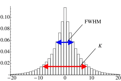
where the probabilities {pi} are, in our case, those for each of the OAM modes. The measure K gives the effec-tive number of contributing modes and hence the effeceffec-tive dimensionality of the system. In experiments, it is typical to quote the full-width at half maximum as the measure of the bandwidth (FWHM) so as to include only modes that are well above the noise floor. FWHM should not be con-fused withK. For simple, symmetrical and single-peaked probability distributions, the Schmidt number provides a convenient measure of the bandwidth. The precise rela-tionship between the Schmidt number and the FWHM depends upon the detailed shape of the distribution but typical of our systems is that theK exceeds the FWHM, see Figure 1. For a distribution like this we can define an effective range of modes contributing to the state ranging fromℓmax toℓmin=−ℓmax such thatK= 1 + 2|ℓmax|.
The generation bandwidth is the effective number of entangled modes generated in the SPDC process. As it does not depend on the detection apparatus, it is a func-tion only of the crystal length and of the size of the pump beam, combined into the quantity LR, defined in equa-tion (1). This bandwidth can be thought of as the dimen-sionality of the entanglement in OAM and can be calcu-lated through the Schmidt decomposition of the SPDC state [4]. More on the generation bandwidth is detailed in its derivation, in Section 4.1.
Themeasurement bandwidth represents the number of modes that a detector will measure in an experiment and depends on both the generated modes and on the overlap of these with the detection modes. In doing so, we need to consider the optics used to image the light onto the detectors and any restriction arising from this, such as a restriction to p= 0 Laguerre-Gaussian modes. The over-lap between the generated modes and the back-projected
20
10
0
10
20
FWHM
K
[image:3.595.302.550.81.247.2]0.02
0.04
0.06
0.08
0.10
Fig. 1.(Color online) An example of a distribution of|CLR,γ
ℓ |
2
for LR = 0.001 and γ = 2, obtained by calculating
numeri-cally the projection amplitudes between ℓ=−20 andℓ= 20. The FWHM and the measurement bandwidthKare shown in blue and red, respectively. Note that K exceeds the FWHM by about 2.5 times, giving an effective mode number of about 17 in this case.
detection modes needs to be maintained both in the im-age plane and in the far field plane of the crystal: a setup with high overlap in the image plane may still suffer from low overlap in the far field or vice versa and this would translate into a decreased modal sensitivity. This overlap requirement has a central role in the derivation of equa-tion (10), which is based on the argument that the angu-lar spread of a generated mode cannot exceed the natural spread of the down-conversion cone. In the next sections we will define an image plane bandwidth and a far field bandwidth and, as we shall show, there is a natural way of combining the two. This geometrical result is strongly supported by the more complicated analytic result, which we evaluate numerically for a comparison in Figure 3.
3 Analytical treatment
A direct calculation of the measurement bandwidth needs to consider the overlap between the SPDC state and a pair of joint detection modes [9,13]. This yields a series of complex measurement amplitudes {Cℓ} where ℓlabels each value of the OAM that was measured. The mea-sured Schmidt number (or the measurement bandwidth) is therefore given by the measureK applied to the set of projection probabilities
K({Pℓ}), where Pℓ=|Cℓ|2. (3)
We seek to evaluate this quantity for a Gaussian pump laser, taking full account of the sinc phase-matching term. In this way we extend the regime of validity of earlier calculations.
quantum number, the radial quantum number and the Gaussian modal width, respectively. For simplicity, we set p = 0, which limits our analysis to modes with a single bright ring in the transverse plane. Many of our experi-ments are designed to detect p= 0 modes with a higher efficiency, moreover, than higher-order modes. We note however, that modes with non-zeropare produced in the SPDC process [13] and, indeed, it is these that makes it possible to observe entanglement of three-dimensional vor-tex knots in SPDC [23].
The SPDC wave function ψ(qi,qs), in momentum space, is written in the following way, where the subscripts sandirefer to signal and idler modes [9]:
ψ(qi,qs) =N e− w2p
4 |qi+qs|2sinc
L
4kp|
qi−qs|2
. (4)
Hereqis the transverse component of the momentum vec-tork,wpis the pump width,Lis the crystal thickness,kp is the wave vector of the pump. The first term corresponds to the transverse wavevector components of the pump, while the second term represents the phase-matching im-posed on the down-conversion process by the nonlinear crystal.
We consider each detection mode to be an LG mode with radial quantum number p= 0. In polar coordinates (ρ, ϕ) in momentum space it has the form
LGℓ(ρ, ϕ) =
w2 2π|ℓ|!
ρw
√
2 |ℓ|
e−ρ24w2eiℓϕ. (5)
The projection amplitude is therefore calculated by eval-uating the overlap integral of ψ with two LG modes of opposite OAM (because of angular momentum conserva-tion) [7–9]. The result is found to be
CLR,γ ℓ = LN
R
2γ2
1 + 2γ2 |ℓ|
ξ|ℓ|+1ΦLR,γ ℓ −Φ
0,γ ℓ
. (6)
We note that the first term in brackets corresponds to that obtained previously [13], specialised to equal signal and idler widths andp= 0 modes. Here the functionΦLR,γ
ℓ is the Lerch transcendent function of order (1,|ℓ|+ 1) and argument−2γ2ξ [24]:
ΦLR,γ
ℓ =Φ(−2γ 2ξ,1,
|ℓ|+ 1), ξ= i+LR i−2γ2L
R. (7)
Note thatξ= 1 forLR= 0.
OnceLRandγare specified, the amplitudesCℓLR,γare to be used in equation (3), in order to calculate the mea-surement bandwidth. The dependence of the projection amplitudes on a transcendent function makes further an-alytical calculation difficult, and a numerical approach has to be employed. However, as the tails of the distribution of projection probabilities have a slow decay and there-fore an effect on the width even at high|ℓ|, the numerical approach is slow, if an accurate result is sought.
In Figure 1 we give the probabilities for the angular momentum values ℓ for LR = 0.001 and γ = 2. In this parameter range existing analytical expressions provide an excellent approximation [9,13].
k
iΑ
k
pk
s [image:4.595.351.507.85.126.2]k
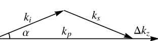
zFig. 2. The relation betweenαand∆kz sets a natural upper
bound toαfor near-collinear emission.
Γ 7
Γ 5
Γ 3
0.000 0.002 0.004 0.006 0.008 0.010
L
R 50100 150 200
K
Fig. 3.(Color online) The blue line (uppermost) is the gener-ation bandwidth defined in (12), the green curves (dashed) are calculated from our analytical treatment, and the red curves (solid) are the result of our geometrical argument.
4 Geometrical argument
In this section we find an upper (and therefore lower) bound for the generated OAM values, and for the mea-sured OAM values. The measurement bandwidth that we calculate from such bounds matches the analytic result of the previous section and therefore allows to avoid calcu-lating numerically the distribution of projection probabil-ities.
The phase-matching efficiency of the down-conversion process depends upon the axial mismatch ∆kz in wave vectors of the pump, signal and idler fields, and it is given by sinc2(L∆kz/2). When optimised for degenerate, near-collinear phase-matching, the signal and idler output is obtained over a narrow range of angles, α, for which L∆kzπ. With reference to Figure2, for smallα(which corresponds to being near to collinearity) we can write
∆kz≃ α2k
p
2 . (8)
It follows, therefore, that the allowed values of α are bounded from above:
α2 2π
kpL. (9)
[image:4.595.322.525.163.289.2]Page 4 of6 Eur. Phys. J. D(2012) 66: 178
generated OAM bandwidth. Such restriction is a natural consequence of the fact that a generated mode cannot be more divergent than the down-conversion cone. The rela-tionβα, using the definitions and bounds given above forβ andα, can be rewritten as
ℓr
πkp
2L, (10)
where we have made the approximation thatks,i ≈kp/2. This relation is the starting point to calculate the genera-tion bandwidth and for the analysis in the far field of the image plane of the crystal.
4.1 Generation bandwidth
The beam size can be no bigger than that of the pump beam, i.e. rwp. Applying this bound to equation (10) we obtain an upper bound for the generated OAM value:
ℓgenwp
πkp 2L =
π
LR
. (11)
It follows, therefore, that the generation bandwidth is
Kgen= 1 + 2
π
LR. (12)
This number represents the effective number of entangled OAM modes generated by the source obtained by remov-ing thep= 0 restriction (as we are applying such restric-tion only to the measurement bandwidth). Equivalently, it can be thought of as the bandwidth obtained by removing the restriction onγ, i.e. if one does detectp= 0, but with anyγ. This way of thinking aboutKgencan be helpful, as it relates to a measurement scheme. The relation between Kgen and the total Schmidt number K or its azimuthal partKaz [26] is not straightforward, becauseKgen can be thought of in terms of a measurement with any value ofγ.
4.2 Image plane bandwidth
As anticipated in Section 2, to calculate the measurement bandwidth we need to consider the overlap of the gener-ated field with the detection modes in the image plane of the crystal and in its far field. Intuitively, a detection system which has a good overlap in the image plane, but that detects light that only comes from a narrow spread of directions would restrict the measured bandwidth. A simi-lar restriction would occur for one that has a good overlap with the typical incoming angles of LG beams, but that has a poor overlap with the intensity in the image plane. It is clear that in order to optimise a detection system, both these quantities have to be taken into account.
To calculate the overlap in the image plane it suffices to note that ap= 0 Laguerre-Gaussian mode with OAM
number ℓ and width w has its maximum intensity at a radius
r=w
ℓ
2. (13)
For efficient conversion of pump to signal and idler we require that the pump, single and idler beams should all overlap, giving a restriction on the maximum size of the down-converted beams (rs,i wp) and hence an upper bound to the value of OAM in the plane of the crystal corresponding to
rs,i =ws,i
ℓ
2 wp. (14)
In terms of γ, this gives an upper bound of the value of the OAM in the plane of the crystal:
ℓip2γ2 (15)
and hence an image plane bandwidth
Kip= 1 + 4γ2. (16)
4.3 Far field bandwidth
It is clear that in the far field of the plane of the crystal, instead of a real space argument, we need to use the angu-lar relationshipβ α, expressed in (10), where we apply the restriction for the maximum width of the detection modes given in (14):
ℓws,i
ℓ 2
πkp
2L. (17)
From which, replacingws,iwithwp/γ, we obtain an upper bound of the value of the OAM in the far field of the plane of the crystal:
ℓFF
π 2γ2L
R
(18)
and therefore a far field bandwidth
KFF = 1 +
π γ2L
R. (19)
4.4 Measurement bandwidth
If Kip and KFF are very different from each other, the resulting measurement bandwidth is given by the smaller of the two. For cases where the bandwidths are similar it is sensible to combine them. The convolution of two normal distributions of widths k and k′ gives a normal distribution of width (k−2+k′−2)−1/2. Similarly, we can get an estimate of the total measurement bandwidth by considering the convolution of two normal distributions of widths Kip and KFF. The bandwidth of the resulting distribution is
K= K−2
ip +K
−2 FF
−1/2
=
1 + 4γ2−2 +
1 + π
γ2L R
−2−1/2
5 Analysis of the results
For a comparison between the analytic and geometric ar-guments, we calculate the width of the distribution given by the modulus squared of the coefficients in (6) and com-pare it to (20). In Figure3 we plot the two bandwidths as functions of LR for γ = 3, γ = 5 and γ = 7. The solid curves (red online) represent the measurement band-width calculated from the numerical evaluation of the an-alytical model. The dashed curves (green online) are the same bandwidths calculated with our geometrical argu-ment. The uppermost solid line (blue online) is the gen-eration bandwidth. Note that to achieve high dimensional entanglement the crystal length should be a small fraction of the Rayleigh range.
We see that the geometrical argument is in excellent agreement with the numerical evaluation of our analytical result. The effect of increasingγyields a higher measure-ment bandwidth for very small values ofLR, but for large enough values of γ and for fixed LR, the measurement bandwidth eventually drops. Therefore it reaches a maxi-mum value for a particular crystal length. Under all con-ditions the measurement bandwidth never reaches that of the generation bandwidth, because we are restricting the measurement to modes with p = 0. Note, however, that the full generation bandwidth does not arise explic-itly from additional values of the OAM but rather from entanglement in the radial quantum numberp.
Differentiation of equation (20) with respect to the crystal length gives an estimate of the value of γ cor-responding to the highest measurement bandwidth for a givenLR. In this way we find
γopt≈ 4
π
4LR. (21)
It is worth noting that for such value of γ we have that Kip=KFF =Kgen, whereKgen is defined in (12). There-fore in the optimal case we haveK=Kgen/
√
2.
We define short crystal lengths as LR ≪ π/4γ4, for which the generation bandwidth is large, meaning that the measurement bandwidth is dominated by the image plane overlap of the detection modes with the pump. This gives a measurement bandwidth of
K≈Kip= 1 + 4γ2. (22)
Note that this short crystal limit is characterised by an independence ofKon the crystal length. In fact, it can be seen in Figure3that the leftmost part of the measurement bandwidth curves is flat (for the γ = 7 curve this is not visible in this plot, but the slope of equation (20) near the origin is zero for anyγ), and that the range of values ofLR over which they stay flat is inversely proportional to γ4. For much longer crystals,LR≫π/4γ4, the measurement bandwidth, as modified by the limiting overlap in the far field, becomes dominant, giving
K≈KFF= 1 +
π LRγ2
. (23)
LR0.002
LR0.003
LR0.001
0
2
4
6
8
10
12
Γ
20
[image:6.595.327.516.91.222.2]40
60
80
K
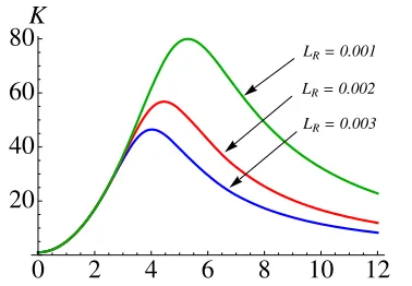
Fig. 4. (Color online) An example of a measurement band-width as a function ofγfor three different values ofLR: 0.001,
0.002 and 0.003 (highest to lowest).
In Figure4we plot three different curves, that describe the value of the measurement bandwidth as a function ofγ, for three different values of LR. Note that for each choice of LRthere is always an optimal value ofγwhich maximises K, and it corresponds to the optimal value given in (21). It is not an easy matter to determine the requisite parameters for existing experiments. Most our own exper-iments, however, correspond to values of γ in the range 1.5 up to about 4. In order to achieve higher degrees of entanglement in OAM, corresponding to larger Schmidt number, our analyses suggest that it would be desirable to press towards higher values ofγ.
6 Conclusions
We have shown two parameters determine the OAM band-width for entangled states produced by parametric down-conversion. These parameters are the ratio of the widths of pump and detection modesγ=wp/ws,i, and the crystal thickness normalised to the Rayleigh range of the pump LR=L/zr.
A simple geometrical argument approximates the ana-lytical results extremely well and allows us to suggest what needs to be adjusted in order to enhance the dimension-ality of the entanglement. We have restricted our analysis to a detection system that is sensitive to the LG p = 0 modes only. It is for this reason that the measurement bandwidth can never reach that of the generation band-width for any combination of parameters. It is possible, however, to identify an optimum value of γ to maximise the measurement bandwidth for any normalised crystal lengthLR.
Page 6 of6 Eur. Phys. J. D(2012) 66: 178
for financial support. SMB thanks Alison Yao for her invalu-able assistance with this manuscript.
References
1. M.A. Neilsen, I.L. Chuang, Quantum computation and quantum information (Cambridge University Press, Cambridge, 2000)
2. G. Molina-Terriza, J.P. Torres, L. Torner, Nat. Phys. 3, 305 (2008)
3. S.M. Barnett, Quantum information (Oxford University Press, Oxford, 2009)
4. F.M. Miatto, T. Brougham, A.M. Yao, Eur. Phys. J. D (2012),DOI: 10.1140/epjd/e2012-30063-y
5. L. Allen, S.M. Barnett, M.J. Padgett, Optical Angular Momentum(Institute of Physics Publishing, Bristol, 2003) 6. A.E. Siegman, Lasers (University Science Books,
Sausalito, 1986)
7. A. Mair, A. Vaziri, G. Weihs, A. Zeilinger, Nature 412, 313 (2001)
8. S. Franke-Arnold, S.M. Barnett, M.J. Padgett, L. Allen, Phys. Rev. A65, 033823 (2002)
9. J.P. Torres, A. Alexandrescu, L. Torner, Phys. Rev. A68, 050301 (2003)
10. J. Leach, B. Jack, J. Romero, A.K. Jha, A.M. Yao, S. Franke-Arnold, D.G. Ireland, R.W. Boyd, S.M. Barnett, M.J. Padgett, Science329, 662 (2010)
11. S.M. Barnett, D.T. Pegg, Phys. Rev. A41, 3427 (1990) 12. B.J. Pors, F. Miatto, G.W. ’t Hooft, E.R. Eliel, J.P.
Woerdman, J. Opt.3, 064008 (2011)
13. F.M. Miatto, A.M. Yao, S.M. Barnett, Phys. Rev. A 83, 033816 (2011)
14. B. Jack, A.M. Yao, J. Leach, J. Romero, S. Franke-Arnold, D.G. Ireland, S.M. Barnett, M.J. Padgett, Phys. Rev. A
81, 043844 (2010)
15. S.S.R. Oemrawsingh, X. Ma, D. Voigt, A. Aiello, E.R. Eliel, G.W. ’t Hooft, J.P. Woerdman, Phys. Rev. Lett.95, 240501 (2005)
16. A.C. Dada, J. Leach, G.S. Buller, M.J. Padgett, E. Andersson, Nat. Phys.7, 677 (2011)
17. J.T. Barreiro, N.K. Langford, N.A. Peters, P.G. Kwiat, Phys. Rev. Lett.95, 260501 (2005)
18. B.E.A. Saleh, M.C. Teich, Fundamentals of Photonics (Wiley, New York, 2007)
19. R.S. Bennink, Phys. Rev. A81, 053805 (2010) 20. A.M. Yao, New J. Phys.13, 053048 (2011)
21. C.K. Law, J.H. Eberly, Phys. Rev. Lett. 92, 127903 (2004)
22. J.B. Pors, S.S.R. Oemrawsingh, A. Aiello, M.P. van Exter, E.R. Eliel, G.W. ’t Hooft, J.P. Woerdman, Phys. Rev. Lett.
101, 120502 (2008)
23. J. Romero, J. Leach, M.R. Dennis, S. Franke-Arnold, S.M. Barnett, M.J. Padgett, Phys. Rev. Lett.106, 100407 (2011)
24. G. Watson,A Treatise on the Theory of Bessel Functions, Cambridge Mathematical Library (Cambridge University Press, 1995)
25. M.J. Padgett, L. Allen, Opt. Commun.121, 36 (1995) 26. M.P. van Exter, A. Aiello, S.S.R. Oemrawsingh, G.