Laminar flow in three-dimensional square–square expansions
P.C. Sousa
a, P.M. Coelho
b, M.S.N. Oliveira
a, M.A. Alves
a,⇑a
Departamento de Engenharia Química, CEFT, Faculdade de Engenharia da Universidade do Porto, Rua Dr. Roberto Frias, 4200-465 Porto, Portugal b
Departamento de Engenharia Mecânica, CEFT, Faculdade de Engenharia da Universidade do Porto, Rua Dr. Roberto Frias, 4200-465 Porto, Portugal
a r t i c l e
i n f o
Article history: Received 25 May 2010
Received in revised form 2 June 2011 Accepted 3 June 2011
Available online 13 June 2011
Keywords: Viscoelastic fluid Boger fluid Flow visualization PIV
3D expansion flow Numerical simulations
a b s t r a c t
In this work we investigate the three-dimensional laminar flow of Newtonian and viscoelastic fluids through square–square expansions. The experimental results obtained in this simple geometry provide useful data for benchmarking purposes in complex three-dimensional flows. Visualizations of the flow patterns were performed using streak photography, the velocity field of the flow was measured in detail using particle image velocimetry and additionally, pressure drop measurements were carried out. The Newtonian fluid flow was investigated for the expansion ratios of 1:2.4, 1:4 and 1:8 and the experimental results were compared with numerical predictions. For all expansion ratios studied, a corner vortex is observed downstream of the expansion and an increase of the flow inertia leads to an enhancement of the vortex size. Good agreement is found between experimental and numerical results. The flow of the two non-Newtonian fluids was investigated experimentally for expansion ratios of 1:2.4, 1:4, 1:8 and 1:12, and compared with numerical simulations using the Oldroyd-B, FENE-MCR and sPTT constitutive equations. For both the Boger and shear-thinning viscoelastic fluids, a corner vortex appears downstream of the expansion, which decreases in size and strength when the elasticity of the flow is increased. For all fluids and expansion ratios studied, the recirculations that are formed downstream of the square–square expansion exhibit a three-dimensional structure evidenced by a helical flow, which is also predicted in the numerical simulations.
Ó2011 Elsevier B.V. All rights reserved.
1. Introduction
The flow of Newtonian and non-Newtonian fluids in channels with variable cross-section, which include contractions and expan-sions, is a classical fluid mechanics problem, which has been ad-dressed in a number of experimental and numerical studies published in the literature (e.g.[1–7]). The investigation of these flows is essential not only from a fundamental point of view but also due to their importance in practical applications, namely in the polymer processing industry. The flow through sudden con-tractions is a benchmark problem that has received broader atten-tion than the flow through abrupt expansions, possibly due to the wide and interesting nature of the flow patterns that occur in con-traction flows, particularly with viscoelastic fluids (e.g. vortex enhancement, divergent and unsteady flow)[8], and its applicabil-ity to estimate the extensional viscosapplicabil-ity in entry-flows (e.g.[9,10]). Nevertheless, expansion flows can also be used to understand en-try-flow problems and to validate numerical codes.
Early experimental studies on expansion flows focused on Newtonian fluids in two-dimensional (2D) geometries[11–13]. It was found that Moffatt vortices[14] appear downstream of the
expansion and that flow inertia promotes the enhancement of these recirculations. Later on, Acrivos and Schrader[15]and Milos et al.[16]investigated numerically the flow of Newtonian fluids at high values of the Reynolds number (Re) and they found that above a critical value of Re the flow becomes unsteady. Furthermore, according to the experiments of Townsend and Walters[17]and the numerical predictions of Baloch et al.[18], a pair of lip vortices develops close to the re-entrant corner for high expansion ratios. These vortices then expand to the downstream wall increasing in size with the Reynolds number.
Townsend and Walters[17]have also studied the flow behavior of viscoelastic fluids through expansions, including the flow of a 0.15% aqueous solution of polyacrylamide (PAA) through 3:40 and 1:80 planar expansions, and the flow of a 0.1% aqueous solu-tion of xanthan gum and glass fibers through three-dimensional (3D) axisymmetric expansions (expansion ratio of 3:40). For visco-elastic fluids, the recirculations also appear downstream of the expansion, but unlike the Newtonian case, the recirculations de-crease in size when the elasticity of the flow is inde-creased. Baloch et al. [19] used the linear form of the Phan-Thien and Tanner (PTT) model[20,21]to numerically simulate a number of viscoelas-tic flows in planar (expansion ratio of 3:40 and 1:80) and 3D (expansion ratio of 3:3:40) geometries. In agreement with the experimental work of Townsend and Walters[17], the numerical results of Baloch et al. [19] reported a decrease in the vortex
0377-0257/$ - see front matterÓ2011 Elsevier B.V. All rights reserved. doi:10.1016/j.jnnfm.2011.06.002
⇑ Corresponding author. Tel.: +351 225081680; fax: +351 225081449. E-mail addresses:psousa@fe.up.pt (P.C. Sousa), pmc@fe.up.pt (P.M. Coelho), monica.oliveira@fe.up.pt(M.S.N. Oliveira),mmalves@fe.up.pt(M.A. Alves).
Contents lists available atScienceDirect
Journal of Non-Newtonian Fluid Mechanics
activity due to viscoelasticity, which pushes the recirculations against the downstream corners as previously described by Halmos and Boger[22]. In particular, the viscoelastic fluid flow through planar expansions shows a reduction of the vortex size and strength as the Deborah number (De) is increased. Eventually, at high Deborah number flows, the recirculations downstream of the expansion seem to disappear altogether. This suppression mechanism has been compared to the extrudate-swell phenome-non, in which the polymer molecules passing through an expan-sion and entering a larger cross-section reservoir relax the elastic stresses by expanding the main flow stream tube[23]. Another interesting feature worth mentioning is the onset of a lip vortex in the inlet channel upstream of the expansion observed for Upper-Convected Maxwell (UCM) and Oldroyd-B fluids flowing through a 1:3 planar expansion under creeping flow conditions [23]. More recently, the same authors investigated the effect of the expansion ratio on the flow patterns of a UCM fluid[24]. For the lower expansion ratios, a non-monotonic variation of vortex length withDewas predicted, with vortex reduction at lowDe, fol-lowed by vortex enhancement at higherDe. For high expansion ra-tios (ER > 3), the vortex size was found to decrease monotonically asDeincreases.
There are several works that report the development of asym-metric flow in planar expansions for Newtonian and
non-Newto-nian fluids (e.g. [25–31]). Cherdron et al. [25] used flow
visualization and laser-Doppler anemometry techniques to quan-tify the steady asymmetry that develops for the Newtonian flow in symmetric planar sudden-expansion geometries, and concluded that the intensity of fluctuating energy measured in such low Reynolds number flows can even be larger than that observed in corresponding turbulent flows. Fearn et al.[26]investigated exper-imental and numerically the Newtonian fluid flow through a symmetric sudden planar expansion (ER = 3) and found that the flow becomes asymmetric and time-dependent for high Reynolds numbers, and related this effect with the 3D structure that devel-ops under those conditions. For generalized Newtonian fluids there are also a number of works that investigate the effect of shear-thinning and shear-thickening effects on the critical conditions for development of flow asymmetries in planar sudden expansion flows. Manica and Bortoli[27]used a power-law model to study numerically the laminar flow in a 1:3 planar expansion, and con-cluded that for shear-thinning fluids the critical Reynolds number for onset of steady flow asymmetry increases as the power law in-dex (n) is reduced, while the opposite happens to shear-thickening fluids asnincreases. More recently, Neofytou[28]used Casson and power-law rheological models to investigate the laminar flow in a 1:2 planar expansion. For both non-Newtonian fluids the numeri-cal results showed a linear relation between the inverse dimen-sionless inlet wall shear stress, at the critical flow conditions for onset of asymmetry flow, and the corresponding dimensionless wall shear rate for the range of Power–Law index and Bingham numbers investigated.
There are also a few studies investigating the stabilizing effect of viscoelasticity on the critical conditions for onset of flow asym-metries in planar expansion flows. Oliveira[29]studied numeri-cally the flow of constant shear viscosity viscoelastic fluids (Boger fluids) through 1:3 planar expansions. The working fluids were a viscoelastic fluid that was described using the modified FENE-CR constitutive equation and a Newtonian fluid that was used with the purpose of validating the method and for compari-son purposes. The numerical results showed that the flow becomes asymmetric for both fluids, however, for the viscoelastic case, the elasticity tends to stabilize the flow and the critical Reynolds num-ber is higher than that found for a Newtonian fluid. More recently, Rocha et al.[30]also investigated the onset of asymmetries in vis-coelastic fluid flow through a 1:4 planar sudden expansion. The
authors determined the criticalReat which the bifurcation phe-nomenon occurs, and concluded that it is lower than that obtained for lower expansion ratios[29]. Asymmetries in the mean axial velocity profile of a shear-thinning fluid flowing through an axi-symmetric abrupt expansion were also found in the work of Dales et al.[32]in which the fluid was an aqueous solution of PAA and the flow regime was turbulent. However, in this case, the Newto-nian fluid (water) flow did not show any asymmetries. More re-cently, another experimental study [33] showed that for a 1:2 axisymmetric expansion the Newtonian fluid flow also becomes asymmetric (and steady), under laminar flow conditions, above Re= 1139. For Re> 1400 the flow eventually becomes time-dependent.
In most of the planar expansion flows discussed above, three-dimensional effects are negligible and less demanding 2D numeri-cal simulations can be used to predict the flow correctly. Configu-rations where three-dimensional effects are important are more challenging to analyze experimental and numerically and as such, the number of published works concerning this topic is reduced. Two important exceptions are the works of Burgos and Alexandrou [34]and Alexandrou et al.[35]in which the flow of a generalized non-Newtonian fluid (Herschel-Bulkley) through three-dimen-sional 1:2 and 1:4 expansions was investigated. In the first work [34], the unsteady flow in a 1:2 sudden expansion was studied and in the latter[35], the steady flow of Herschel-Bulkley fluids was investigated. The authors showed that the development of yielded and unyielded regions in this type of 3D geometries de-pends on the expansion ratio and on Bingham and Reynolds numbers.
In this work, we focus on the flow through a three-dimensional square–square expansion, with different expansion ratios (ER = 2.4, 4, 8 and 12, defined as the ratio between the side lengths of the downstream and upstream square ducts). We use Newtonian and viscoelastic fluids with different rheological characteristics: a Boger fluid, for which the shear viscosity is nearly independent of the shear rate and a shear-thinning viscoelastic fluid. Visualiza-tions were undertaken in order to assess the flow patterns and detailed particle image velocimetry (PIV) measurements were per-formed to quantify the velocity field. For the Boger fluid, pressure drop measurements are also presented and discussed. Moreover, 3D numerical simulations were carried out in order to predict the Newtonian and non-Newtonian fluid flow through square– square expansions.
2. Experimental techniques
2.1. Experimental set-up
A scheme of the experimental set-up is shown inFig. 1. The main test section in the experimental rig has a square cross-section of lengthL= 1.75 m, which is composed of a downstream square channel, with a side length of 2H2= 24.0 mm, and an upstream
interchangeable square channel which fits inside the larger one and has a smaller side length. The internal side length of the inner square part can be set to 2H1= 10.0, 6.0, 3.0 or 2.0 mm in order to
obtain the desired expansion ratios, ER =H2/H1= 2.4, 4, 8 or 12.
The upstream and downstream sections are denoted by sub-scripts 1 and 2, respectively. For optical access, the channels are made of transparent perspex.
passage of the valve. The right-hand side reservoir was used to supply the fluid that flowed through the column, and it was placed on a weighing scale (KERN DS 16k0.2; with readout of 0.2 g and maximum range of 16 kg) in order to measure the mass flow rate (QmDWeight=Dtime). More details of the experimental set-up can be found in Ref.[8].
2.2. Measurement techniques
Two different optical techniques were used in this study, in or-der to characterize the flow field: streak photography and particle image velocimetry. For this purpose, the fluids used in the experi-ments were seeded with 10
l
m PVC tracer particles.Streak photography uses long time exposures to obtain a visual fingerprint of the flow patterns. For flow illumination, we used a 635 nm 5 mW laser diode (Vector, model 5200-20) or a 532 nm 3 mW laser diode (Imatronic, model LLM115). In both cases a cylindrical lens is attached to the diode to generate a sheet of light. The streak images were captured using a digital camera (Canon EOS 30 D) with a macro lens (Canon EF100 mm, f/2.8), placed per-pendicularly to the light sheet.
For the measurement of the velocity field, a doubled pulsed Nd:YAG laser, with a maximum energy of 50 mJ (Solo PIV III from New Wave Research) was used. The laser was combined with appropriate optical components, producing a planar light sheet that illuminates the plane under study. The images were recorded using a digital CCD camera (Flow Sense 2 M from Dantec Dynamics equipped with a Nikon AF Micro Nikkor 60 mm f/2.8D lens) which was placed perpendicularly to the light sheet. The images were processed using FlowManager v4.60 software (Dantec Dynamics) and the velocity vector map for each pair of images was deter-mined using a cross-correlation technique. A detailed discussion of the technique employed can be found in Ref.[36].
The flow visualizations and the velocity field measurements using PIV were both undertaken at different parallel planes of the flow in the square channel. Therefore, it was necessary to translate simultaneously the light source and the camera utilized for each optical technique using for this purpose a x–y traverse and a dial comparator (readout of ±0.01 mm).
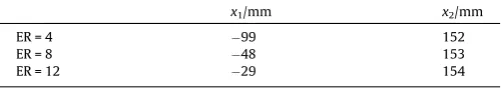
Pressure drop measurements across the expansion were carried out using differential pressure sensors (Honeywell, model 26PC series), previously calibrated using a hydrostatic column of water, which are able to cover pressure differences up to 6.9 kPa. The experiments were performed by determining the pressure drop (Dp) across the expansion, with one pressure port located up-stream (p1) and another port (p2) located downstream of the
expansion plane. The precise locations of the pressure ports are listed inTable 1for different ER.
For each flow rate studied, the output signal of the pressure transducer was recorded using LabView v7.1 software, until the steady-state was reached.
2.3. Rheological characterization
A Newtonian and two different non-Newtonian fluids were used in the experiments. Table 2 summarizes the composition and density (
q
) of the fluids, measured at 293.2 K using two hyd-rometers (readability of 1 kg/m3; ranges 1100–1200 kg/m3 and1200–1300 kg/m3). A biocide (Kathon LXE, Rohm and Haas) was added to the solutions, at a weight concentration of 25 ppm, in or-der to minimize bacterial growth and biological degradation of the fluids.
Furthermore, the working fluids were characterized rheologi-cally at different temperatures in the range of 283.26T/
K6303.2 using a shear rheometer (MCR301, Anton Paar) and the
time-temperature superposition method was used to obtain a mas-ter flow curve.
The variation of the viscosity with temperature can be de-scribed using an Arrhenius equation[37],
Electric winch
Outlet tank
Feed tank
Vacuum pump
Scale Flow
direction
Laser diode Tubes
2
H
22
H
1Expansion plane Air line
x
[image:3.595.155.454.69.306.2]Computer
Fig. 1.Schematic diagram of the experimental set-up.
Table 1
Pressure port locations in thex-direction (streamwise) for each expansion ratio. The expansion plane is located atx= 0.
x1/mm x2/mm
ER = 4 99 152
ER = 8 48 153
[image:3.595.312.563.710.754.2]lnðaTÞ ¼
D
H R 1 T 1 T0ð1Þ
whereaTis the shift factor,DHis an activation energy,Ris the uni-versal gas constant,Tis the absolute temperature of the measure-ment andT0is the absolute reference temperature, which is set
here asT0= 293.2 K, the temperature at which the experiments in
the square–square expansion were performed. The shift factor is de-fined as[37],
aT¼
g
ð TÞg
ðT0Þ T0T
q0
q
ð2Þwhere
g
(T) andq
are the shear viscosity and the fluid density at temperatureTandg
(T0) andq
0are the shear viscosity and the fluiddensity at the reference temperatureT0. Since the range of
temper-atures of the measurements is small, the shift factor can be simpli-fied to:
aT¼
g
ðTÞg
ðT0Þð3Þ
For the Newtonian fluid, the shear viscosity at the reference temperature is
g
(T0) = 0.0982 Pa s and DH/R= 5580 K. For thenon-Newtonian fluids we present inFig. 2the master curves mea-sured for steady shear flow. For the Boger fluid, we obtainedDH/ R= 6780 K for the range of temperatures between 283.2 and 303.2 K.
3. Numerical method and computational meshes
The flow through square–square expansions with different expansion ratios (ER = 2.4, 4, 8 and 12) was simulated numerically using a fully-implicit finite-volume method with a time marching pressure-correction algorithm[38]. The governing equations that
describe an isothermal, laminar and incompressible fluid flow are those of conservation of mass and momentum,
r
u¼0 ð4Þq
@u@tþ
r
uu
¼
r
pþg
sr
2uþ
r
s
ð5Þwhereuis the velocity vector,tthe time,pthe pressure and
g
StheNewtonian solvent viscosity. The extra-stress tensor (
s
t) is de-scribed by the sum of a Newtonianðss
¼g
sðruþruTÞÞand apoly-meric solute contribution (
s
). In the numerical simulations of the Newtonian fluid flow, the polymeric contribution to the extra-stress tensor is null (rs
¼0) and only the Newtonian component re-mains in Eq.(5). On the other hand, for the numerical simulations of the viscoelastic fluid flow, the polymeric contribution is included and is described using an appropriate rheological constitutive equa-tion. The following general equation was used,fðTr
s
Þs
þ k gðTrs
Þ@
s
@tþr
us
¼
g
Pru
þru
Tþ kgðTr
s
Þs
ru
þru
T
s
ð6Þwherekis the relaxation time,
g
Pis the zero-shear viscosity of thepolymer andfðTr
s
ÞandgðTrs
Þare functions of the trace of tensors
, Tr(s
).For the shear-thinning fluid the simplified PTT model was used (hereafter designated as sPTT model), which is obtained setting gðTr
s
Þ ¼1 and considering the linear form for the stress function f(Trs
),fðTr
s
Þ ¼1þke
gP
Trðs
Þ ð7Þwhere
e
is the extensibility parameter. For the Boger fluid two mod-els were used in the numerical simulations, namely the Oldroyd-B model and the FENE-MCR constitutive equation[39,40]. The Old-royd-B model has the known drawback of predicting an unbounded steady-state extensional viscosity above a critical dimensionless strain rate (ke
_crit¼0:5) and is obtained consideringe
¼0 (i.e. fðTrs
Þ ¼1) andgðTrs
Þ ¼1 in Eq.(6). The FENE-MCR model is ob-tained settinge
¼0 in Eq.(6), and considering the following stretch function,gðTr
s
Þ ¼L2
þ ðk=
g
PÞTrðs
ÞL23 ð8Þ
where the dimensionless parameterL2represents the ratio between the maximum and the equilibrium average dumbbell extensions. For large values ofL2the Oldroyd-B model is asymptotically
ap-proached, while using finite values ofL2removes the unbounded behavior of the steady-state extensional viscosity at large strain rates.
[image:4.595.30.555.90.134.2]For the shear-thinning fluid flow, the numerical simulations were performed using the sPTT model with one mode and a solvent contribution[20,21]. The model parameters were set by fitting the steady shear flow curve obtained experimentally (cf.Fig. 2), using the following parameters [41]: zero-shear polymer viscosity,
g
P= 1.62 Pa s; solvent viscosity,g
S= 0.03 Pa s; relaxation time,Table 2
Composition by weight and density of the fluids measured at 293.2 K.
Fluid PAA [ppm] Glycerin [%] Water [%] Kathon [ppm] NaCl [%] q[kg m3
]
Newtonian – 84.99 15.01 25 – 1221
Boger 100 90.96 7.52 25 1.51 1249
Shear-Thinning 600 59.94 40.00 25 – 1156
1E-3 0.01 0.1 1 10 100 1000 10000 0.01 0.1 1 10 100 0.01 0.1 1 10 B
(
η B/
a
T
) / Pas
(iB)
(
ηA
/
a
T) / Pas
a
Tγ.
/ s
-1(iA)
[image:4.595.41.270.123.314.2]A 0.001 283.2 K 288.2 K 293.2 K 298.2 K 303.2 K Elastic instability 0.001
Fig. 2.Master curves of the steady shear viscosity measured at different
k= 32 s; extensibility parameter,
e
= 0.06. This fit is also shown in Fig. 2for comparison with the experimental data.For the Boger fluid flow, simulations were carried out using both the Oldroyd-B and the FENE-MCR models with the following parameters:
e
= 0, k= 3.29 s,g
P= 0.279 Pa s andg
S= 0.367 Pa s.These parameters were selected based on the fit of a three-mode model with a solvent contribution to the rheological measure-ments obtained under small amplitude oscillatory shear flow, as detailed in our previous work[8]. For the simulations using the FENE-MCR model a value ofL2
¼100 was used (in agreement with other works in the literature, e.g.[40]), although in some cases the influence ofL2was also analyzed.
Eqs.(4)–(6)are integrated in space over the computational cells of the mesh and in time over a small time step (dt). The time deriv-ative is discretized with an implicit first-order Euler scheme, the diffusive terms are discretized with second-order central differ-ences and the discretization of the advective terms, both in the momentum and constitutive equations, is done using the CUBISTA high-resolution scheme[42].
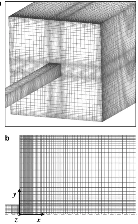
The computational meshes used in this study for the numerical simulation of the flow through square–square expansions are composed of three-dimensional orthogonal blocks and non-uni-form cells that follow a geometrical progression within each direction. For the expansion ratios of 2.4, 4 and 8, the numerical simulations were carried out using three different meshes: mesh M40 which has 40 cells iny- andz-directions of the downstream channel, mesh M64 with 64 cells in y- and z-directions and a more refined mesh, M80 which has 80 cells in both orthogonal directions. For the expansion ratio of 12, simulations were per-formed using three meshes with a slightly different number of cells: mesh M48, M60 and M96, which have 48, 60 and 96 cells in the y- and z-directions of the downstream channel, respec-tively. The total number of cells (NC) and the dimensionless min-imum cell size (Dxmin/2H2, Dymin/2H2 and Dzmin/2H2) of the
meshes used for all the ER are presented inTable 3. InFig. 3we show mesh M64 used in the numerical simulations of the flow through the 1:8 square–square expansion.
In spite of the geometrical symmetry relative to the central planes (y= 0 andz= 0) and diagonal planes (z= ±y), all simulations were performed on meshes covering the whole wall-to-wall geom-etries. Regarding the boundary conditions, no-slip condition at the solid walls was imposed and the inlets and outlets were positioned far from the expansion plane so that fully developed flow condi-tions were enforced. At the outlets, vanishing stream wise gradi-ents of velocity and extra-stress tensor compongradi-ents are imposed, and pressure is linearly extrapolated from the two upstream cell center values.
4. Flow patterns and vortex length
The flow of the Newtonian and viscoelastic fluids through square–square expansions, with different expansion ratios, was investigated in terms of the vortex length and flow patterns for a wide range of flow rates. For this purpose, different parallel planes of the channel were investigated using flow visualization.
4.1. Inertial effects
In order to study the influence ofReon the vortex dynamics of Newtonian fluid flow, visualizations of the flow patterns near the expansion plane were performed for a wide range of flow rates (Re< 20) and various expansion ratios (ER = 2.4, 4 and 8). Here, the Reynolds number is based on upstream flow characteristics and defined asRe=
qU
1(2H1)/g
, whereU1is the average velocityin the upstream channel. For the shear-thinning fluid, the viscosity is calculated using the sPTT model at a characteristic shear-rate (
c
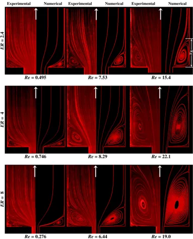
_ ¼U1=H1).InFig. 4we compare the experimental and numerical flow pat-terns obtained at the center plane for all expansion ratios studied. The numerical predictions were carried out with the refined mesh (M80) in order to ensure high accuracy.
[image:5.595.329.551.66.425.2]As can be observed inFig. 4, a Moffatt vortex[14]is formed downstream of the expansion plane, for all expansion ratios. Increasing the flow inertia leads to an increase of the vortex size Table 3
Characteristics of the computational meshes used (NC: number of computational cells).
ER Mesh NC Dxmin/2H2 Dymin/2H2=Dzmin/2H2
M40 164000 2.08102 2.04
102 2.4 M64 419840 1.39102
1.25102 M80 656000 1.03102
9.93103
M40 51000 1.31102
1.45102 4 M64 130560 8.20103
8.16103 M80 408000 6.26103 6.25
103
M40 163200 7.50103
8.69103 8 M64 417792 4.69103
4.55103 M80 652800 3.75103
3.75103
M48 113664 1.08102
9.52103 12 M60 177600 8.61103 8.33
103 M96 909312 1.34103
1.35103
Fig. 3.Zoomed view of mesh M64 used in the numerical simulations of the flow
[image:5.595.42.292.605.754.2]and an excellent agreement between the experimental results and numerical predictions is found. For Newtonian fluids, the forma-tion and dynamics of the recirculaforma-tions that appear downstream of an abrupt expansion is well-documented in the literature (e.g. [17,18,24,25]).
InFig. 5we analyze the effect of flow inertia on the measured normalized vortex length, xR/(2H2) (c.f. Fig. 4, Re= 15.4 and
ER = 2.4) for the Newtonian fluid. Moreover, we also present the numerical predictions obtained with the three meshes (M40, M64 and M80) used for each expansion ratio.
For all expansion ratios studied, the vortex size increases mono-tonically when the Reynolds number is increased. For the whole range ofRestudied, the numerical results obtained using meshes M40, M64 and M80 are in good agreement with the experimental results. Furthermore, the differences between the three meshes are small and the highest deviation between the results obtained is be-low 2%, demonstrating the high accuracy of the numerical simulations.
For creeping flow conditions (i.e. in the limit whenRe?0) the numerical simulations predict the following vortex dimensions:xR/
(2H2) = 0.141 for ER = 2.4; xR/(2H2) = 0.163 for ER = 4; xR/
(2H2) = 0.174 for ER = 8. These results are in agreement with the
predictions for square–square contraction flows under creeping flow conditions (cf.[8,43,44]), a consequence of the reversibility of Newtonian inertialess flows, i.e. in the limit when Re?0 the
flow patterns for expansion and contractions flows are
indistinguishable.
4.2. Elastic effects
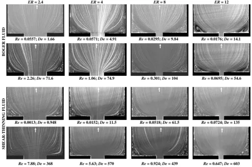
In order to quantify the effect of viscoelasticity, we use the Deborah number, here defined based on upstream flow conditions, De=kU1/H1.Fig. 6shows the flow patterns for both viscoelastic
[image:6.595.100.484.64.539.2]flu-ids obtained experimentally at the middle plane (y= 0 orz= 0), for a range of Deborah numbers (or flow rates), covering the whole range of ER studied.
Comparing the flow patterns for both viscoelastic fluids, several similarities can be identified. For all expansion ratios studied, the flow of the two viscoelastic fluids presents a corner vortex down-stream of the expansion plane and, in general, increasing the Deborah number leads to a decrease of the corner vortex length.
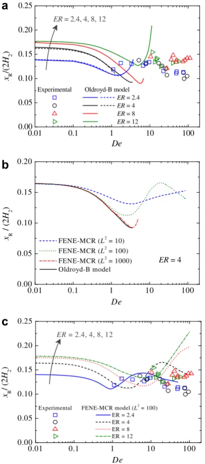
The dependence of the vortex length on the Deborah number, for all expansion ratios studied, is quantified inFig. 7for the Boger fluid and inFig. 8for the shear-thinning fluid. The vortex length is
scaled with the side length of the downstream square duct (2H2).
In addition, inFigs. 7 and 8we also show the predictions obtained from the numerical simulations.
For the lower expansion ratios, ER = 2.4 and 4, the numerical predictions of the viscoelastic fluid flow were obtained using meshes M64 and M80 and there is a good agreement between the numerical results using both computational meshes, as shown in Figs.7a and8. For this reason, and since the computational time required for the runs with more refined meshes is substantially higher, for the simulations of the viscoelastic fluid flow through the 1:8 and 1:12 square–square expansions we used only meshes M64 or M60, respectively. Note that besides the high relaxation times used, particularly for the shear-thinning fluid, the increase of the number of cells for the refined meshes (e.g. for ER = 12, the more refined mesh, M96, has five times more cells than mesh M60) renders the simulations of the viscoelastic fluid flow through 3D expansions with a high expansion ratio unfeasible in practice due to the very large CPU times involved (of the order of weeks for the highestDe).
At low Deborah numbers the numerical simulations predict accurately the creeping flow Newtonian plateaus for all fluids and expansion ratios (xR/(2H2) = 0.141 for ER = 2.4; xR/(2H2) =
0.163 for ER = 4; xR/(2H2) = 0.174 for ER = 8; xR/(2H2) = 0.177 for
ER = 12), which are not evident from the experimental results (cf. Figs.7a and8). The comparison between the experimental results obtained with the Boger fluid and the numerical simulations using the Oldroyd-B model is displayed inFig. 7a. The experimental data show a slight decrease of the vortex size with increasingDe, in con-trast with the numerical simulations that display vortex
suppres-sion only up to De1.5 and De6 for ER = 2.4 and 12,
0 2 4 6 8 10 12 14 16 18 20 0.00
0.25 0.50 0.75 1.00 1.25
ER = 8
ER = 4
x
R/(2
H
2)
Re
[image:7.595.63.277.65.226.2]ER = 2.4
Fig. 5.Dimensionless vortex length for Newtonian fluid flow as a function of the
[image:7.595.50.553.408.741.2]Reynolds number for ER = 2.4, 4 and 8. The symbols represent the experimental data, the dashed lines represent the numerical predictions performed using mesh M40, the thin solid lines the numerical results obtained with mesh M64 and the thick solid lines the predictions using the more refined mesh, M80.
respectively. At higher De significant vortex enhancement is predicted with the Oldroyd-B model, a phenomenon that is not reproduced in the experiments. Also, the convergence of the numerical simulations using the Oldroyd-B model is limited to a range ofDesignificantly narrower than that achieved in the exper-iments. To enhance the numerical stability, we also performed numerical simulations using the FENE-MCR constitutive equation. As detailed in Section 3, the values of parametersk,
g
Pandg
Softhe FENE-MCR model were the same as in the Oldroyd-B model. However, we were unable to select the appropriate value of L2 based on steady or oscillatory shear data alone, and as such a base value ofL2
¼100 was chosen in agreement with previous studies
(e.g. [40]). To analyze the effect ofL2 on the numerical results,
we show inFig. 7b the vortex size predicted for ER = 4 and a wide range ofL2 values (from a relatively low value ofL2¼10 up to L2¼1000). For highL2(e.g. L2¼1000), the numerical results are similar to those obtained with the Oldroyd-B model, with very lit-tle improvement in terms of numerical stability and therefore in terms of the range ofDewe are able to achieve in the simulations. On the other hand, for lowL2(e.g.L2
¼10) the polymer molecules do not stretch significantly, and therefore elastic effects are sup-pressed, with a low influence ofDeon the vortex size. For interme-diate L2 values, we are able to observe a more pronounced
influence ofDeon the flow characteristics. ForL2
¼100 an inter-esting behavior is observed in the predicted vortex size, with a minimum vortex size occurring atDe2.5, followed by a maxi-mum value atDe20. This non-monotonic behavior is exclusively due to the elasticity of the fluid, since inertial effects are negligible, even at the largerDeflow conditions. Indeed, for the higher flow rate cases we performed additional flow simulations assuming the limiting behavior of creeping flow (by dropping the convective term in the momentum equation) and the differences observed rel-ative to the inertial case are negligible (in all cases below 1%), con-firming that inertia is not important here. We also note that the normal stresses are maximum along the upstream channel walls, and in the vicinity of the expansion plane corner (singularity), and the numerical simulations show an increase of Tr(
s
) whenL2increases.
InFig. 7c we compare the experimental measurements of vor-tex length for the various ER investigated with the predictions using the FENE-MCR model, assumingL2¼100, a value used here-after in all the numerical simulations with the FENE-MCR model. The agreement between experiments and numerical simulations is now better than that found for the Oldroyd-B model, but still there are significant differences, indicating that more realistic con-stitutive equations are needed to better reproduce the behavior of the Boger fluid, probably using multimode models.
For the shear-thinning fluid, the decrease of the vortex size with Deis more pronounced, in particular for the lower expansion ra-tios, as is visible in the experimental data shown inFig. 8. The pre-dictions using the sPTT model are restricted to a significantly narrower range of De, as compared with the experiments, and the vortex reduction trend is only predicted at lowDeflow condi-tions. Interestingly, the same shear-thinning fluid was used in Ref.[41]to investigate the viscoelastic flow in square–square con-tractions[41], but in that case a much better agreement between
0.01 0.1 1 10 100
0.00 0.05 0.10 0.15 0.20 0.25
Experimental Oldroyd-B model
ER = 2.4
ER = 4 ER = 8
ER = 12
x
R/(2
H
2)
De
ER = 2.4, 4, 8, 12
0.01 0.1 1 10 100
0.00 0.05 0.10 0.15 0.20
FENE-MCR (L2 = 10)
FENE-MCR (L2 = 100)
FENE-MCR (L2
= 1000) Oldroyd-B model xR / ( 2 H2 ) De
ER = 4
0.01 0.1 1 10 100
0.00 0.05 0.10 0.15 0.20 0.25
ER = 2.4, 4, 8, 12
[image:8.595.326.526.68.215.2]Experimental FENE-MCR model (L2 = 100) ER = 2.4 ER = 4 ER = 8 ER = 12 xR / (2 H2 ) De
a
b
c
Fig. 7.Dimensionless vortex length as a function of the Deborah number for Boger
fluid flow. (a) Comparison of experimental data (symbols) with predictions using the Oldroyd-B model for different ER (solid lines represent the numerical predictions using mesh M64 for ER = 2.4, 4 and 8 or mesh M60 for ER = 12, and the dashed lines represent the numerical predictions using mesh M80 for ER = 2.4 and 4); (b) Influence of parameterL2
of FENE-MCR model for ER = 4 (mesh M64); (c) Comparison between FENE-MCR predictions (L2= 100) and experimental results for different ER (meshes M60 for ER = 2.4, 4 and 8; mesh M64 for ER = 12).
0.01 0.1 1 10 100 1000
0.00 0.05 0.10 0.15 0.20 0.25
ER = 2.4, 4, 8, 12
ER = 2.4
ER = 4
ER = 8
ER = 12
x
R/(2
H
2)
De
Fig. 8.Dimensionless vortex length as a function of the Deborah number for the
[image:8.595.58.262.69.529.2]the experiments and the numerical simulations (also using the sPTT model with the same parameters used in the present investi-gation, and the same viscoelastic flow solver) was observed with converged numerical simulations in a wider range ofDe, showing that the expansion flow is a numerically more stringent flow problem.
4.3. Three-dimensionality of the flow
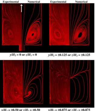
The previous investigations regarding the flow of Newtonian and viscoelastic fluids, through square–square contractions [8,43,44], demonstrated that the flow in these geometries is highly three-dimensional. In order to study the 3D nature of the flow through square–square expansions, a detailed investigation at sev-eral parallel planes was carried out.Fig. 9shows the visualized pathlines and the corresponding numerical predictions for the Newtonian fluid flow at different planes of the 1:8 square–square expansion, ranging from the center plane (y/H2= 0 orz/H2= 0) to
a plane near the wall of the channel (y/H2= ±0.875 or z/ H2= ±0.875). At the center plane the pathlines illustrated are real,
while for the other planes the visualized flow shows the projec-tions of the pathlines at the visualized plane. Again, we observe an excellent agreement between the visualizations and the numer-ical predictions.
For the range of flow rates studied, the flow is symmetric rela-tive to the two center planes (y= 0 andz= 0) and to the two diag-onal planes (y= ±z). To further document the complex flow
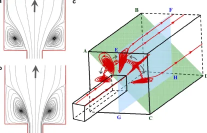
behavior in square–square expansions, in Fig. 10 we show a three-dimensional view of some streamlines, showing the open vortical structures predicted numerically with the refined mesh (M80) for the Newtonian fluid at creeping flow conditions (Re?0 and CR = 4). To simulate creeping flow conditions we ne-glect the convective term in the momentum equation, but keep the transient termð
q@u=@t
Þand use a pseudo-time marching algo-rithm to achieve steady flow conditions. When steady-state is achieved, the transient term vanishes, and we obtain exactly creep-ing flow conditions (Re= 0). [image:9.595.145.459.372.736.2]Under creeping flow, the streamlines generated by the Newtonian fluid flowing through a square–square expansion are coincident with those documented previously for the flow through square–square contractions[8,43,44] due to the revers-ibility of inertialess flows. However, in the present configuration the flow occurs in the opposite direction, causing the fluid that is flowing near the center plane wall of the upstream channel to pass through the expansion plane and enter the recirculation in the center plane (plane EFGH in Fig. 10c). Once there, the fluid rotates around the center of the recirculation and follows a heli-cal trajectory toward the diagonal plane (ABCD), where it turns now to the periphery and exits the recirculation moving toward the exit of the downstream channel close to the diagonal plane wall, as illustrated in Fig. 10c. The streamlines in the center and diagonal planes are shown in Fig. 10a and b, respectively, to better illustrate the dynamics of the secondary flow in the symmetry planes.
Interestingly, when inertial effects are important, besides the increase of the recirculation documented previously (cf. Figs. 4 and 5) we observe a reversal in the flow direction within the recir-culation. This can be observed in the streamlines plotted inFig. 11 at Re= 10 and CR = 4. In this case, the recirculating flow occurs from the diagonal planes, where the fluid is sucked in (cf. Fig. 11b), to the center planes where the fluid is ejected (cf. Fig. 11a). Such a flow reversal was previously documented in
square–square contractions, but was attributed to elastic effects [8,43,44]. The present results suggest that flow reversal in square–square contractions or expansions is not a fingerprint of elastic effects, but seems to occur concomitantly with vortex enhancement, which is inertially-driven in expansion flows and elasticity-driven in contraction flows.
In Fig. 12 we show pathline projections of the Boger and shear-thinning fluid flows at different parallel planes of the 1:2.4
Fig. 10.Streamlines predicted numerically for the Newtonian fluid flow through the 1:4 square–square expansion under creeping flow conditions (Re?0). (a) Streamlines at
the center plane (EFGH); (b) streamlines at the diagonal plane (ABCD); (c) three-dimensional view of some streamlines. Note that in the center planes (a) the fluid enters the recirculation while in the diagonal planes (b) the fluid exits the recirculation.
Fig. 11.Streamlines predicted numerically for the Newtonian fluid flow through the 1:4 square–square expansion atRe= 10. (a) Streamlines at the center plane (EFGH); (b)
square–square expansion and identical Deborah numbers, illustrating the complex and highly three-dimensional flow behavior particularly near the walls.
5. Velocity field
5.1. Newtonian fluid
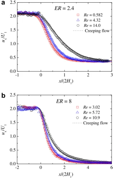
[image:11.595.99.506.67.313.2]In order to highlight the inertial effects on the velocity field, in Fig. 13we show axial velocity profiles along the centerline for two expansion ratios (ER = 2.4 and ER = 8), at different Reynolds num-bers. The axial velocity profile predicted numerically for negligible inertial flow conditions (creeping flow) is also shown for compar-ison purposes. Moreover, we compare the experimental results with numerical predictions for each value ofRe.
In all cases, the dimensionless velocity profiles are plotted from locations upstream (x< 0) to downstream (x> 0) of the expansion plane. As can be seen, the dimensionless velocity gradient down-stream of the expansion plane decreases when the Reynolds num-ber increases. As inertia increases, entrance effects also become more pronounced and the size of the recirculations, formed down-stream of the expansion plane, also increases. For ER = 2.4, the nor-malized velocity profile measured experimentally at low Re is similar to that obtained numerically for creeping flow. For all axial velocity profiles shown inFig. 13, the experimental results are in good agreement with those predicted numerically, for both ER = 2.4 and 8, thus validating the PIV measurements.
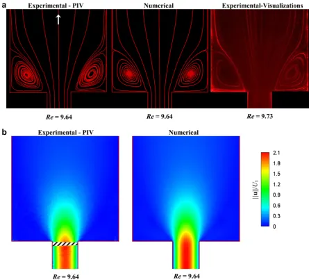
To further attest the good agreement between experimental and numerical results, inFig. 14a we present a comparison be-tween the middle plane pathlines obtained using three different approaches: flow visualizations using streak photography; integra-tion of the measured velocity field using PIV; numerical predic-tions. The example shown corresponds to Newtonian fluid flow through the 1:4 square–square expansion at similar Reynolds numbers (Re10). InFig. 14b we compare the normalized velocity magnitude contour plots obtained from the PIV measurements and from the numerical simulations. Again, the experimental results are in excellent agreement with the numerical predictions.
5.2. Viscoelastic fluid
Fig. 15shows normalized axial velocity profiles taken along the centerline for the Boger fluid flowing through the 1:4 and 1:12
Fig. 12.Projections of pathlines at different parallel planes for the Boger (a) and shear-thinning (b) fluid flow through the square–square expansion (ER = 2.4).
-1 0 1 2 3
0.0 0.5 1.0 1.5 2.0 2.5
Re = 0.582
Re = 4.32
Re = 14.0
Creeping flow
u
x/
U
1x
/(2
H
1)
ER
= 2.4
-2 0 2 4 6
0.0 0.5 1.0 1.5 2.0 2.5
Re = 3.02
Re = 5.72
Re = 10.9
Creeping flow
u
x/
U
1x
/(2
H
1)
ER
= 8
a
[image:11.595.338.536.353.665.2]b
Fig. 13.Experimental (symbols) and numerical (lines) axial velocity profiles at the
square expansions (Fig. 15a) and for the shear-thinning fluid flowing through square–square expansions with expansion ratios of 2.4 and 8 (Fig. 15b). Predictions of dimensionless velocity pro-files for a Newtonian fluid flowing at creeping flow conditions are also shown inFig. 15 to highlight the influence of elasticity on the dimensionless velocity profiles.
For a square channel, the theoretical maximum velocity or cen-terline velocity is 2.096 times the average velocity for a constant viscosity fluid (either Newtonian or a Boger fluid)[44]. Therefore, for the Boger fluid, the axial velocity far upstream of the expansion should beux/U1= 2.096 as observed for the computed profiles for
Newtonian and FENE-MCR fluids. In the limit De?0, obtained experimentally for very low flow rates, the axial dimensionless velocity profile approaches that of a Newtonian fluid under creep-ing flow conditions. An increase in the flow rate (orDe) leads to the appearance of a local maximum of the axial velocity near the expansion region, which is also predicted numerically using the FENE-MCR model, although with some differences observed due to the inability of this model to accurately reproduce the complex behavior of the Boger fluid. For the Boger and the shear-thinning fluids studied, at highDe, a significant overshoot on the axial velocity along the centerline is clearly visible with the maxi-mum axial velocity reaching values well above the fully-developed
value, which means that the fluid experiences an acceleration as it is approaching the expansion plane (converging streamlines) lead-ing to a higher rate of decay of the velocity when it enters the channel with larger cross-section. The same phenomenon was ob-served experimentally by Rothstein and McKinley[45]for Boger fluid flow through an axisymmetric contraction-expansion and numerically by Oliveira [29] for a FENE-CR fluid and by Poole et al.[23]for UCM and sPTT fluids flowing through planar expan-sions, although to a smaller extent. Eventually, the centerline velocity downstream of the expansion reaches the theoretical va-lue corresponding to fully-developed flow conditions and therefore good agreement between experiments and numerical simulations is observed. However, as the flow rate is increased, fully-developed flow is only achieved progressively farther away from the expan-sion plane and the overshoot on the velocity profile exhibits a higher magnitude, particularly for the shear-thinning fluid.
[image:12.595.67.513.64.467.2]For the shear-thinning fluid, the ratio of the maximum velocity achieved in the upstream channel to the average velocity, depends on the flow rate, since the viscosity depends strongly on the shear rate. Thus, in order to predict the value of the axial velocity for fully-developed conditions, which was not measurable experimen-tally, we performed numerical simulations using a generalized Newtonian fluid (GNF) with a rheological behavior in steady shear
Fig. 14.Comparison between experimental and numerical results: (a) flow patterns (obtained experimentally from integration of the velocity field measured with PIV;
flow similar to that found for the shear-thinning viscoelastic fluid used. For this purpose, the rheological data (cf. Section 2.3) was fit-ted using a Carreau-Yasuda model[46],
g
¼g
Sþg0
gS
½1þ ð
K
c
_Það1nÞ=a ð9Þwhere the parameters of the fitted model are:
g
0= 1.65 Pa s,g
S= 0.03 Pa s,K= 10 s,n= 0.36 anda= 0.9. The numericalpredic-tions using this rheological model are also shown inFig. 15b for the shear-thinning fluid. As can be seen, the fully developed nor-malized axial velocity depends on the flow rate and its value is smaller than that for constant viscosity fluids. Moreover it is possi-ble to further attest that the overshoot present on the axial velocity profile is a consequence of the elastic effects, since for a GNF no overshoot is predicted.
In Fig. 16 we present the profiles of the x- and y- velocity components taken in the spanwise direction at different x -loca-tions. Additionally, we also compare inFig. 16(a1) the measured velocity profiles with the predictions using the FENE-MCR model withL2= 100 (for the Boger fluid) and inFig. 16(b1) with the GNF
[image:13.595.96.506.70.398.2]fluid simulations (for the shear-thinning fluid). The predictions of the FENE-MCR model are in good agreement with the experimen-tal measurements for the axial locations illustrated inFig. 16a. However, in the vicinity ofx=ð2H1Þ 0:5 the predicted center-line velocity is slightly higher than the experiments (cf. Fig. 15a1).
From the velocity profiles taken at discretex-positions it is pos-sible to infer about the evolution of the velocity along the channel. For the Boger fluid (cf. Fig. 16a), the velocity profile at location
x=H1 approaches fully-developed flow conditions, since the
transverse velocity component is negligible and the maximum ax-ial velocity on the centerline approaches the theoretical value ux=U1¼2:096, valid for fully developed flow conditions of a
con-stant viscosity fluid. In the channel with a larger cross-section, the x-component of the velocity decreases progressively while the y-component experiences an increase near its entrance and up tox0:5H1, gradually decreasing for locations farther
down-stream. For the shear-thinning fluid, the flow behavior is similar to that observed for the Boger fluid, except for the shape of the velocity profile. In this case, the profile becomes more like a plug flow profile, especially upstream of the expansion, a typical behav-ior of shear-thinning fluids under fully-developed flow conditions. Good agreement with the fully developed flow velocity profile pre-dicted with the GNF fluid is observed for the shear-thinning fluid, as shown inFig. 16(b1) at the upstream location (x¼ H1).
How-ever, closer to the expansion plane, the comparison between the experimental stream wise velocity profile and the GNF calculations become less accurate, due to the influence of elastic effects which are not captured in the GNF simulations.
5.3. Pressure drop
Pressure drop measurements for viscoelastic fluid flows through expansions are scarce, particularly if the flow occurs in channels with a 3D geometrical arrangement. The results obtained in this study for the Boger fluid flow through square–square expan-sions with different ER can be useful as benchmark data for valida-tion of numerical results.
BOGER FLUID
-1 0 1 2 3 4
0.0 0.5 1.0 1.5 2.0 2.5
Experimental FENE-MCR
Re = 0.0365; De = 3.14
Re = 0.906; De = 77.8
Newtonian fluid (Creeping flow)
u
x/
U
1x
/(2
H
1)
ER = 4
-1 0 1 2 3 4
0.0 0.5 1.0 1.5 2.0 2.5
Experimental FENE-MCR
Re = 0.0193; De = 14.9
Re = 0.0613; De = 47.4
Newtonian fluid (Creeping flow)
u
x/
U
1x
/(2
H
1)
ER = 12
SHEAR-THINNING FLUID
-0.5 0.0 0.5 1.0 1.5 2.0 2.5 0.0
0.5 1.0 1.5 2.0 2.5 3.0 3.5
Re = 0.436; De = 48.8
Re = 9.28; De = 371
Newtonian fluid (Creeping flow)
GNF (Re = 0.436)
GNF (Re = 9.28)
u
x/
U
1x
/(2
H
1)
ER = 2.4
-1 0 1 2 3 4 5
0.0 0.5 1.0 1.5 2.0 2.5
Re = 0.0645; De = 65.5
Re = 0.0997; De = 88.2
Newtonian fluid (Creeping flow)
GNF (Re = 0.0645)
GNF (Re = 0.0997)
u
x/
U
1x
/(2
H
1)
ER = 8
a1
a2
b1
b2
Fig. 15.Dimensionless axial velocity profiles along the centerline for the Boger (a1,a2) and the shear-thinning fluids (b1,b2) at different expansion ratios. The symbols
Fig. 17shows the pressure drop measured with the Boger fluid (c.f. Section 2.2 for pressure ports locations) as a function of the flow rate for ER = 4, 8 and 12. Since the pressure drop increases lin-early with the flow rate for all ER studied, we also present a linear fit to the experimental results. The predictions using the FENE-MCR model are also included, and show a larger pressure drop than the experimental measurements. This observation is not totally unexpected since the FENE-MCR model predicts a constant shear viscosity, while the Boger fluid used in the experimental work exhibits some shear-thinning, although to a small degree. Ideally a Boger fluid should have a constant shear viscosity, but in practice real fluids exhibit some degree of shear thinning, which should be minimized as much as possible. For the Boger fluid used in the experiments, the average shear viscosity measured in steady shear flow for the range of shear rates where accurate measurements are obtained is approximately 0.45 Pa s, about 30% below the shear viscosity of the FENE-MCR fluid used in the numerical simulations, which was based on a 3-mode plus solvent fit to small oscillatory shear data[8]. It is therefore not surprising that the predictions of the FENE-MCR model are on average about 20% higher than the experimental measurements. InFig. 17we also present the pres-sure drop predicted for a Newtonian fluid with a shear viscosity equal to the total shear viscosity of the FENE-MCR model used to fit the rheology of the Boger fluid (
g
0= 0.646 Pa s) and a Newtonianfluid with a shear viscosity equal to the solvent contribution of the shear viscosity of the FENE-MCR model (
g
S= 0.367 Pa s). Asillus-trated inFig. 17, the relation between experimental and numerical
results is analogous for all expansion ratios studied and the exper-imental data lies in-between the numerical predictions of the Newtonian fluids. From these results we can also conclude that there is no significant enhancement of pressure drop due to elastic effects, since the difference between the FENE-MCR predictions
and the Newtonian fluid with a similar shear viscosity
(
g
= 0.646 Pa s) is small, in contrast with the results obtained with the same fluid in 3D square–square contractions where a signifi-cant increase of the entry pressure drop due to elastic effects was found for high contraction ratios[8].6. Conclusions
The three-dimensional flow of a Newtonian and two viscoelas-tic fluids through square/square expansions with expansion ratios of 2.4, 4, 8 and 12 was investigated experimental and numerically. In addition to the characterization of the flow through square– square expansions, this work also intends to provide useful data for benchmarking in a complex 3D flow.
Three-dimensional numerical simulations of the Newtonian and non-Newtonian fluid flow were performed using a finite vol-ume method. The Newtonian fluid flow presents a Moffatt corner vortex downstream of the expansion plane and the effect of inertia on the flow behavior is similar for all expansion ratios studied: increasing the Reynolds number leads to an increase of the vortex length and intensity and a reversal in the flow direction inside the
BOGER FLUID
(
Re
= 0.906 and
De
= 77.8)
-2.0 -1.5 -1.0 -0.5 0.0 0.5 1.0 1.5 2.0 0.0
0.5 1.0 1.5 2.0 2.5
FENE-MCR x = -H1
x = 0
x = 0.5H1
x = 2H1
x = 8H1
u
x/
U
1y
/(2
H
1) or
z
/(2
H
1)
Experimental-2.0 -1.5 -1.0 -0.5 0.0 0.5 1.0 1.5 2.0 -0.50
-0.25 0.00 0.25 0.50
Experimental FENE-MCR
x = - H1
x = 0
x = 0.5H1
x = 2H1
x = 8H1
u
y/
U
1y
/(2
H
1) or
z
/(2
H
1)
SHEAR-THINNING FLUID
(
Re
= 0.372 and
De
= 83.2)
-2.0 -1.5 -1.0 -0.5 0.0 0.5 1.0 1.5 2.0 0.0
0.5 1.0 1.5 2.0 2.5
u
x/
U
1y
/(2
H
1) or
z
/(2
H
1)
GNFExperimental x = -H1
x = 0
x = 0.5H1
x = 2H1
x = 8H1
-2.0 -1.5 -1.0 -0.5 0.0 0.5 1.0 1.5 2.0 -0.50
-0.25 0.00 0.25 0.50
GNF Experimental
x = -H1
x = 0
x = 0.5H1
x = 2H1
x = 8H1
u
y/
U
1y
/(2
H
1) or
z
/(2
H
1)
a1
a2
[image:14.595.83.502.68.425.2]b1
b2
Fig. 16.Dimensionless velocity profiles taken along the span wise direction of the 1:4 square–square expansion for the Boger (a1,a2) and the shear-thinning fluids (b1,b2).
recirculation. The viscoelastic fluid flow behavior is also analogous for all expansion ratios studied: a corner vortex is observed down-stream of the expansion plane and increasing the Deborah number leads, in general, to a decrease of the corner vortex length, which is more marked for the shear-thinning fluid. A complex helicoidal flow within the vortical structure is observed experimentally for all fluids studied and confirmed by the numerical simulations. The numerical results capture very well the flow characteristics obtained experimentally for the whole range of conditions for the Newtonian fluid. For the viscoelastic fluid flow the numerical simulations predict a decrease of vortex activity at low Deborah number flows, followed by a vortex enhancement at higherDe, a phenomenon not observed in the experiments. For the Boger fluid, the pressure drop across the square–square expansion increases linearly with the flow rate and does not reveal an enhancement of the extra pressure drop due to elasticity.
Acknowledgements
The authors acknowledge the financial support provided by Fundação para a Ciência e a Tecnologia (FCT) and FEDER through
projects PTDC/EME-MFE/70186/2006, PTDC/EQU-FTT/71800/
2006, REEQ/262/EME/2005 and REEQ/928/EME/2005. P.C. Sousa also acknowledges FCT for financial support through scholarship SFRH/BD/28846/2006.
References
[1] D.V. Boger, Viscoelastic flows through contractions, Ann. Rev. Fluid Mech. 19 (1987) 157–182.
[2] J.P. Rothstein, G.H. McKinley, Extensional flow of a polystyrene Boger fluid through a 4:1:4 axisymmetric contraction/expansion, J. Non-Newt. Fluid Mech. 86 (1999) 61–88.
[3] G. Mompean, M. Deville, Corrigendum to ‘‘Unsteady finite volume simulation of Oldroyd-B fluid through a three-dimensional planar contraction’’, J. Non-Newt. Fluid Mech. 103 (2002) 271–272. J. Non-Non-Newt. Fluid Mech. 72 (1997) 253–279.
[4] S. Nigen, K. Walters, Viscoelastic contraction flows: comparison of axisymmetric and planar configurations, J. Non-Newt. Fluid Mech. 102 (2002) 343–359.
[5] M.A. Alves, P.J. Oliveira, F.T. Pinho, On the effect of contraction ratio in viscoelastic flow through abrupt contractions, J. Non-Newt. Fluid Mech. 122 (2004) 117–130.
[6] L.E. Rodd, T.P. Scott, D.V. Boger, J.J. Cooper-White, G.H. McKinley, The inertio-elastic planar entry flow of low-viscosity inertio-elastic fluids in micro-fabricated geometries, J. Non-Newt. Fluid Mech. 129 (2005) 1–22.
[7] M.S.N. Oliveira, P.J. Oliveira, F.T. Pinho, M.A. Alves, Effect of contraction ratio upon viscoelastic flow in contractions: the axisymmetric case, J. Non-Newt. Fluid Mech. 147 (2007) 92–108.
[8] P.C. Sousa, P.M. Coelho, M.S.N. Oliveira, M.A. Alves, Three-dimensional flow of a Newtonian and Boger fluids in square–square contractions, J. Non-Newt. Fluid Mech. 160 (2009) 122–139.
[9] F.N. Cogswell, Converging flow and stretching flow: a compilation, J. Non-Newt. Fluid Mech. 4 (1978) 23–38.
[10] D.M. Binding, An approximate analysis for contraction and converging flows, J. Non-Newt. Fluid Mech. 27 (1988) 173–189.
[11] T.-K. Hung, E.O. Macagno, Laminar eddies in a two-dimensional conduit expansion, La Houille Blanche 21 (1966) 391–401.
[12] E.O. Macagno, T.-K. Hung, Computational and experimental study of a captive annular eddy, J. Fluid Mech. 28 (1967) 43–64.
[13] F. Durst, A. Melling, J.H. Whitelaw, Low Reynolds number flow over a plane symmetric sudden expansion, J. Fluid Mech. 64 (1974) 111–128.
[14] H.K. Moffatt, Viscous and resistive eddies near a sharp corner, J. Fluid Mech. 18 (1964) 1–18.
[15] A. Acrivos, M.L. Schrader, Steady flow in a sudden expansion at high Reynolds number, J. Phys. Fluids 25 (1982) 923–930.
[16] F.S. Milos, A. Acrivos, J. Kim, Steady flow past sudden expansion at large Reynolds number-II. Navier-Stokes solutions for the cascade expansion, J. Phys. Fluids 30 (1987) 7–18.
[17] P. Towsend, K. Walters, Expansion flows of non-Newtonian liquids, Chem. Eng. Sci. 49 (1994) 749–763.
0.0 0.5 1.0 1.5 2.0 2.5 3.0 0
2 4 6
Experimental
Δp [kPa] = 1.21 Q [cm3 s-1]
Newtonian fluid (η = 0.646 Pa s)
Newtonian fluid (η = 0.367 Pa s)
FENE-MCR
ER
= 4
Δ
p
/ kPa
Q
/ cm
3s
-10.0 0.1 0.2 0.3 0.4 0.5 0
2 4 6
Experimental
Δp [kPa] = 9.91 Q [cm3 s-1]
Newtonian fluid (η = 0.646 Pa s)
Newtonian fluid (η = 0.367 Pa s)
FENE-MCR
ER
= 8
Δ
p
/ kPa
Q
/ cm
3s
-10.000 0.05 0.10 0.15 0.20 2
4 6
Experimental
Δp [kPa] = 26.0 Q [cm3
s-1
]
Newtonian fluid (η = 0.646 Pa s)
Newtonian fluid (η = 0.367 Pa s)
FENE-MCR
Δ
p
/ kPa
Q
/ cm
3s
-1ER
= 12
a
b
[image:15.595.107.501.68.382.2]c
Fig. 17.Pressure drop as a function of the flow rate for (a) ER = 4, (b) ER = 8 and (c) ER = 12. The symbols represent the experimental data obtained for Boger fluid flow, the
thin lines the numerical predictions for Newtonian fluids and the FENE-MCR model (L2
[18] A. Baloch, P. Townsend, M.F. Webster, On two- and three-dimensional expansion flows, Computers and Fluids 24 (1995) 863–882.
[19] A. Baloch, P. Townsend, M.F. Webster, On vortex development in viscoelastic expansion and contraction flows, J. Non-Newt. Fluid Mech. 65 (1996) 133–149.
[20] N. Phan-Thien, R.I. Tanner, A new constitutive equation derived from network theory, J. Non-Newt. Fluid Mech. 2 (1977) 353–365.
[21] N. Phan-Thien, A non-linear network viscoelastic model, J. Rheol. 22 (1978) 259–283.
[22] A.L. Halmos, D.V. Boger, Flow of viscoelastic polymer solutions through an abrupt 2-to-1 expansion, Trans. Soc. Rheol. 20 (1976) 253–264.
[23] R.J. Poole, M.A. Alves, P.J. Oliveira, F.T. Pinho, Plane sudden expansion flows of viscoelastic liquids, J. Non-Newt. Fluid Mech. 146 (2007) 79–91.
[24] R.J. Poole, F.T. Pinho, M.A. Alves, P.J. Oliveira, The effect of expansion ratio for creeping expansion flows of UCM fluids, J. Non-Newt. Fluid Mech. 163 (2009) 35–44.
[25] W. Cherdron, F. Durst, J.H. Whitelaw, Asymmetric flows and instabilities in symmetric ducts with sudden expansions, J. Fluid Mech. 84 (1978) 13–31. [26] R.M. Fearn, T. Mullin, K.A. Cliffe, Nonlinear phenomena in a symmetric sudden
expansion, J. Fluid Mech. 211 (1990) 595–608.
[27] R. Manica, A.L. De Bortoli, Simulation of sudden expansion flows for power-law fluids, J. Non-Newt. Fluid Mech. 121 (2004) 35–40.
[28] P. Neofytou, Transition to asymmetry of generalised Newtonian fluid flows through a symmetric sudden expansion, J. Non-Newt. Fluid Mech. 133 (2006) 132–140.
[29] P.J. Oliveira, Asymmetric flows of viscoelastic fluids in symmetric planar expansion geometries, J. Non-Newt. Fluid Mech. 114 (2003) 33–63. [30] G.N. Rocha, R.J. Poole, P.J. Oliveira, Bifurcation phenomema in viscoelastic
flows through a symmetric 1:4 expansion, J. Non-Newt. Fluid Mech. 141 (2007) 1–17.
[31] M.S.N. Oliveira, L.E. Rodd, G.H. McKinley, M.A. Alves, Simulations of extensional flow in microrheometric devices, Microfluid Nanofluid 5 (2008) 809–826.
[32] C. Dales, M.P. Escudier, R.J. Poole, Asymmetry in the turbulent flow of a viscoelastic liquid through an axisymmetric sudden expansion, J. Non-Newt. Fluid Mech. 125 (2005) 61–70.
[33] T. Mullin, J.R.T. Seddon, M.D. Mantle, A.J. Sederman, Bifurcation phenomena in the flow through a sudden expansion in a circular pipe, Phys. Fluids 21 (2009) 014106–014110.
[34] G. Burgos, N.A. Alexandrou, Flow development of Herschel-Bulkley fluids in sudden 3-D expansion, J. Rheol. 43 (1999) 485–498.
[35] N.A. Alexandrou, T.M. McGilvreay, G. Burgos, Steady Herschel-Bulkley fluid flow in three-dimensional expansions, J. Non-Newt. Fluid Mech. 100 (2001) 77–96.
[36] R.D. Keane, R.J. Adrian, Theory of cross-correlation analysis of PIV images, Appl. Sci. Res. 49 (1992) 191–215.
[37] J. Dealy, D. Plazek, Time-temperature superposition – a users guide, Rheol. Bull. 78 (2009) 16–31.
[38] P.J. Oliveira, F.T. Pinho, G.A. Pinto, Numerical simulation of non-linear elastic flows with a general collocated finite-volume method, J. Non-Newt. Fluid Mech. 79 (1998) 1–43.
[39] P.J. Coates, R.C. Armstrong, R.A. Brown, Calculation of steady-state viscoelastic flow through axisymmetric contractions with the EEME formulation, J. Non-Newt. Fluid Mech. 42 (1992) 141–188.
[40] P.J. Oliveira, A.I.P. Miranda, A numerical study of steady and unsteady viscoelastic flow past bounded cylinders, J. Non-Newt. Fluid Mech. 127 (2005) 51–66.
[41] P.C. Sousa, P.M. Coelho, M.S.N. Oliveira, M.A. Alves, Effect of the contraction ratio upon viscoelastic fluid flow in three-dimensional square–square contractions, Chem. Eng. Sci. 66 (2011) 998–1009.
[42] M.A. Alves, P.J. Oliveira, F.T. Pinho, A convergent and universally bounded interpolation scheme for the treatment of advection, Int. J. Numer. Methods Fluids 41 (2003) 47–75.
[43] M.A. Alves, F.T. Pinho, P.J. Oliveira, Visualizations of Boger fluid flows in a 4:1 square–square contraction, AIChE J. 51 (2005) 2908–2922.
[44] M.A. Alves, F.T. Pinho, P.J. Oliveira, Viscoelastic flow in a 3D square/square contraction: visualizations and simulations, J. Rheol. 52 (2008) 1347–1368. [45] J.P. Rothstein, G.H. McKinley, The axisymmetric contraction-expansion: the
role of extensional rheology on vortex growth dynamics and the enhanced pressure drop, J. Fluid Mech. 98 (2001) 33–63.