An adaptive spatio-temporal smoothing model for estimating trends and step changes in disease risk

mating trends and step changes in disease risk

Alastair Rushwortha, Duncan Leeaand Christophe Sarranb

a_{School of Mathematics and Statistics, University of Glasgow, UK.}

b_{UK Met Office, Exeter, UK.}

Summary. Statistical models used to estimate the spatio-temporal pattern in disease risk from areal unit data often represent the risk surface for each time period in terms

of known covariates and a set of spatially smooth random effects. The latter act as

a proxy for unmeasured spatial confounding, whose spatial structure is often

char-acterised by a spatially smooth evolution between some pairs of adjacent areal units

while other pairs exhibit large step changes. This spatial heterogeneity is not

con-sistent with a global smoothing model in which partial correlation exists between all

pairs of adjacent spatial random effects, and a novel space-time disease model with

an adaptive spatial smoothing specification that can identify step changes is therefore

proposed. The new model is motivated by a new study of respiratory and circulatory

disease risk across the set of Local Authorities in England, and is rigorously tested by

simulation to assess its efficacy. Results from the England study show that the two

diseases have similar spatial patterns in risk, and exhibit a number of common step

changes in the unmeasured component of risk between neighbouring local

authori-ties.

Keywords: Adaptive smoothing; Gaussian Markov random fields;

Spatio-temporal disease mapping; Step change detection.

1. Introduction

Disease risk exhibits spatio-temporal variation due to many factors, including chang-ing levels of environmental exposures and differences in the prevalence of

risk-†Email address for correspondence: [email protected]

inducing behaviours such as smoking. Data about disease risk are typically ob-tained in the form of population level summaries for administrative geographical units, such as local authorities or counties, and the spatial pattern in risk is pre-sented in the form of a choropleth map. Such disease maps enable public health scientists and epidemiologists to quantify the spatial pattern in disease risk across a region of study, allowing financial resources and public health interventions to be targeted at areas at highest risk. Disease maps are routinely published by health agencies worldwide, such as the cancer e-Atlas (http://www.ncin.org.uk/cancer_ information_tools/eatlas/) by Public Health England and the weekly influenza maps (http://www.cdc.gov/flu/weekly/usmap.htm) produced by the Centres for Disease Control and Prevention in the USA. In addition to their use in allocating health service resources, such maps allow the scale of health inequalities between rich and poor communities and their underlying drivers to be quantified. For exam-ple, a 2014 report by the Office for National Statistics (ONS) in the UK estimates that average healthy life expectancy differs by nineteen years between communities with the highest and the lowest levels of deprivation (Office for National Statistics, 2014). Such large inequalities exacerbate socioeconomic divisions in society, and health costs may be increased due to higher disease prevalence in the most disad-vantaged regions.

prominent examples include Bernardinelli et al. (1995), Knorr-Held (2000), MacNab and Dean (2001) and Ugarte et al. (2010).

These GMRF-based models assume the random effects are globally spatially smooth, in the sense that a single parameter governs the spatial autocorrelation in disease risk between all pairs of geographically adjacent areal units. In practice however, this residual or unexplained spatial structure is often characterised by a spatially smooth evolution between some pairs of adjacent areal units, while other pairs ex-hibit large step changes. The identification of such step changes in the unexplained component of risk is known as Wombling following the seminal article by Womble (1951), and can provide a number of epidemiological insights. Firstly, it allows the delineation of clusters of areal units that exhibit unexplained elevated risks com-pared with neighbouring areas, which enables health resources and public health interventions to be specifically targeted at areas in greatest need. Secondly, it en-ables the elucidation of unknown etiological factors: by providing detailed insight into the spatial structure of confounding, potential risk factors can be more easily identified that could be driving unexplained risk. Existing global smoothing models do not support step change detection as part of model fitting, which may result in oversmoothing in regions where strong local disparities exist, leading to biased esti-mation of their associated disease risks. This problem is analogous to specifying a single smoothing parameter to estimate a non-linear function using semi-parametric regression, when the underlying signal exhibits varying levels of smoothness. A range of spatially adaptive smoothing priors have been proposed to address these limitations for purely spatial data, including Green and Richardson (2002), Lu and Carlin (2005), Lu et al. (2007), Lawson et al. (2012), Lee and Mitchell (2013), Wake-field and Kim (2013) and Lee et al. (2014).

the spatial surface, which is likely to improve the estimation in such highly complex models. However, as the temporal replication increases so does the computational complexity, due to the increased numbers of data points and parameters. There-fore the contribution of this paper is the development of a new spatially adaptive GMRF model for spatio-temporal disease mapping data, which can be viewed as both an adaptive smoother and a model for the detection of step changes in unex-plained risk. The model builds on the purely spatial approach of Ma et al. (2010), and does not make any simplifying assumptions about the step change structure unlike Lee et al. (2014). Additionally, unlike existing methods in this field, our model is freely available to others via the R package CARBayesST, making this research reproducible. The methodological development is motivated by a new study of respiratory and circulatory disease in England, UK, which according to the World Health Organisation (WHO) are two of the largest causes of death world-wide (www.who.int/mediacentre/factsheets/fs310/en/).

The remainder of this paper is structured as follows. In Section 2 the motivating data set of respiratory and circulatory hospital admissions in England between 2001 and 2010 is presented, while in Section 3 the literature on spatio-temporal disease mapping and adaptive spatial smoothing is reviewed. Section 4 proposes a new space-time GMRF model for adaptive smoothing, which is comprehensively tested by simulation in Section 5. In Section 6 the proposed model is applied to the motivating application, while the paper concludes in Section 7 with a discussion of the results and suggestions for future research.

2. Motivating case study

authority, where the primary diagnosis was circulatory or respiratory disease and where the method of admission was as an emergency. The resulting data are annual counts of circulatory and respiratory hospital admissions for each of the N = 323 Local Authorities (LA) in England between 2001 and 2010. The expected number of hospital admissions was calculated for each year and LA to adjust for their differing population sizes and demographic structures, and internal standardisation was used based on England-wide rates.

The Standardised Incidence Ratio (SIR) is the ratio of the observed to the expected numbers of disease cases, and is an exploratory measure of disease risk. The mean SIR for each LA between 2001 and 2010 is displayed in the left column of Figure 1, for both circulatory (top) and respiratory (bottom) disease. The figure shows that the spatial patterns in mean SIR are similar across the two diseases, with a Pear-son’s correlation coefficient of 0.9356. Both maps exhibit similar risk levels across large parts of England, although a number of step changes are evident around the cities of Birmingham and Manchester, which are England’s second and third largest urban areas. The main driver of this spatial pattern in disease risk is socio-economic deprivation, which is a multifaceted concept and difficult to measure. Here we at-tempt to quantify it by the percentage of the working age population who are in receipt of Job Seekers Allowance (JSA), and the residuals from a simple Poisson log-linear model with JSA as the only covariate are displayed in the right column of Figure 1. This unexplained spatial variation in disease risk is autocorrelated for both diseases, which can be assessed by computing a Moran’s I statistic for the residuals for each year and disease. These statistics range between (0.204,0.251) for circulatory disease and between (0.248,0.328) for respiratory disease, and based on Monte Carlo permutation tests are all significant at the 5% level. However, Figure 1 also highlights that these unexplained spatial structures exhibit step changes, which are not compatible with a global spatial smoothing model.

so that the extent of the health inequalities in these two diseases can be identified. Secondly, we wish to estimate the locations of the step changes in the unexplained risk surface, so that the geographical extent of clusters of excessively high unex-plained risks regions can be identified and investigated for possible causes. These goals are likely to be best achieved by an adaptive smoothing model such as that proposed in Section 4, but before we present our model we provide a review of the existing literature.

3. Spatio-temporal disease mapping

The study region is typically composed of N non-overlapping areal units indexed

by i ∈ {1, . . . , N}, for which data are observed for j ∈ {1, . . . , T} time periods.

These data comprise the observed and expected numbers of disease cases, and for the population living in areaiduring time periodjare denoted by (Yij, Eij) respectively. A Poisson log-linear model is commonly specified for these data:

Yij|Eij, Rij ∼ Poisson(EijRij), (1) log(Rij) = x>ijβ+φij,

βr ∼ N(0,10000) r= 1, . . . , p.

Here, disease risk is represented by Rij, where Rij = 1.2 corresponds to a 20% in-creased risk of disease compared with the expected number of disease cases (based on national disease rates) Eij. The natural log of Rij is modelled by a vector of p known covariates xij with parameters β = (β1, . . . , βp), and spatially and tempo-rally structured random effects φij. A Bayesian approach to estimation is taken in these hierarchical models, based on Markov chain Monte Carlo (McMC) simulation. GMRF priors are commonly used to induce spatial smoothness in the random effects (φij, φkj), via a binary N×N adjacency matrixW. Elementwik= 1 if areas iand

Circulatory admissions SIR Newcastle Birmingham Manchester London 0 0.18 0.35 0.52 0.7 0.88 1.05 1.23 1.4 1.58 1.75 Circulatory admissions Standardised Pearson residuals

Newcastle

Birmingham Manchester

London −0.65 −0.48 −0.3 −0.12 0.05 0.23 0.4 0.58 0.75 0.93 1.1

Respiratory admissions SIR

Newcastle Birmingham Manchester London 0 0.21 0.43 0.64 0.86 1.07 1.29 1.5 1.72 1.93 2.15 Respiratory admissions Standardised Pearson residuals

Newcastle

Birmingham Manchester

London −0.65 −0.48 −0.3 −0.12 0.05 0.23 0.4 0.58 0.75 0.93 1.1

while wii = 0 for all i. Numerous GMRF priors have been developed for purely spatial random effects (φ1, . . . , φN), and the proposal by Leroux et al. (2000) has an attractive full conditional decomposition forf(φi|φ−i), given by

φi|φ−i, ρ, σ2, W ∼ N

ρPN

k=1wikφk

ρPN

k=1wik+ 1−ρ

, σ

2

ρPN

k=1wik+ 1−ρ

!

, (2)

σ2 ∼ Uniform(0,10000), ρ ∼ Uniform(0,1),

whereφ−i = (φ1, . . . , φi−1, φi+1, . . . , φN). Here the conditional expectation of φi is a weighted average of the random effects in adjacent areal units, which spatially smooths their values. The level of spatial smoothing is controlled byρ, and ifρ= 1 equation (2) reduces to the intrinsic autoregressive model proposed by Besag et al. (1991), while if ρ = 0 the random effects have identical and independent normal prior distributions. The joint distribution for (φ1, . . . , φN) corresponding to these full conditionals is a zero-mean multivariate Gaussian distribution, with varianceσ2

and precision matrixQ(ρ, W) =ρ[diag(W1)−W] + (1−ρ)I, where1 is anN ×1 vector of ones and I is theN×N identity matrix.

3.1. Non-adaptive spatio-temporal models

f(φ₁, . . . ,φ_T) =f(φ₁) T

Y

j=2

f(φ_j|φ_j−1), (3)

where φ_j = (φ1j, . . . , φN j). They combine the likelihood model (1) with Leroux CAR priors for each φ_j, with φ₁ being modelled by (2), while temporal autocor-relation is induced by the prior φ_j ∼ N αφ_j−1, σ2Q(ρ, W)−1

for j = 2, . . . , T. Temporal autocorrelation is controlled viaα, withα= 0 corresponding to temporal independence whileα= 1 corresponds to a multivariate random walk prior. A uni-form prior on the unit interval is placed on α, while the priors outlined in (2) are placed on the remaining hyperparameters.

3.2. Adaptive spatial smoothing models

The global nature of the spatial autocorrelation induced by (2) for purely spatial ran-dom effects (φ1, . . . , φN) can be seen from their theoretical partial autocorrelations, which are given by

Corr[φi, φk|φ−ik, ρ, W] =

ρwik

q

(ρPN

r=1wir+ 1−ρ)(ρ

PN

s=1wks+ 1−ρ)

. (4)

Under model (2) and the spatio-temporal extension (3), random effects for all pairs of neighbouring areal units (for whichwik= 1) will be partially autocorrelated, and the strength of that partial autocorrelation will be controlled by ρ. Thus as ρ will typically be close to one (the spatial residual surfaces are autocorrelated as described in Section 2), a pair of adjacent areas exhibiting substantially different levels of un-explained risk will have those risks wrongly smoothed towards each other, masking the step change to be identified.

GMRF models by allowing the variance σ2 to vary across the study region, which results in different levels of smoothing to the spatially smooth prior mean. Lawson et al. (2012), Charras-Garrido et al. (2012), Wakefield and Kim (2013) and Ander-son et al. (2014) utilise a piecewise constant cluster model in the linear predictor, which allows for step changes between neighbouring areas. Alternatively, Lu et al. (2007), Brezger et al. (2007), Ma et al. (2010), Lee and Mitchell (2013) and Lee et al. (2014) treat the non-zero elements of the adjacency matrixW as random variables, rather fixing them equal to one. Equation (4) then implies that spatially adjacent random effects (φi, φk) can be partially autocorrelated or conditionally independent, depending on the estimated value ofwik. It is this latter approach that we extend to the spatio-temporal domain in this paper, and we treatwik as random variables on the unit interval in common with Brezger et al. (2007) but utilise a second stage CAR prior in common with Ma et al. (2010) to achieve the adaptive smoothing.

4. Methodology

4.1. Level 1 - Likelihood and random effects model for(Yij, φij)

The first level of the model for (Yij, φij) is similar to that proposed by Rushworth et al. (2014), and is given by

Yij|Eij, Rij ∼ Poisson(EijRij), (5) log(Rij) = xTijβ+φij,

β0 ∼ N(0,10000),

φ₁ ∼ N 0, σ2Q(W, )−1 ,

φ_j|φ_j−1 ∼ N αφj−1, σ2Q(W, )−1

forj= 2, . . . , T, σ2 ∼ Uniform(0,10000),

α ∼ Uniform(0,1),

whereφ_j = (φ1j, . . . , φN j). The only difference from the model proposed by Rush-worth et al. (2014) is that the GMRF prior proposed by Leroux et al. (2000) is replaced by the intrinsic GMRF prior, which has the simplification thatρ= 1. This simplification is enforced because the additional flexibility offered by the Leroux prior is redundant when adaptive (local) smoothing is permitted via modelling W, as is the case here. In particular, attempting to estimate both ρ and W could re-sult in high posterior correlation and multimodality, because the random effects are spatially independent if eitherρ= 0 or all elements ofW equal zero. To avoid rank-deficiency of the precision matrix Q(W, ) and subsequent problems with matrix inversion, the adjusted specificationQ(W, ) = diag(W1)−W+I is used, whereI

is added to ensure that Q(W, ) is diagonally dominant and hence invertible. This invertibility condition is required because in the second level of the model described below, elements inW are treated as random variables, necessitating the evaluation of the normalised prior density of f(φ_j|φ_j−1). Sensitivity to the value of was

checked in an initial modelling step, and was found not to affect estimation until

4.2. Level 2 - Adjacency model for elements inW

Our methodological contribution extends the model of Rushworth et al. (2014) by treating the elements of W that correspond to adjacent areal units as unknown parameters to be estimated, rather than assuming they are fixed at one. These parameters are collectively denoted by the vector w+ = {wik|i ∼ k} of length

NW =1TW1/2, while the remaining elements ofW that correspond to non-adjacent areal units remain fixed at zero. Equation (4) shows that under the intrinsic model (when ρ = 1) if wik ∈ w+ is close to one then partial autocorrelation and hence smoothing is induced between the spatially adjacentφij andφkj for all time periods

j. Conversely, if wik is estimated as close to zero then φij and φkj are close to conditionally independent for all time periods j, and no such spatial smoothing is enforced. In the latter case, a step change is said to exist in the random effects surface between areal units (i, k) for all time periodsj. Thus the weight of evidence for a step change between areal units (i, k) is based on the posterior distribution

f(wik|Y), where Y denotes the vector of all data points. Specifically, we follow Lu and Carlin (2005) and quantify the evidence for a step change using

pik =P(wik <0.5|Y), (6)

requires us to specify an adjacency structure for the elements in v , and here two elements vik, vrs∈v+ are defined as adjacent (denoted ik∼rs) if the geographical borders they represent in the study region share a common vertex. Using this notation, the GMRF prior we propose forv+ _{and its hyperpriors are given by:}

p(v+|τ2, ρ, µ) ∝ exp



−

1 2τ2



ρ

X

ik∼rs

(vik−vrs)2+ (1−ρ)

X

vik∈v+

(vik−µ)2



 

(7),

τ2 ∼ Uniform(0,10000), ρ ∼ Uniform(0,1).

Writing the joint prior forv+in this form highlights the role ofρ, which controls the extent to which step changes appear spatially clustered together and join at com-mon vertices, or whether they are independently scattered around the study region. When ρ≈1 the random variable vik, which controls the existence of a step change between areal units (i, k), is smoothed spatially towards adjacentvrs via the penalty

P

ik∼rs(vik−vrs)2, which thus induces spatially clustered step changes. In contrast, whenρ = 0 each random variablevik is smoothed non-spatially towards the overall mean value µ by the penalty P

vik∈v+(vik−µ)

2_{, which does not encourage spatial}

clustering of step changes in the unexplained component of risk.

to be consistent with this preference we have to choose µ > 0, as choosing µ < 0 implies a marginal mean forwik of less than exp(0)/(1 + exp(0)) = 0.5, which thus favours step changesa-priori.

However, Figure 2 shows that the induced prior distribution forwik depends onτ2 as well asµ, with the left and right panels showing µ= 0 and µ= 15 respectively for various values of τ. The left panel shows that when µ = 0 the prior density forwik can have a mode at 0.5, which is incongruous with our prior beliefs because higher probability density is associated with moderate values ofwij compared towij close to 1. Some initial simulations confirmed that setting µ= 0 leads to spurious step changes being identified. In contrast, when µ = 15, as shown in the right panel of Figure 2, the prior assigns high prior probability to wik ≈0 or wik ≈1 or both, with little prior probability in between. The ratio of the densities at {0,1}

depends onτ, so that whenτ is small, almost all prior mass is concentrated around

wik = 1, hence strongly discouraging boundaries. In contrast, as τ increases the prior becomes more symmetric and ‘U’ shaped, with equal point masses at 0 and 1 expressing ambivalence about the presence or absence of step changes. Thus fixing

µ= 15 ensures that clear step change decisions, that iswik close to zero or one, are preferred over ambiguous values such as wik = 0.5.

4.3. Inference

The model proposed here is implemented in the freely available R package

CAR-BayesST, which can be downloaded from the CRAN website (http://cran.r-project.

0.0 0.2 0.4 0.6 0.8 1.0

0.0

0.2

0.4

0.6

0.8

1.0

wij

Scaled density

τ = 0.1 τ = 2 τ = 100

0.0 0.2 0.4 0.6 0.8 1.0

0.0

0.2

0.4

0.6

0.8

1.0

wij

Scaled density

τ = 0.1 τ = 20 τ = 100

Fig. 2.Plots showing scaled prior densities forw+_ij for prior meansµ= 0(left) andµ= 15

(right). In each plot the densities resulting from different τ values are shown by different

coloured lines.

5. Simulation study

In this section we comprehensively test the performance of the proposed model un-der a range of scenarios, which differ in the amount of temporal replication of the data, the size of the step changes and the prevalence of the disease. The relative per-formances of three models are compared in this study, the first of which is the global smoothing model of Rushworth et al. (2014) that does not identify step changes, and we term this Model (1). The second and third models are variants of the adaptive smoothing model proposed in Section 4, with Model(2)being the simplification that

5.1. Data generation and study design

Data are generated for theN = 323 local authorities that comprise mainland Eng-land, which is the motivating application described in Section 3. Our primary focus in this study is to assess the ability of the models to (i) estimate the spatio-temporal pattern in disease risk, and (ii) perform Wombling, that is the identification of step changes in risk between neighbouring areas. For simplicity no covariates are in-cluded in this study, so that the step changes identified in the random effects also correspond to the risk surface. Disease count data are generated from a Poisson log-linear model, where the expected numbers of cases Eij are altered to assess model performance for diseases with different underlying prevalences. Simulated disease data for England are generated forT consecutive time periods, which is also altered to assess its impact on model performance. The log-risk surfaces are generated from a multivariate Gaussian distribution, whose precision matrix is defined by the in-trinsic CAR prior and hence produces spatially smooth surfaces. To simulate spatial step changes in risk, a piecewise constant mean surface is specified for the random effects, which is displayed in the left panel of Figure 3. Lighter shaded areas exhibit a mean risk level of 1 while the darker shaded areas have a mean risk level ofa, and the black lines correspond to the locations of true step changes. Different values of

aare considered in this study, to assess the ability of the models to detect different sized step changes. An example realisation of this surface is shown in the right panel of Figure 3 for a = 2, where the clusters of high-risk areas are evident. To ensure the true risk surface is not identical for all time periods, independent random noise is added to the risk in each areal unit for each time period. The scenarios considered in this study are summarised in Table 1, which shows that we consider

0.67 0.79 0.9 1.02 1.14 1.26 1.37 1.49 1.61 1.72 1.84

Fig. 3. Left: Locations of the true step changes in risk, illustrated by black lines following the borders between the selected subregions. Darker shading indicates areas with true risk of 1.5 while lighter shading indicates a true risk of 1. Right: A single realisation of the

spatial risk surface assuminga= 1.5.

Table 1.Description of the scenarios in the simulation study.

Scenario type Parameters varied Parameters fixed

Varying time dimension T ∈ {1,5,20} a= 1.5;E = 75

Relative risk in high regions a∈ {1,1.5,2} T = 5; E= 75

Expected cases E∈ {25,75,200} T = 5; a= 1.5

5.2. Results

One hundred data sets were generated under each of the 9 scenarios shown in Table 1, and Models (1) - (3) were fitted in turn. Inference for each model was based on 30,000 McMC samples following a burn-in period of 20,000 samples, after which convergence was assessed to have been reached. The quality of the estimation of the spatio-temporal pattern in disease risk was quantified by the root-mean squared error (RMSE) of the estimated risk surface, that is RMSE=

q 1

N T

P

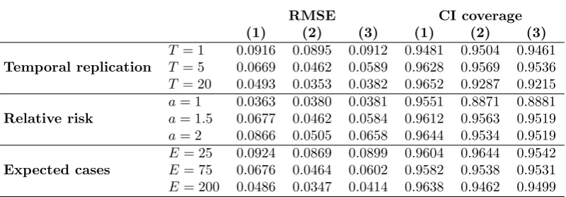
speci-Table 2. Median root mean-squared error (RMSE) and 95% credible interval coverages associated with the fitted risks for each model and each of the 9 simulation scenarios.

RMSE CI coverage

(1) (2) (3) (1) (2) (3)

Temporal replication

T = 1 0.0916 0.0895 0.0912 0.9481 0.9504 0.9461

T = 5 0.0669 0.0462 0.0589 0.9628 0.9569 0.9536

T = 20 0.0493 0.0353 0.0382 0.9652 0.9287 0.9215

Relative risk

a= 1 0.0363 0.0380 0.0381 0.9551 0.8871 0.8881

a= 1.5 0.0677 0.0462 0.0584 0.9612 0.9563 0.9519

a= 2 0.0866 0.0505 0.0658 0.9644 0.9534 0.9519

Expected cases

E= 25 0.0924 0.0869 0.0899 0.9604 0.9644 0.9542

E= 75 0.0676 0.0464 0.0602 0.9582 0.9538 0.9531

E= 200 0.0486 0.0347 0.0414 0.9638 0.9462 0.9499

ficity at identifying true step changes. These statistics were based on comparing E[wij|Y] to a threshold value p∗, where if E[wij|Y] < p∗ a step change was iden-tified where as for the converse no step change was declared. The value ofp∗ was varied from 0 to 1 at intervals of 0.01, and the ROC curve is a plot of sensitivity against specificity. However, for ease of presentation the Area Under the Curve (AUC) is presented here rather than the full ROC curve, and an AUC of one corre-sponds to perfect step change identification. We note that AUC was only computed for Models(2) and(3), as Model (1) has no mechanism for step change detection.

Table 2 shows the RMSE and credible interval coverages associated with each model across the nine simulation scenarios, from which a number of patterns emerge. Firstly, models(2)and(3)outperform the existing non-adaptive approach in terms of RMSE in all but thea= 1 scenario, in which no step changes exist and the RMSE values are hence similar. Model (2) outperforms model (3) in terms of RMSE in almost all cases, suggesting that the spatial smoothing imposed on the adjacency relationships w+ is sub-optimal compared with assuming each element wik ∈ w+

is a-priori independent. For all models RMSE decreases as both the number of

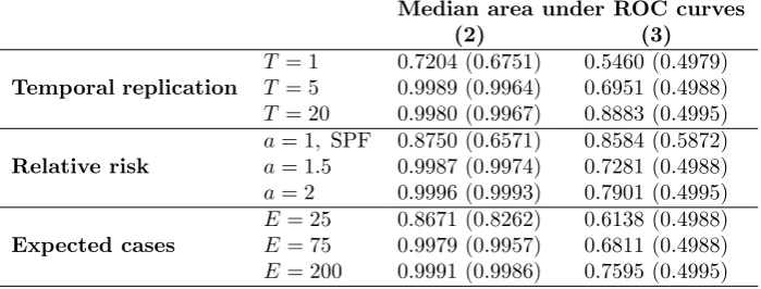
100 simulations for models(2)and(3). Bracketed figures correspond to the 10%

quantile of areas. Fora= 1 SPFdenotes the specificity since there are no true

step changes to identify in this scenario.

Median area under ROC curves

(2) (3)

Temporal replication

T = 1 0.7204 (0.6751) 0.5460 (0.4979)

T = 5 0.9989 (0.9964) 0.6951 (0.4988)

T = 20 0.9980 (0.9967) 0.8883 (0.4995)

Relative risk

a= 1, SPF 0.8750 (0.6571) 0.8584 (0.5872)

a= 1.5 0.9987 (0.9974) 0.7281 (0.4988)

a= 2 0.9996 (0.9993) 0.7901 (0.4995)

Expected cases

E= 25 0.8671 (0.8262) 0.6138 (0.4988)

E= 75 0.9979 (0.9957) 0.6811 (0.4988)

E= 200 0.9991 (0.9986) 0.7595 (0.4995)

Table 3 displays the median AUC statistic across the set of ROC curves calculated for the 100 simulated data sets from each scenario. The numbers in brackets are the tenth percentile of that distribution, and give a summary of the variation in the AUC statistics across the 100 simulated data sets. An exception to this is the

a = 1 scenario, which instead displays the specificity because as the risk surface is spatially smooth there are no true step changes to identify. For model (2) the median AUC values is close to the maximal value of 1, indicating very accurate step change identification. The exception to this occurs whenT = 1 which is when step change detection is based on only one realistaion of the spatial surface.

6. Results of the England case study

This section presents the results of the England circulatory and respiratory disease case study introduced in Section 2, where JSA is included as a covariate in all models. We apply two models to each data set, the global smoothing model of Rushworth et al. (2014) (Model(1)) and the adaptive smoothing model proposed here with the simplification that ρ = 0 (Model (2)). We do not apply the full adaptive model which estimates ρ because the simulation study showed it produced poorer results compared to Model (2). Inference for both models is based on 50,000 posterior samples, which are collected after a burn-in period of a further 50,000 samples. In analysing these data our goals are to: (i) estimate the spatio-temporal pattern in disease risk to quantify the extent of health inequalities; and (ii) estimate the location of any step changes in the unexplained spatial risk structure, which will assist in the identification of unmeasured confounders.

6.1. Model fit and risk estimation

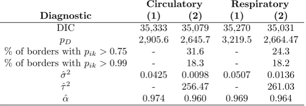
and respiratory admissions data sets.

Circulatory Respiratory

Diagnostic (1) (2) (1) (2)

DIC 35,333 35,079 35,270 35,031

pD 2,905.6 2,645.7 3,219.5 2,664.47

% of borders withpik>0.75 - 31.6 - 24.3

% of borders withpik>0.99 - 18.3 - 18.2

ˆ

σ2 0.0425 0.0098 0.0507 0.0136

ˆ

τ2 - 256.47 - 261.03

ˆ

α 0.974 0.960 0.969 0.964

between 0.96 and 0.98.

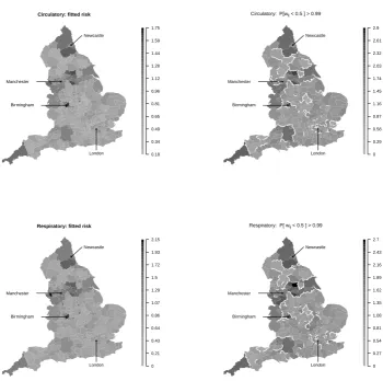
Maps of the average risks across all years from model(2) are displayed in the left column of Figure 4, and show similar spatial patterns in risk for both diseases, with a Pearson’s correlation coefficient of 0.948. The maps show that the average risk varies over space with values between (0.192, 1.634) and (0.176, 2.152) respectively for circulatory and respiratory disease, suggesting the presence of substantial health inequalities. These inequalities have generally widened over time, as the difference between highest and lowest respiratory disease risk was 1.78 in 2001 and 2.13 in 2010. For circulatory disease a similar pattern is evident, with an estimated difference between highest and lowest risk of 1.39 in 2001 and 1.54 in 2010.

6.2. Step change identification

England that incorporates Manchester and Yorkshire, even after adjusting for JSA. It is striking that these features are largely consistent between the two diseases, so that although the estimated risks have different overall magnitudes, they exhibit very similar spatial patterns. Public health professionals can use these results to identify potential risk factors for disease, by searching for risk factors that exhibit step changes in the same locations as those exhibited in Figure 4.

Circulatory: fitted risk

Newcastle Birmingham Manchester London 0.18 0.34 0.49 0.65 0.81 0.96 1.12 1.28 1.44 1.59 1.75

Circulatory: P[wij < 0.5 ] > 0.99

Newcastle Birmingham Manchester London 0 0.29 0.58 0.87 1.16 1.45 1.74 2.03 2.32 2.61 2.9

Respiratory: fitted risk

Newcastle Birmingham Manchester London 0 0.21 0.43 0.64 0.86 1.07 1.29 1.5 1.72 1.93 2.15

Respiratory: P[ wij < 0.5 ] > 0.99

Newcastle Birmingham Manchester London 0 0.27 0.54 0.81 1.08 1.35 1.62 1.89 2.16 2.43 2.7

Fig. 4. Maps showing the average risk surface (left column) and the unexplained compo-nent of the risk surface (right column) for both diseases. The top row relates to circulatory disease while the bottom row relates to respiratory disease. The white lines on the maps in the right column correspond to step changes that have been identified using a cutoff of

In this paper a new study of the spatio-temporal structure of circulatory and res-piratory disease risk in England is presented, with the goal of understanding the extent of health inequalities and whether the data present evidence of disparities in disease risk between pairs of adjacent regions. Consequently, a new spatially adap-tive smoothing model for disease risk was developed, that can estimate the location and strength of step-changes in disease risk. The model is a spatially adaptive ex-tension to the class of GMRF prior distributions, and is one of the first models for step change identification in spatio-temporal disease risk. Freely available software via theCARBayesST package forR is provided to allow others to apply our model to their own data, and this is one of the firstRpackages for spatio-temporal disease mapping.

The simulation study in Section 5 established the superiority of our model over existing global smoothing alternatives, in terms of both risk estimation and the quantification of uncertainty in disease risk. Our model was also successful at re-covering the locations of known step changes in simulated data, with AUC statistics close to one for a range of different scenarios. These AUC statistics were higher if the step changes were assumed to be independent in space, becausea-priori assum-ing spatial clusterassum-ing resulted in false step changes beassum-ing identified close to real step changes. Thus existing global smoothing models are sub-optimal for space time dis-ease mapping in two respects. Firstly, they smooth over such step changes leading to poorer estimation of disease risk, and secondly they cannot identify such step changes which themselves provides etiological evidence about potential unmeasured risk factors.

Section 6 described the application of the new model to the England hospital admis-sions data, from which strong evidence of step changes in the unexplained component of risk was found. Better model fit with a smaller number of effective parameters

achieved because increased levels of smoothing were possible in locations where step changes were not present. Thus existing models without this adaptive smoothing capability may overfit some data sets, by imposing too weak a spatial smoothing constraint due to the presence of step changes in risk. A striking association was found between the fitted risks and identified step changes between circulatory and respiratory disease, perhaps indicating the influence of the same unobserved risk factor (after allowing for socio-economic deprivation by JSA). Therefore in future work we will try and identify such unmeasured confounders, to see if the they are indeed common to both diseases.

Another avenue for future work is to use the model in an ecological regression con-text, where the effect of an exposure on disease risk is of primary interest rather than the spatio-temporal pattern in disease risk. The efficacy of adaptive smoothing models in this context may be to reduce spatial confounding between the random effects and the covariates as suggested by Clayton et al. (1993), and environmental factors such as air pollution would be a natural context for such work. A further avenue of future work is to consider spatio-temporal models for multiple diseases, such as circulatory and respiratory disease, simultaneously, thus allowing between disease correlations in step change locations to be utilised in the model.

8. Acknowledgements

This work was funded by the Engineering and Physical Sciences Research Council (EPSRC), via grant EP/J017442/1.

References

Anderson, C., D. Lee, and N. Dean (2014). Identifying clusters in bayesian disease mapping. Biostatistics 15, 457–469.

Bernardinelli, L., D. Clayton, C. Pascutto, C. Montomoli, M. Ghislandi, and M. Songini (1995). Bayesian analysis of spacetime variation in disease risk.

Besag, J., J. York, and A. Molli´e (1991). Bayesian image restoration, with two applications in spatial statistics. Annals of the Institute of Statistical Mathemat-ics 43(1), 1–20.

Brewer, M. J. and A. J. Nolan (2007). Variable smoothing in bayesian intrinsic autoregressions. Environmetrics 18(8), 841–857.

Brezger, A., L. Fahrmeir, and A. Hennerfeind (2007). Adaptive gaussian markov random fields with applications in human brain mapping. Journal of the Royal

Statistical Society: Series C (Applied Statistics) 56(3), 327–345.

Charras-Garrido, M., D. Abrial, J. De Go¨er, S. Dachian, and N. Peyrard (2012). Classification method for disease risk mapping based on discrete hidden markov random fields. Biostatistics 13(2), 241–255.

Clayton, D., L. Bernardinelli, and C. Montomoli (1993). Spatial Correlation in Ecological Analysis. Int J Epidemiol 22, 1193–1202, DOI:10.1093/ije/22.6.1193.

Green, P. J. and S. Richardson (2002). Hidden markov models and disease mapping.

Journal of the American statistical association 97(460), 1055–1070.

Knorr-Held, L. (2000). Bayesian modelling of inseparable space-time variation in disease risk. Statistics in Medicine 19(17-18), 2555–2567.

Lawson, A. B., J. Choi, B. Cai, M. Hossain, R. S. Kirby, and J. Liu (2012). Bayesian 2-stage space-time mixture modeling with spatial misalignment of the exposure in small area health data. Journal of agricultural, biological, and environmental statistics 17(3), 417–441.

Lee, D. and R. Mitchell (2013). Locally adaptive spatial smoothing using conditional auto-regressive models. Journal of the Royal Statistical Society: Series C (Applied Statistics) 62(4), 593–608.

Lee, D., A. Rushworth, and S. K. Sahu (2014). A bayesian localized conditional au-toregressive model for estimating the health effects of air pollution.Biometrics 70, 419–429.

Leroux, B., X. Lei, and N. Breslow (2000). Estimation of disease rates in small areas: A new mixed model for spatial dependence. In M. Halloran and D. Berry (Eds.),Statistical Models in Epidemiology, the Environment, and Clinical Trials, Volume 116 ofThe IMA Volumes in Mathematics and its Applications, pp. 179– 191. Springer New York.

Lu, H. and B. P. Carlin (2005). Bayesian areal wombling for geographical boundary analysis. Geographical Analysis 37(3), 265–285.

Lu, H., C. S. Reilly, S. Banerjee, and B. P. Carlin (2007). Bayesian areal wombling via adjacency modeling. Environmental and Ecological Statistics 14(4), 433–452.

Ma, H., B. P. Carlin, and S. Banerjee (2010). Hierarchical and joint site-edge meth-ods for medicare hospice service region boundary analysis. Biometrics 66(2), 355–364.

MacNab, Y. C. and C. Dean (2001). Autoregressive spatial smoothing and temporal spline smoothing for mapping rates. Biometrics 57(3), 949–956.

Office for National Statistics (2014). Inequality in healthly life expectancy at birth by national deciles of area deprivation: England, 2009-11.

Reich, B. J. and J. S. Hodges (2008). Modeling longitudinal spatial periodontal data: A spatially adaptive model with tools for specifying priors and checking fit.

Biometrics 64(3), 790–799.

Richardson, S., A. Thomson, N. Best, and P. Elliott (2004). Interpreting Poste-rior Relative Risk Estimates in Disease Mappling Studies. Environmental Health

Perspectives 112, 1016–1025.

Rue, H. and L. Held (2005). Gaussian Markov random fields: theory and

Rushworth, A., D. Lee, and R. Mitchell (2014). A spatio-temporal model for esti-mating the long-term effects of air pollution on respiratory hospital admissions in greater london. Spatial and Spatio-temporal Epidemiology.

Ugarte, M. D., T. Goicoa, and A. F. Militino (2010). Spatio-temporal modeling of mortality risks using penalized splines. Environmetrics 21(3-4), 270–289.

Wakefield, J. and A. Kim (2013). A bayesian model for cluster detection.

Biostatis-tics 14(4), 752–765.