MULTI-RADIO NETWORK OPTIMISATION USING BAYESIAN BELIEF PROPAGATION
Colin McGuire and Stephan Weiss
Centre for White Space Communications, Department of Electronic & Electrical Engineering
University of Strathclyde, Glasgow G1 1XW, Scotland
{
colin.mcguire,stephan.weiss
}
@strath.ac.uk
ABSTRACT
In this paper we show how 5 GHz and “TV White Space” wire-less networks can be combined to provide fixed access for a rural community. Using multiple technologies allows the advantages of each to be combined to overcome individual limitations when as-signing stations between networks. Specifically, we want to max-imise throughput under the constraint of satisfying both the desired individual station data rate and the transmit power within regula-tory limits. For this optimisation, we employ Pearl’s algorithm, a Bayesian belief propagation implementation, which is informed by statistics drawn from network trials on Isle of Tiree with 100 house-holds. The method confirms results obtained with an earlier deter-ministic approach.
Index Terms— heterogeneous networks; network optimisation; Bayesian belief propagation; white space communications; rural broadband access
1. INTRODUCTION
Rural broadband delivery through wireless links based on IEEE 802.11 [1] has been successfully used world-wide for rural access. Despite the wide channel bandwidths of IEEE 802.11 technologies in the GHz bands, its range can be limited due to the characteristics of the frequency bands used [2]. The “TV White Space” (TVWS) band is widely seen as a good candidate for long distances and non-LOS links [2, 3]; however, throughput can be limited by a small channel bandwidth.
Due to the modest power consumption of wireless networking equipment, previous demonstrations have powered equipment using renewable energy sources [1, 2]. Minimizing the power consump-tion also reduces the cost of a system making it economically viable. Therefore, this paper addresses the problem of optimising the power consumption in a rural two band (GHz/TVWS overlay) scenario, where stations can be assigned to either of the two networks. Us-ing multiple networks is regarded as a low cost solution to increase capacity [4], and offers the opportunity to reduce power consump-tion whilst maintaining quality of service [5, 6].
In [7] we showed how two radio access networks (RANs) oper-ating in TVWS and GHz bands can be combined to serve a commu-nity, where the assignment of stations between RANs changes based on network throughput requirements to minimize power consump-tion. In this paper, we update this model using statistical models of the networks obtained from analysis of a wireless rural broad-band network on the Scottish island of Tiree serving over 100 house-holds. By defining a probabilistic model of the network, we propose a scheme using Bayesian belief propagation network (BBN) [8] to determine the impact of assigning users to specific RANs in order to maximise the network data rate, while considering the overall power
consumption and heeding constraints on the transmit power due to regulatory restrictions.
Below, Sec. 2 discusses the probabilistic network model, which forms the basis of a BBN. With measurements and derivative quan-tities introduced in Sec. 3, Sec. 4 proposes the station assignment based on a BBN implementation using Pearl’s algorithm [9]. Simu-lations and results are provided in Sec. 5, with conclusions in Sec. 6.
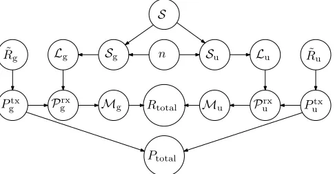
2. PROBABILISTIC NETWORK MODEL
The network consists ofNstations, were each station is described by a random variable representing the distance from the base station, forming a setS. The stations can be allocated to either network, described by the variablen. This creates a set of station distances on the GHz RAN,Sgand UHF RAN,Su.
The diagram in Fig. 1 relates the station assignment to an ex-pected minimum station data rateRtotal and power consumption
Ptotal. Each station distance inSa,a∈ {u,g}, has a corresponding
path loss,La. Given a minimum required data rate,R˜a for all sta-tions, this derives a required transmit powerPatx. The receive power
for each station in a networkParxcan be calculated using the trans-mit power and path loss for each station, resulting in a set of data rates for each stationMa. These data rates are used to calculate
the combined network throughput,Rtotal. The base station power consumptionPtotalis a function of the transmit powers, which,
to-gether with the combined data rateR, can be used to select a station assignmentn.
3. NODE DISTRIBUTION AND RELATIONSHIPS
The relationship betweenSa,La,Patx, ParxandMa is modelled
using a BBN shown in Fig. 2. Each node in the BBN represents a
S
n Su
Sg
Mg Rtotal
Ptotal
Mu Prx
u ˜
Rg Lg Lu
Ptx
u ˜
Ru
Ptx
g P
[image:1.595.318.561.579.705.2]rx g
P
txa
S
a,1S
a,2S
a,nL
a,2L
a,nL
a,1
P
rx
a
P
rxa
P
rxa
M
a,2M
a,nM
a,1.
.
.
.
.
.
.
.
.
Fig. 2. BBN describing dependencies of distance, path loss, receive power and data rate.
random variable with a belief, characterised by a probability den-sity function (PDF). Nodes are connected by conditional dependen-cies [8]. Conditional probability tables (CPTs) are used for each node to describe the relationship to its parents, which are upstream nodes in the directed graph. The CPTs are constructed using models of the relationships between nodes, described in the following sec-tions: distance between base station and consecutive nodes, distance and path loss, receive power given path loss and transmit power and data rate given receive power. Using Pearl’s algorithm [9], informa-tion across the graph is exchanged through nodes, by passing mes-sages. As the graph is acyclic, the beliefs will converge to a solute. The resultant beliefs of the data rates for each stationMacan then
be averaged to estimate the throughput of the network.
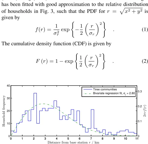
3.1. Household Distance Distribution
The majority of households are located close to the “hub” of the community, where a base station is typically situated. Fig. 3 shows the distribution of households from base stations in the Tiree com-munity broadband network.
A circularly symmetric normal distribution depending on x
(North) andy(West) coordinates with the base station at the origin has been fitted with good approximation to the relative distribution of households in Fig. 3, such that the PDF forr = px2+y2is given by
f(r) = 1
σ2
r
exp
(
−1 2
r σr
2)
. (1)
The cumulative density function (CDF) is given by
F(r) = 1−exp
(
1 2
r σr
2)
. (2)
0 1 2 3 4 5 6 7 8 9 10 11
0 10 20 30 40
Hou
se
h
ol
d
fr
eq
u
en
cy
Distance from base stationr/ km
0 1 2 3 4 5 6 7 8 9 10 110
0.1 0.2 0.3
2
π
r
f
(
r
)
Tiree communities Bivariate regression fit, σ
[image:2.595.56.299.75.177.2]r = 2.80
Fig. 3. Histogram of household distance from base station on Tiree.
S
a,1 Sa,2 Sa,n
Fig. 4. Probabilistic model of the multi-RAN network.
Fig. 3 shows the probability of finding a household between radiir
andr+drwithσr= 2.8km, which closely resembles the observed distribution.
The individual station distances, S, are described using an or-dered set ofN random variables where each variable has a PDF
f(r)and a CDFF(r)given by (1) and (2). The set is ordered from closest station to farthest station (1 → N), therefore the random variables representing each distance are conditionally dependent as shown in the graph in Fig. 4.
The PDF of stationkin the set ofNis given by
f(k)(r) =N f(r)
N−1
k−1
!
F(r)k−1(1−F(r))N−k . (3)
The joint PDFfi,j(u, v)of stationiat a distanceuand stationjat a distancev, where0≤i < j < Nandu < v, is given by
fi,j(u, v) = N!
(i−1)! (j−1−i)! (N−j)!f(u)f(v)F(u)
i−1
·(F(v)−F(u))j−1−i1−F(v)N−j . (4)
This allows the conditional PDF
fi|j(u, v) = fi,j(u, v)
fj(v) (5)
of stationsigivenjto be calculated. This conditional probability is used as the CPT linking consecutive station distance variables in the BBN.
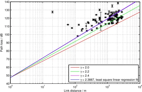
3.2. Propagation Model
The relationship between distance and path loss is describes using a simplified path-loss formula [2]. The average large-scale path lossL
between a transmitter and receiver in dB for a distancedin meters is given by
L=K+ 10γlog (d) , (6)
whereγ is the path loss exponent and K the reference path loss constant at a close-in distanced0. The latter depends on antenna characteristics and the average channel attenuation. This is obtained through field measurements or can be set to the free-space path gain at a referenced0in the antenna’s far field, which, assuming omni-directional antennas for an operating wavelengthλ, is given by
K= 20 log
λ
4πd0
. (7)
For this analysis, the values ofKandγwere determined through empirical analysis of the Tiree network, similar to [10] using re-ceived signal strength measurements recorded automatically on all links. A least squares linear regression fit was used to determine
γ given the measured K = 47.4 dBfor an operating frequency of5.6 GHz. Fig. 5 shows a scatter chart of calculated path losses for each station with error bars representing the standard deviation. Four path loss approximations are plotted with different path loss exponents ranging from the free space path loss withγ = 2.0to
[image:2.595.52.298.457.697.2]100 101 102 103 104 40
50 60 70 80 90 100 110 120 130 140
Link distance / m
Path loss / dB
γ = 2.0
γ = 2.2
γ = 2.4
[image:3.595.56.296.75.231.2]γ = 2.3887, least square linear regression fit
Fig. 5. Path lossLversus link distancedmeasured on Tiree, with linear approximations and a least squares fit.
3.3. Receiver Model
For a given transmission power and path loss, the receive power for stationson RANais given by
Ps,arx =P tx
a −Ls,a+Grx , (8)
assuming all quantities are measured in dB.
The possible modulation and coding scheme (MCS) rates for a set of stations in a RAN is denoted asMa. Each MCS rate has a
corresponding minimum receive power which is obtained through a lookup table. The set of minimum receive powers for all possible MCS levels is denoted asPmcs,rx. For each station receive power, the MCS rate used by stations,Ms,a, is determined by the range within whichPrx
s,afalls. The MCS receive powerPs,amcs,rx∈ Pmcs,rx
best suited for stationsis
Ps,amcs,rx= max
Pmcs,rx∈ Pmcs,rx|Pmcs,rx≤Ps,arx . (9)
3.4. Transmit Power Selection
The transmit powers ofA,Patx, depend on the assignmentN and
the path losses for stations inS and their association with either of the RANs. The crucial component is the GHz networkag, which must provide the transmission powerPgtxto support its associated
|Sg|stations.
To determinePgtx, we consider the minimum required transmit powerPstx,minto establish a connection with farthest stationson the
GHz RAN with the lowest data ratemcs = 0. The BBN in Fig. 2 is solved with nodePsrxset as evidence,Psrx=Psmcs=0,rx, and the
belief of nodePtxuninitialised. When the BBN converges, the mean of the belief ofPatxis taken as the transmit powerPstx,g required to associate stationswith the GHz RAN.
The transmit power for the UHF RAN,Ptx
u , is 30 dBm which is
a possible limit for TVWS transmissions recommended in the Cam-bridge TVWS Trial [11]. This is assumed to create a reliable con-nection for all stations.
3.5. Network Throughput Model
Given a set of MCS rates for each station on a RAN, the network throughput model calculates the expected user datagram proto-col (UDP) downlink data rate for each station using a model of the
IEEE 802.11 MAC layer in point coordination function (PCF) mode, which is described in [7].
With the expected data rate Ra in bits/s (bps) for each of the stations inSa,
Ra= LDATA
TPCF,a
, (10)
the minimum data rate for an individual station in the network,
Rtotal, is given by
Rtotal= min (Ra),∀a∈ A . (11)
In (10), LDATA is the length of the data packet in bits, which for
simplicity is assumed to be uniform across all stations to simulate a congested network. The total time required for a PCF exchange between the point coordinator and all associated stations is denoted asTPCFand therefore dependent on the data rate used by each station
Ma.
As beliefs of the MCS rates are available for each station, the mean values are used to estimate the network throughput. The net-work throughput for all pertinent combinations of station MCS rates is obtained using the model described above. Linear interpolation is performed on these combinations using the mean MCS rates to estimate the overall throughput.
3.6. Power Consumption Model
Based on lab measurements on the WindFi system [2] for both GHz and UHF radios, the power consumption of a radio is approximated by a function of the transmit powerPatx and transmit antenna gain Gtxfor each RAN described in [7]. The total power consumption of
the base stationPtotalis the sum of the power consumption of each
radio given coefficientsαa,βaandγa.
4. POWER-OPTIMISED STATION ASSIGNMENT
The stations are assigned to either of the two RANs to minimise the difference between the target data rateRtarget, which likely is time-varying, and the data rateR(Ni)provided by a specific station
assignment Ni = {Su,i,Sg,i} ∈ NAll with NAll the set of all
possible station assignments, NAll
=|S|+ 1. A data rateR(Ni)
below the target rate will penalise station users, while a higher rate utilises more transmit power than necessary. Therefore, optimising the assignmentNoptcan be formulated as a constrained optimisation problem
Nopt = arg min
Ni∈NAll
|Rtarget−R(Ni)| ,
s.t. R(Ni)≥Rtarget
Patx≤Pa,txmax,∀a∈ A , (12)
wherePa,txmaxis the maximum permissible transmission power. The transmit power will be minimised by keeping the data rate to a per-missible minimum in (12).
parameter value parameter value
γ 2.39 d0, σx 1 m, 2.8 km
LDATA 2312 bits fg, fu 5660 MHz, 630 MHz Ptx,max 30 dB αu, βu, γu 3.395e-07, 4.424, 2.555
Gtx, Grx 10 dB αg, βg, γg 2.292e-07, 4.381, 2.342 Pmcs,rx
g {−92,−89,−85,−85,−82,−78,−71,−68}dB
Pmcs,rx
[image:4.595.55.302.66.285.2]u {−103,−99,−98,−95,−89,−85,−78,−65}dB
Table 1. Simulation parameters based on measurements on Tiree.
0 1 2 3 4 5 6 7 8 9 10 11 12 13 14 15 16 17 18 19 20 0
5 10 15 20 25 30 35 40
Number of stations on GHz RAN
P
tx
/
d
B
m
[image:4.595.53.303.72.147.2]Transmit power to associate station on GHz RAN GHz transmit power limit
Fig. 6. Mean beliefs ofPtx
g with standard deviation after BBN
con-vergence to associate stations with the GHZ RAN.
5. MODELLING AND RESULTS
To solve the optimum station assignment problem in (12), we utilise a BBN using Pearl’s algorithm [9], and benchmark it against a previ-ous deterministic result that used an exhaustive search over a feasible set of assignments [7]. In the scenario, we assume that a base station servesN = 20stations, which is representative of the number of households served by three base stations on Tiree. Two networks are available for use:
• a UHF RAN atfu= 763MHz with 5 MHz bandwidth, or
• a GHz RAN atfg= 5.66GHz with 20 MHz bandwidth.
The parameters for both RANs are listed in Tab. 1 and are based on measurements taken on the Tiree network and WindFi parame-ters [2].
5.1. Impact of Station Assignment
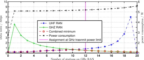
To determine the impact of station assignments, the BBN in Fig. 2 is used for the GHz network with the estimated transmit power re-quired for each possible assignment estimated in Fig 4 as discussed in Sec. 3.4. Fig. 6 plots the resulting mean transmit powers with stan-dard deviations after convergence. Re-running the BBN with these transmit powers as evidence ofPtxprovides estimates of individual station MCS rate beliefs within each RAN once converged. These are used to calculate the throughput using the model described in Sec. 3.5. Scaling the transmit power changes the assignmentn.
Fig. 7 shows the station data throughput for each RAN for all feasible sets of assignments which satisfy the constraint of a valid GHz RAN transmission power, Ptx
g ≤ Pmaxtx ; this excludes the eight stations furthest from the base station that cannot be served by the GHz RAN. The minimum combined station capacity increases from 0.20 Mbps when all stations are served by the UHF RAN to 0.67 Mbps in case stations are optimally assigned between RANs. Compared to [7] the greater path loss coefficient estimated for Tiree, reduces the number of stations which can be served with a legal transmit power. Scaling the transmit power only to associate stations at MCS rate 0 causes lower estimated throughputs.
0 2 4 6 8 10 12 14 16 18 20
0 1 2 3 4 5 6 7 8 9 10
Number of stations on GHz RAN
D
a
ta
ra
te
s
/
M
b
p
s
0 2 4 6 8 10 12 14 16 18 201
2 3 4 5 6
p
ow
er
co
n
su
m
p
ti
o
n
/
W
UHF RAN GHZ RAN Combined minimum Power consumption
[image:4.595.319.555.75.174.2]Assignment at GHz trasnmit power limit
Fig. 7. Individual station capacity on each RAN and base station power consumption given possible valid RAN assignments.
0 10 20 30 40 50 60 70 80
Hourly downstream bandwidth / Mbps
00:0001:0002:0003:0004:0005:0006:0007:0008:0009:0010:0011:0012:0013:0014:0015:0016:0017:0018:0019:0020:0021:0022:0023:0000:00
Average hourly bandwidth measurements Bandwidth utilisation fit
Fig. 8. Mean downlink bandwidth of Tiree network and fitted model.
As discussed in Sec. 4 the optimum station assignment can be viewed graphically from Fig. 7, where the case of optimum assign-ment is|Sopt,g|= 10. Given that the GHz RAN has four times the
bandwidth of the UHF RAN, intuitively the GHz RAN should serve as many users as the transmission power constraint allows. How-ever, in the optimum case only 50% of the stations are served by the GHz network. This is due to the better propagation characteristics of the UHF RAN, where stations are being served at a higher MCS rate compared to the GHz RAN.
5.2. GHz RAN Breathing to Minimize Power Consumption
To obtain realistic figures for the time-varying target rateRtarget that drives (12), we have used the downstream traffic model for the Tiree rural broadband network as a network utilisationu ∈ [0,1]
over a day. The Tiree broadband network allows the instantaneous bandwidth used on each link within the network to be monitored. Figure 8 shows the mean daily downstream bandwidth of traffic on the network internet backhaul, with standard deviations indicated by error bars. The relative large variance is do to the overall network consisting of only 100 stations. Using the averaged bandwidth mea-surements, a model of the hourly downstream bandwidth utilisation can be created by spline fitting. This models is overlaid onto the measurements in Fig. 8. A diurnal pattern is visible, were substan-tially less bandwidth is used during the night compared to day time. The target data rate for optimisation as discussed in Sec. 4 can be derived from this utilisation by normalising the optimum data rate for the assignment setN, such that
Rtarget=u·R(Nopt) . (13)
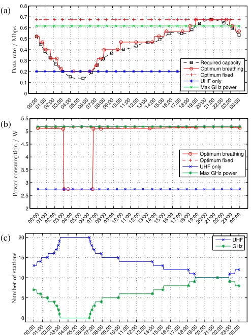
[image:4.595.56.297.167.279.2] [image:4.595.317.556.206.309.2](a)
0 0.1 0.2 0.3 0.4 0.5 0.6 0.7 0.8
00:0001:0002:0003:0004:0005:0006:0007:0008:0009:0010:0011:0012:0013:0014:0015:0016:0017:0018:0019:0020:0021:0022:0023:0000:00
D
at
a
rat
e
/
M
b
p
s
Required capacity Optimum breathing Optimum fixed UHF only Max GHz power
(b)
2 2.5 3 3.5 4 4.5 5 5.5
P
ow
er
con
su
m
p
ti
on
/
W
00:0001:0002:0003:0004:0005:0006:0007:0008:0009:0010:0011:0012:0013:0014:0015:0016:0017:0018:0019:0020:0021:0022:0023:0000:00
Optimum breathing Optimum fixed UHF only Max GHz power
(c)
0 5 10 15 20
N
u
m
b
er
of
st
at
ion
s
00:0001:0002:0003:0004:0005:0006:0007:0008:0009:0010:0011:0012:0013:0014:0015:0016:0017:0018:0019:0020:0021:0022:0023:0000:00
[image:5.595.54.301.72.402.2]UHF GHz
Fig. 9. Results of solving (12) in 15 min. intervals, showing (a) the required and offered capacity, (b) the total network power consump-tion and (c) the staconsump-tion assignment.
5.3. Benchmarks and Discussion
Fig. 9 (a) shows both the required and offered capacities for differ-ent dynamic and static assignmdiffer-ent schemes. In general, the data rate provided by the optimised scheme closely follows the target data rate above, thus satisfying the constraint and minimising transmis-sion power. Fig. 9 (b) compares the power consumption, where the optimised scheme exhibits a step up in power when the GHz RAN is required to satisfy the throughput demand during the peak time of the day. The fluctuating optimum station assignment is depicted in Fig. 9 (c).
For extreme assignments when only the UHF RAN is used, the power consumption of the network is minimised but cannot meet the capacity requirement during peak times from 07.00h to 03.00h. Maximising the size of the GHz RAN serves all GHz users at the highest MCS rate but requires the greatest power consumption. Due to the number of stations on the GHz RAN, the network capacity in this case is lower than with the optimum assignment.
Fig. 9 shows the case where the assignment is fixed to the max-imum throughput obtained from Fig. 7. The power consumption is constantly high even though the data rate is not required at all times. Dynamically changing the assignment, as proposed with the solution to (12), optimises the system at all times w.r.t. power consumption, providing a reduction of 7.3% compared to using the fixed assign-ment. A near-identical result is obtained with the deterministic ap-proach in [7], if both algorithms share the same parameters for Tiree.
6. CONCLUSION
This paper has proposed a probabilistic model for the station assign-ment in a fixed wireless rural access scenario, where stations can connect to a base station alternatively via GHz or TVWS RANs. The scenario used a Bayesian belief propagation network, imple-mented via Pearl’s algorithm, to optimised the capacity under mini-mum throughput and transmit power constraints based on parameter sets and distributions informed by a trial on Tiree.
The results agree with an earlier deterministic approach, which had been adjusted for a smaller trial on a second island — the Isle of Bute in Scotland — when using the Tiree parameters. In partic-ular the station assignment at the edge of the two networks is inter-esting, where the lower-bandwidth TVWS network is favoured over the GHz one by opting for a higher MCS rate to exploit the enhanced propagation characteristics that the TVWS band enjoys.
The Bayesian belief propagation approach has two distinct ad-vantages. Firstly, Pearl’s algorithm is guaranteed to converge for non-loopy graphs as used here, enhancing the requirement of an ex-haustive search in the deterministic method. Secondly, the modelling of uncertainty and insertion of evidence, where available, can signif-icantly enhance the accuracy and applicability of this approach.
REFERENCES
[1] G. Bernardi, P. Buneman, and M.K. Marina, “Tegola tiered mesh network testbed in rural scotland,” inACM Workshop Wirel. Netw. & Sys. Developing Regions, NY, pp. 9–16, 2008. [2] C. McGuire, M.R. Brew, F. Darbari, G. Bolton, A.
McMa-hon, D.H. Crawford, Stephan Weiss, and Robert Stewart, “HopScotch — a low-power green base station network for rural broadband access,” EURASIP J. Wirel. Comms & Netw.,112:1–12, 2012.
[3] Y.-C. Liang, A.T, Hoang, and H.-H. Chen, “Cognitive radio on TV bands: a new approach to provide wireless connectivity for rural areas,”IEEE Wirel. Comms,15(3): 16–22, June 2008. [4] S.P. Yeh, S. Talwar, G. Wu, N. Himayat, and K. Johnsson, “Capacity and coverage enhancement in heterogeneous net-works,”IEEE Wirel. Comms,18(3): 32–38, June 2011. [5] T.Q.S. Quek, W.C. Cheung, and M. Kountouris, “Energy
effi-ciency analysis of two-tier heterogeneous networks,” in11th Eur. Wirel. Conf., April 2011.
[6] Y. Hou, and D.I. Laurenson, “Energy efficiency of high QoS heterogeneous wireless communication network,” inIEEE 72nd Vehicular Tech. Conf., pp. 1–5, Sept 2010.
[7] C. McGuire and S. Weiss, “Power-optimised multi-radio net-work under varying throughput constraints for rural broadband access,” inEUSIPCO, 2013.
[8] H.A. Loeliger, “An introduction to factor graphs,” IEEE Sig. Proc. Mag.,21(1): 28–41, 2004.
[9] R.J. McEliece, D.J.C. Mackay and J. Cheng, “Turbo decoding as an instance of Pearls belief propagation algorithm,” IEEE J. Sel. Areas Comms,16(2): 140–152, 1998.
[10] V.S. Abhayawardhana, I.J. Wassell, D. Crosby, M.P. Sellars, and M.G. Brown, “Comparison of empirical propagation path loss models for fixed wireless access systems,” inIEEE 61st Vehicular Tech. Conf., pp. 73–77, May 2005.