LIDAR-based Wind Speed Modelling and
Control System Design
Mengling Wang, Hong Yue, Jie Bao, William. E. Leithead
Department of Electronic and Electrical Engineering University of Strathclyde, Glasgow, United KingdomE-mails: [email protected]; [email protected]; [email protected]; [email protected]
Abstract—The main objective of this work is to explore the feasibility of using LIght Detection And Ranging (LIDAR) measurement and develop feedforward control strategy to improve wind turbine operation.Firstly the Pseudo LIDAR measurement data is produced using software package GH Bladed across a distance from the turbine to the wind measurement points. Next the transfer function representing the evolution of wind speed is developed. Based on this wind evolution model, a model-inverse feedforward control strategy is employed for the pitch control at above-rated wind conditions, in which LIDAR measured wind speed is fed into the feedforward. Finally the baseline feedback controller is augmented by the developed feedforward control. This control system is developed based on a Supergen 5MW wind turbine model linearised at the operating point, but tested with the nonlinear model of the same system. The system performances with and without the feedforward control channel are compared. Simulation results suggest that with LIDAR information, the added feedforward control has the potential to reduce blade and tower loads in comparison to a baseline feedback control alone.
Keywords- wind turbine control; LIght Detection And Ranging (LIDAR); disturbance rejection; feedforward control; wind speed evolution
I. INTRODUCTION
Advanced control is one of many options that can contribute to improved performance and decreased cost of wind energy production. High performance and reliable controllers could increase efficiency of power generation and reduce cost of operation and maintenance [1, 2]. In recent years, motivated by higher expectation of wind turbine performance, increased attention has been paid to new measurement technologies, among which LIDAR (LIght Detection And Ranging) is able to provide the measurement of the wind upstream of the wind turbine and preview disturbance information. In the past decade, a number of wind turbine control strategies have been proposed, in which wind speed measurement are either provided or potentially provided by LIDAR.
During operation of wind measurement, a LIDAR emits a laser beam to the target wind field, and this laser beam is then backscattered by the small aerosols and particles in the wind field and then received by the LIDAR detector. The wind speed can therefore be calculated by employing the Doppler frequency shift between the two beams and the wavelength of the laser beams. With the help of preview wind measurement, feedforward control strategy is introduced into wind
turbine operations to reduce wind turbine structural loads [3, 4]. In some recent work, a feedforward channel is added to the baseline feedback control system. In this case, the feedforward controller can be designed independently of the feedback controller and will not affect the closed-loop stability. In [3], real LIDAR wind measurements information is used in wind turbine control systems instead of using an effective wind speed, where the results show reduction of tower and blade fatigue loads at high turbulent wind speeds. In [5], two feedforward controllers were designed to combine with two baseline feedback controllers, one applying model-inverse feedforward control for collective pitch control, and the other applying a shaped compensator for individual pitch control. Both of them enabled wind speed measurements that could be potentially provided by LIDAR as inputs to the feedforward controllers. An adaptive feedforward controller was proposed based on filtered-x recursive least algorithm [6].
Model predictive control (MPC) has proved to be an effective tool for multivariable constrained control systems, such as wind turbines. Henriksen et al. present the nonlinear MPC algorithm using future wind speeds in the prediction horizon [7]. In [8], an approach is proposed to deal with optimization problem of MPC. The nonlinear wind turbine model is linearised at different operating points, which are determined by the effective wind speed on the rotor disc. LIDAR wind speed measurement is used as a scheduling parameter.
While most of the research work concentrates on testing the load reduction performance by introducing LIDAR wind speed measurements, the energy capture performance of LIDAR-based control in below rated conditions was also investigated [9]. However, their results suggest that LIDAR-based control has limited improvements on energy capture. Therefore, applying LIDAR measurements in above rated pitch control could be more beneficial. The feasibility of applying LIDAR into wind turbine control systems needs further investigation. This motivates the work in the present paper. In this work, a wind evolution model is initially developed using the pseudo-LIDAR measurement data produced by Bladed, based on which a feedforward controller is designed and integrated to a baseline feedback controller.
The rest of the paper is organised as follows. In Section II, the details about the feedforward controller design are introduced. The wind speed evolution model is developed in Section III. Simulation studies are
conducted using an industrial-scale wind turbine model and the results are discussed in Section IV. The conclusions are summarized in Section V.
II. FEEDFORWARD CONTROLLER DESIGN
A. Feedback Baseline Controller
[image:2.595.320.513.253.447.2]A standard baseline wind turbine controller normally consists of two parts. One is the torque controller which accounts for below rated operation, and the other is the pitch controller which accounts for above rated operation. In below rated conditions, torque demand is employed to ensure the tracking of the maximum power coefficient so that the maximum energy capture is achieved. In above rated conditions, pitch demand is employed to assure the generated power being maintained not to exceed its rated value, see [10] and [11]. The conventional feedback pitch control diagram is shown in Fig. 1, which is taken as the baseline controller.
Figure 1. Block diagram of baseline feedback wind turbine control
B. Feedforward Controller
[image:2.595.63.285.290.385.2]LIDAR is able to provide preview information of wind disturbances at various distances in front of wind turbines. This feature can be used in feedforward control to improve disturbance rejection. This research augments the feedback pitch controller with a feedforward control term (see Fig. 2) to alleviate turbine loads in above rated wind speed conditions. Fig.2 shows a model-inverse-based strategy for designing feedforward controllers. The linear model-inverse feedforward controller is used to cancel the effect from the turbulence in wind speed on the wind turbine generator speed.
Figure 2. Combined feedback and feedforward control
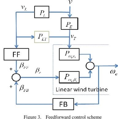
Based on Fig. 1 and Fig. 2, a feedforward control scheme is developed and shown in Fig. 3. The primary control goal of the whole control system is to maintain the actual greater speed 𝜔𝑔_𝑎𝑐𝑡𝑢𝑎𝑙 at rated generator speed value 𝜔𝑔_𝑟𝑎𝑡𝑒𝑑 in the presence of varying wind 𝑣 at above
rated conditions by adjusting the total pitch angle command 𝛽𝑐. 𝑣𝑇 is the turbine wind speed, which
indicates the wind speed approaching the turbine blades.
𝑣 evolves to 𝑣𝑇 on its way to the turbine and its variation
disturbs the wind turbine system. The block 𝑃𝐸 represents
this evolution. The measurement of wind speed by a LIDAR sensor is 𝑣𝐿(line of sight wind speed). 𝑃𝐿 is the
LIDAR system transferring 𝑣 to 𝑣𝐿.𝐹𝐵 is the feedback
controller and 𝐹𝐹 is the feedforward controller. The linear wind turbine model includes subsystems 𝑃𝜔𝑒𝛽𝑐 and
𝑃𝜔𝑒𝑣𝑡. 𝑃𝜔𝑒𝛽𝑐 maps collective blade pitch error 𝛽 to
generator speed error 𝜔𝑒 (𝜔𝑔_𝑎𝑐𝑡𝑢𝑎𝑙− 𝜔𝑔_𝑟𝑎𝑡𝑒𝑑) and
𝑃𝜔𝑒𝑣𝑡 maps 𝑣𝑇 to 𝜔𝑒. The output of feedforward
controller 𝛽𝐹𝐹 is added to the feedback pitch angle 𝛽𝐹𝐵 of collective pitch feedback controller.
Figure 3. Feedforward control scheme
Following the control strategy in Fig. 3, we have
𝜔𝑒= (𝑣 ∙ 𝑃𝐿∙ 𝐹𝐹 + ω𝑒∙ 𝐹𝐵) ∙ 𝑃𝜔𝑒𝛽𝑐+ 𝜈 ∙ 𝑃𝐸∙ 𝑃𝜔𝑒𝑣𝑡 (1)
Since it is expected that the tracking error of generator speed should be zero, i.e., 𝜔𝑒= 0 [6],
𝑣 ∙ 𝑃𝐿∙ 𝑃𝜔𝑒𝛽𝑐∙ 𝐹𝐹 = −𝜈 ∙ 𝑃𝐸∙ 𝑃𝜔𝑒𝑣𝑡 (2)
The feedforward controller is solved as
𝐹𝐹 = −𝑃𝜔𝑒𝛽𝑐
−1∙ 𝑃
𝜔𝑒𝑣𝑡 ∙ 𝑃𝐸∙ 𝑃𝐿
−1
(3)
where 𝑃𝜔𝑒𝛽𝑐−1 and 𝑃𝜔𝑒𝑣𝑡 can be obtained from turbine
modelling, but wind evolution 𝑃𝐸 and LIDAR system 𝑃𝐿
are very complex and difficult to model. In this research, the transfer function between 𝑣𝐿 and 𝑣𝑇, which is
PE∙ PL−1 is approximated by a transfer function
𝑃𝐿𝑇(𝑠) = 𝑆 𝑆𝐿𝑇(𝑠)
𝐿𝐿(𝑠) (4)
where S𝐿𝑇 is the cross spectrum between the LIDAR
measurements and the turbine wind speed, S𝐿𝐿 is the auto spectrum of the LIDAR measurements across the distance from the measurement point to wind turbine blades.
The feedforward controller is then written as
𝐹𝐹 = −𝑃𝜔𝑒𝛽𝑐
−1∙ 𝑃
[image:2.595.63.283.557.684.2]It is remarkable that the non-minimum phase zeros contained in 𝑃𝜔𝑒𝛽𝑐 would become poles that cause the
system to be unstable after inversing. Therefore, a stable approximation should be used instead of the exact inverse of 𝑃𝜔𝑒𝛽𝑐. Related work will be introduced later.
In the next section, the evolution of LIDAR measurements across the distance from the measurement point to wind turbine blades is developed. The cross spectrum between turbine wind speed and LIDAR measurements and the auto spectrum of LIDAR measurements are calculated.
III. WIND SPEED EVOLUTION MODELLING
A. LIDAR Wind Speed Simulation
[image:3.595.62.282.337.478.2]According to the feedforward control loop in Fig. 3, LIDAR measured wind speed is fed into the feedforward controller. In this work, the simulated LIDAR measurements are used in modelling. Taylor’s frozen turbulence hypothesis is employed, which assumes that the turbulent wind field is unaffected when approaching the turbine and moving with average wind speed.
Figure 4. 3D wind volume simulated by Bladed
[image:3.595.316.529.352.455.2]The continuous LIDAR shoots a continuous beam of light to the atmosphere and again all particles in the atmosphere, along the light of signal of the beam will reflect some of this light. These systems use the same frequency shift in the reflection, to determine the velocity of the particles. Each wind measurement is a vector with components at different directions. Here, only the component of the wind vector in laser beam direction (line of sight) wind speed is detected. It is constructed by averaging over the circular trajectory [12].
TABLE I. CHARACTERISES OF 3D TURBULENCE
Bladed uses a 3-dimensional turbulent wind field with defined spectral and spatial covariance characteristics to represent real atmospheric turbulence. This option will give the most realistic predictions of loads and performance in normal conditions. In Bladed, wind speed is displayed as a vector of 3 components: Longitudinal component x(t), Lateral component y(t) and Vertical component z(t), see Fig. 4. The parameters set up for the wind field simulation are listed in Table I. In this work, rectangular scan circle is used instead of round circle.
According to the scan principle of LIDAR instrument and Bladed display of wind field in Fig. 4, 𝑣𝑇(𝑡𝑇, 𝑥𝑇) and
𝑣𝐿𝑖(𝑡𝐿𝑖, 𝑥𝐿𝑖)(𝑖 = 1, ⋯ ,6) are points sampled from Bladed.
Wind field in the x direction to represent the turbine wind speed and LIDAR measurements. 𝑣𝑇(𝑥𝑇 = 0𝑚) is
assumed as the turbine wind speed, which is the mean wind fluctuation over the turbine plane. 𝑣𝐿𝑖(𝑡𝐿𝑖, 𝑥𝐿𝑖)(𝑖 =
1, ⋯ ,6) are assumed as LIDAR measurements with preview distances of 30m, 60m, 90m, 120m, 160m and 190m respectively (𝑥𝐿1= 30𝑚, 𝑥𝐿2= 60𝑚, 𝑥𝐿3=
90𝑚, 𝑥𝐿4= 120𝑚, 𝑥𝐿5= 160𝑚, 𝑥𝐿6= 190𝑚). Each
[image:3.595.308.526.553.723.2]wind speed is the mean wind fluctuation over an area lying in the y-z plane. The distribution of all wind speed points is shown in Fig. 5.
Figure 5. Distribution of the turbine wind speed and LIDAR measurements
In Fig. 5, the wind speed evolves in the direction of distance x. There is no cross correlation between
𝑣𝑇(𝑡𝑇, 𝑥𝑇) and 𝑣𝐿𝑖(𝑡𝐿𝑖, 𝑥𝐿𝑖)(𝑖 = 1, ⋯ ,6). Therefore, the
strategy of sampling points in the wind field is needed to be modified.
Figure 6. Schematics of wind speed sampling in Bladed Turbulence length
scales
Component of turbulence
Longitudinal Lateral Vertical
Along x m 244.671 58.8681 21.1883
Along y m 79.6605 76.6657 13.7971
Along z m 59.2508 28.5117 20.5243
Turbulence
[image:3.595.51.273.626.749.2]As the Bladed wind field is frozen and isotropic, the variation of the wind speed fluctuation in the x direction at a point can be equally represented by the component in the y direction as well as the component in the z direction. Hence, as depicted in Fig. 6, the cross correlation between the mean wind speed fluctuations over two areas displaced by a distance d in the x direction can be estimated from the areas lying in x-y planes separated by a distance of d in the y direction and the fluctuations in the z direction. Time evolution can be represented by moving the plates through the wind field in the z direction. Hence, the distribution of turbine wind speed and LIDAR measurements can be modified from Fig. 5 to Fig. 7. 𝑣𝑇(𝑡𝑇, 𝑥𝑇) and 𝑣𝐿𝑖(𝑡𝐿𝑖, 𝑥𝐿𝑖)(𝑖 = 1, ⋯ ,6) represent
[image:4.595.310.531.284.409.2]mean wind fluctuations in x-y plane, with time evolution in the z direction.
Figure 7. Modified distribution of the turbine wind speed and LIDAR measurements
[image:4.595.63.293.414.564.2]B. Cross Spectrum of Wind Speed
Figure 8. Cross spectrum of the turbine wind speed and LIDAR measurements
Figure 9. Auto spectrum of LIDAR measurements
Fig. 8 shows the cross spectrum of the turbine wind speed
vT and LIDAR measurements. The auto spectrum of
vLi(tLi, xLi)(i = 1, ⋯ ,6) can be seen in Fig. 9.
C. Transfer Function
Following the results of cross spectrum 𝑆𝐿𝑇 and auto
spectrum 𝑆𝐿𝐿, the transfer function 𝑃𝐿𝑇 in equation (4) is approximated by a first order low-pass filter using system identification method, see [13] for details.
𝑃𝐿𝑇(𝑠) = −8.102×10
−7
𝑠+0.02831 (6)
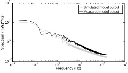
The transfer function model 𝑃𝐿𝑇 has been validated
against cross spectrum 𝑆(𝑣𝑡, 𝑣𝐿1), see Fig. 10. It can be
seen that the shapes of the simulated model output and the measured model output match reasonably well. Therefore, the transfer function is acceptable for the controller design.
Figure 10. Comparison of model output from (5) and ‘measured’ model output
IV. SIMULATION STUDY
In this work, the simulation study is implemented using the Supergen 5MW exemplar wind turbine model developed in the University of Strathclyde. This is a non-linear model that is constructed in Simulink. It contains 3 main parts, the pitch mechanism, the aero-rotor and the drive train model. The main turbine parameters are listed in Table II. More details can be found in [9, 14]. A matched 5 MW Supergen feedback controller is used here as the baseline controller.
TABLE II. WIND TURBINE PARAMETERS [14]
Turbine parameters
Rotor radius [m] 63
Effective blade length [m] 45
Hub height [m] 90
Maximum generator speed in
generation mode [rad/s] 120
Cut in wind speed [m/s] 4
Cut out wind speed [m/s] 25
Nominal generator torque [Nm] 46372.7
Air density [kg/m^3] 1.225
Gearbox ratio 97
Considering one input and output in each case, the nonlinear wind turbine model can be linearised at the
10-2 10-1 100 101 102 103
10-10 10-8 10-6 10-4 10-2 100 102
Frequency (Hz)
Cr
os
s
S
pe
c
tr
um
(
(m
/s
)
2/Hz
)
S(vt,vl1) S(vt,vl2) S(vt,vl3) S(vt,vl4) S(vt,vl5) S(vt,vl6)
10-2 10-1 100 101 102 103
10-6 10-4 10-2 100 102 104
Frequency (Hz)
S
pe
c
tr
um
(
(m
/s
)
2/Hz
)
vl1 vl2 vl3 vl4 vl5 vl6
10-2 10-1 100 101 102 103
10-10
10-5
100
105
Frequency (Hz)
S
pe
c
tr
um
(
(m
/s
)
2/Hz
)
[image:4.595.72.299.599.738.2]operating point, and a 1inearised state-space model is then produced involving 11 state variables. This state-space model can be further written as a continuous transfer function model. The simulation in this work is conducted at 16m/s mean wind speed and the wind speed fluctuation are modeled by a set of small steps added to the mean wind speed. The transfer functions, 𝑃𝜔𝑒𝛽𝑐 and
𝑃𝜔𝑒𝑣𝑡 are obtained by discretization of the two continuous
transfer function models, respectively, with a sampling rate of 0.0125s.
The transfer function between the generator speed error to the pitch demand is developed
𝑃𝜔𝑒𝛽𝑐(𝑧) =𝑊𝐵(𝑧)
1(𝑧) (7)
in which
𝐵(𝑧) = −1.1095(𝑧2− 1.9998𝑧 + 0.902)
(𝑧2− 2.0502𝑧 + 1.0546)
(𝑧2− 2𝑧 + 1.0005)(𝑧2− 1.9996𝑧 + 1)
(z + 1.1532) (z − 0.2523) (1)
𝑊1(𝑧) = (𝑧2+ 0.3156𝑧 + 0.624)
(𝑧2− 1.9796𝑧 + 0.9922)
(𝑧2− 1.9528𝑧 + 0.9570)
(𝑧2− 2.0022𝑧 + 0.9937)
(𝑧2− 1.9918𝑧 + 1.0067)
(𝑧 − 0.9942)
(2)
The transfer function between the generator speed error to the approaching blade wind speed is written as
𝑃𝜔𝑒𝑣𝑡(𝑧) =𝑊𝑉(𝑧)
2(𝑧) (8)
with
𝑉(𝑧) = (2.5921 × 10⁻⁵)(𝑧2− 1.9948𝑧 + 1.0004)
(𝑧2− 1.9992𝑧 + 0.9997)
(𝑧2− 1.9992𝑧 + 0.9997)
(z + 9.1961)(z + 1.0895)(z − 0.2666) (z + 0.1549)
(1)
𝑊2(𝑧) = (𝑧2+ 0.3156𝑧 + 0.624)
(𝑧2− 1.9796𝑧 + 0.9921)
(𝑧2− 1.9528𝑧 + 0.9562)
(𝑧2− 2.0022𝑧 + 1.0028)
(𝑧2− 1.9918𝑧 + 0.9923)
(𝑧 − 1.0002)
(2)
The feedforward controller is obtained from (5) that gives
𝐹𝐹(𝑧) = −𝑊1(𝑧)𝑉(𝑧) 𝑃𝐿𝑇
𝐵(𝑧)𝑊2(𝑧) (9)
It can be seen that the developed feedforward controller is of a high order which is inconvenient for tuning. This model is therefore firstly reduced by non-minimum phase zeros ignore (NPZ-Ignore) technique to remove non-minimum phase zeros, and further reduced to 3rd-order controller as shown in (10) via approximation fitting [15]. In order to fine tune the reduced-order controller, a tuning factor, 𝑘𝐹𝐹, is introduced in the
transfer function of 𝐹𝐹. This tuning function can also address modelling uncertainty to some extent. In this work, the designed value for 𝑘𝐹𝐹 is 2.336 × 10⁻⁵ to start
with. The fine-tuned setting is 𝑘𝐹𝐹 = 2 × 10⁻⁴,
𝐹𝐹(𝑧) = 𝑘𝐹𝐹×(𝑧+9.1961)(𝑧−0.2666)(𝑧+0.1549)𝑧3 (10)
Figure 11. Comparison of the pitch angle before and after the addtion of the feedforward controller
As shown in Fig. 11, with the feedforward controller, a decrease in the pitch angle demand power spectral density (PSD) is achieved. The decrease not only saves the driving energy but also helps to expand lifetime of pitch actuators.
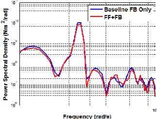
Figure 12. Comparison of the tower acceleration before and after the addtion of the feedforward controller
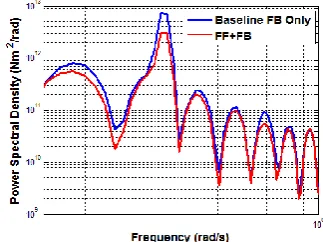
Figure 13. Comparison of the out-of-plane rotor torque before and after the addtion of the feedforward controller
[image:5.595.327.532.74.245.2] [image:5.595.337.498.347.467.2] [image:5.595.335.497.509.630.2]Figure 14. Comparison of the generator power before and after the addtion of the feedfoward controller
The comparison is also made for the generated power, as shown in Fig. 14. It can be seen that with or without the feedforward control channel, there is no clear difference between the power generated. This indicates that by introducing the feedforward controller for disturbance rejection, the power generation performance can still be maintained.
V. CONCLUSIONS
In this paper, the control strategy for designing LIDAR-based feedforward controllers has been presented. A model-inversed feedforward pitch controller is combined with the baseline feedback pitch controller of the Supergen 5MW wind turbine model.
The LIDAR measurements and the turbine wind speed are simulated by Bladed. The cross spectrum between them and the auto spectrum of LIDAR wind speed measurements are studied. The results are used to develop the transfer function representing the evolution of LIDAR measurements across the distance from the measurement point to the wind turbine blades. At last, the feedforward controller is designed based on the Supergen linear wind turbine model and the transfer function.
The performance of the feedfoward controller is evaluated at wind speed 16m/s. The Simulink simulation study shows that the feedforward/feedback controller has achieved improved performance on reducing the fluctuations of the pitch angle demand, tower acceleration and the out-of-plane torque of the rotor without degrading the energy capture seriously. It should be noted that in above-rated operating conditions, the main function of the baseline feedback pitch control is to maintain the generated power at rated power level. For large scale wind turbines, load reduction is another crucial control target, which can be handled by introducing extra feedback loops and/or feedforward channels. In our work, we consider a feedforward controller mainly to take advantages of the more comprehensive LIDAR measurement information, which should help to reduce the effects of disturbance brought by the wind speed uncertainty. In fact, the feedforward controller design can be regarded as independent of the feedback controller design, which means the feedback control performance won’t be deteriorated by the feedforward channel.
In our future work, the performance of feedforward controller and other LIDAR-based control strategies will be evaluated by calculating Damage Equivalent Loads (DEL), which can give more apparent comparisons between different control options in load reduction of large-scale wind turbine systems.
REFERENCES
[1] T. Burton, D. Sharpe, N. Jenkins, and E. Bossanyi, Wind energy handbook: John Wiley & Sons, 2001.
[2] F. D. Bianchi, H. De Battista, and R. J. Mantz, Wind turbine control systems: principles, modelling and gain scheduling design: Springer Science & Business Media, 2006.
[3] D. Schlipf, D. J. Schlipf, and M. Kühn, "Nonlinear model predictive control of wind turbines using LIDAR," Wind Energy, vol. 16, pp. 1107-1129, 2013.
[4] D. Schlipf, P. Fleming, F. Haizmann, A. Scholbrock, M. Hofsäß, A. Wright, et al., "Field testing of feedforward collective pitch control on the CART2 using a nacelle-based lidar scanner," in the Proceedings of The Science of Making Torque from Wind 2012, Oldenburg, Germany
[5] L. Y. Pao, F Dunne, A. D. Wright, B Jonkman, N Kelley and E Simley, "Adding feedforward blade pitch control for load mitigation in wind turbines non-causal series expansion, preview control, and optimized FIR filter methods," Technical Report, University of Colorado, Boulder, CO, USA 2011.
[6] L. C. Henriksen, N. K. Poulsen, and M. H. Hansen, "Nonlinear model predictive control of a simplified wind turbine," in 18th World Congress of the International Federation of Automatic Control, 2011, pp. 551-556.
[7] M. Mirzaei, M. Soltani, N. K. Poulsen, and H. H. Niemann, "An MPC approach to individual pitch control of wind turbines using uncertain LIDAR measurements," in 2013 European Control Conference (ECC), Zurich, Switzerland, 2013, pp. 490-495.
[8] N. Wang, "LIDAR-assisted feedforward and feedback control design for wind turbine tower load mitigation and power capture enhancement," PhD Thesis, Colorado School of Mines, 2013.
[9] W. E. Leithead and B. Connor, "Control of variable speed wind turbines: dynamic models," International Journal of Control, vol. 73, pp. 1173-1188, 2000.
[10] A. P. Chatzopoulos, "Full envelope wind turbine controller design for power regulation and tower load reduction," PhD Thesis, University of Strathclyde, 2011.
[11] N. Wang, K. E. Johnson, and A. D. Wright, "FX-RLS-based feedforward control for LIDAR-enabled wind turbine load mitigation," Control Systems Technology, IEEE Transactions on, vol. 20, pp. 1212-1222, 2012.
[12] D. Schlipf, "LIDAR assisted collective pitch control," Technical Report, University of Stuttgart, 2011.
[13] M. Wang, "Feedforward wind turbine controller design using LIDAR," Master Thesis , University of Strathclyde, April, 2015.
[14] A. Stock, "Guide to the Supergen controllers," Technical Report, University of Strathclyde, 2014
[image:6.595.86.248.80.203.2]