The Relative Efficiency of Automatic and Discretionary Industrial Aid

S

TRATHCLYDE

D

P

E

The Relative Efficiency of Automatic and Discretionary

Industrial Aid

B

J. Kim Swales

N

.

08-12

D

E

U

S

The Relative Efficiency of Automatic and Discretionary Industrial Aid*

J. Kim Swales

Fraser of Allander Institute, Department of Economics, University of Strathclyde and Centre for Public Policy for Regions, Universities of Glasgow and Strathclyde.

Abstract

1. Introduction

For the last two decades, the primary instruments for UK regional policy have been discretionary subsidies. In particular, in 1988 the discretionary Regional Selective Assistance (RSA) replaced the automatic Regional Development Grant (RDG) as the main systematic aid for industrial regeneration.i For a particular project, the receipt of an automatic subsidy depends on that project’s meeting a clear set of easily verified conditions. However, a discretionary subsidy is allocated on project criteria that are initially private information to the firm.

Two general aspects of discretionary subsidies that certainly apply to RSA are the following. First, the subsidy is targeted at “additional” projects: projects that would not have been implemented without the subsidy. Second, the subsidy given to additional projects is calculated as the minimum necessary for the project to proceed (HM Treasury, 2003; Scottish Executive, 2006). In this respect, discretionary subsidies are thought to be more efficient than automatic subsidies, where many of the aided projects are non-additional and all projects receive the same subsidy rate.

However, the use of discretionary subsidies raises three fundamental difficulties. First, discretionary subsidies have potentially higher administration costs, stemming from the need for the government to appraise in detail each project individually. Second, the government is likely to make appraisal errors, which reduces the effectiveness of discretionary subsidies. Third, discretionary subsidies are inherently less transparent than automatic subsidies. Typically the subsidy offered depends on recommendations from civil servants, a procedure that is therefore open to potential corruption (Rose-Ackerman, 1999). In order to counteract this, discretionary schemes must be accountable, but this accountability can adversely affect the scheme’s economic efficiency.

scheme with accurate appraisal; and a discretionary scheme with appraisal errors. Of particular concern is the impact of appraisal error, in combination with the requirement for accountability, on the efficiency of a discretionary subsidy regime. The usual concern over appraisal error is the costs imposed by non-additionality. However, the present analysis identifies a much more serious concern. This is the loss from the scheme of additional projects that fear inaccurate classification and therefore inadequate subsidy.

The paper is organised in the following way. Section 2 outlines the model assumptions. Sections 3 and 4 identify the optimal (welfare maximising) automatic scheme and discretionary scheme with accurate appraisal. Section 5 gives the impact of introducing appraisal error in the operation of the discretionary scheme with accountability. Sections 6 compares the three schemes on expected welfare gains. Section 7 is a short conclusion.

2. Model assumptions

A standard principal-agent approach is adopted, where the government is the principal and the firm the agent. The subsidy regimes have the following characteristics. The government subsidises individual projects. These projects have identical total financial costs, which are normalised to unity. The output of each project is sold in a competitive market where the price per unit is again set at one. However, project productivity, ρi, is a random variable drawn from a uniform distribution whose range is 0 to 1 + r (where r > 0).ii

The firm’s objective function is to maximise profits. If a firm is offered a grant of gi on project i, and the firm accepts the grant, the firm must implement the projectiii, where the project’s profits, πi, are given by:

Note that for ease of analysis, the firm’s compliance cost is zero. However, where the project is subject to a discretionary subsidy, the firm has to commit a share, β, of the project’s cost prior to knowing the level of the subsidy offer.iv For terminological convenience, if a firm is made a zero offer but implements the project, the firm is said to have accepted the offer.

The government’s objective function is to maximise the expected change in social welfare, E(Wi), associated with each project (Drazen, 2000, p.8). Through some market failure, the shadow price of the project’s inputs, Δ, (which is identical across all projects) is less than their market price:Δ ∈

[

cost. The obvious elements are the administration cost for the government, which are given as k per project, and the proportional resource and distortionary cost, c, involved in raising the tax revenues to cover the government’s cost and subsidy payments.vi Subsidies also generally have distributional impacts with potential welfare implications, but these are abstracted from here.vii

i

For a given project, the welfare change associated with its implementation, Wi, is therefore the resource benefit, Bi, minus the transactions cost, Ti:

(2) W_i =B_i−T

If the project accepts the subsidy offer gi:

(3) B_i =ρ_i− Δ

and

(4) (1T_i =cg_i+k +c)

subsidy, the government adopts an appraisal process that has a positive administration cost, k, and implies a commitment of resources by the firm in order to extract a productivity signal, si, for the project. The government then bases the subsidy level on the signal. Both the firm and the government are taken to be risk neutral.

3. An optimal automatic scheme

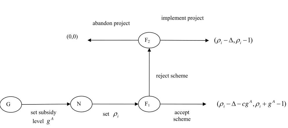
Figure 1a gives an extensive form representation of the automatic subsidy scheme. At G the government sets a fixed subsidy level per project, gA, where the A superscript indicates an automatic grant. At N a move by nature allocates the firm a project with productivity ρi. At F1 the firm can choose to accept or reject the subsidy. If the firm accepts, it must carry out the project with a pay-off to the government of (ρi-Δ-cgA) and to the firm of (ρi+gA-1).ix If the firm rejects the subsidy at F2 it can then either abandon the project, with pay-offs of (0,0), or implement it unaided where the pay-offs are (ρi-Δ,

ρi-1).

Using backward induction, at F1 with a positive subsidy offer, the firm will never reject the scheme and then implement the project. Therefore all projects where:

(5) A 1 0

i g

ρ + − ≥

accept the scheme, implement the project and receive the subsidy. Where the productivity

lies in the range 1 A,1

)

i g

ρ ∈ −⎡_⎣

With an automatic scheme, the government sets the fixed subsidy level to maximise expected welfare. The following general notation is introduced. The lowest productivity

level for which a firm will choose to enter the subsidy scheme is given as ρA_{, so that}

imposing expression (5) as an equality gives:

(6) A 1 A

g

ρ = −

(7)

1 _{(1 )(1 2 )}

1 (

( ) ( )

1 2(1 ) 2(1 )

i

i

A A A A

A

i i

g g

E NB d

r r ρ ρ ρ ρ ρ ρ ρ = =

− + − Δ _{− Δ −}

= − Δ = =

+

∫

2(1 ) )

r +

and the expected transaction cost as

(8)

1 _{(1 )}

1 (

( )

1 1

i

i

r A A _{A A}

A A

i

cg r _{cg r g}

E T cg d

r r ρ ρ ρ ρ ρ = + = + − ₊ = = = +

∫

Equations (7) and (8) express the expected net resource benefit and transaction cost as functions of the subsidy level. Reformulating equation (2) to reflect expected net resource benefit, it is straightforward to derive the optimal subsidy rate using the first and second order conditions. However, for pedagogic reasons, the marginal values of the expected net resource benefit and transaction cost of increasing the subsidy rate are determined separately. This procedure has two advantages: it allows a diagrammatic exposition and eases the welfare comparison of an automatic and discretionary subsidy.

Here, and at various other points in the paper, it is convenient to derive the expected outcomes not for an individual project but for projects submitted by a population of (1+r) firms, each with one project.x Adopting this procedure and partially differentiating equations (7) and (8) with respect to the subsidy rate gives the expected marginal net benefit and cost for changes in the level of the automatic subsidy. These will be subsequently referred to as the marginal benefit and marginal cost of the subsidy.

(9) ( ) ( ) 1

A

A A

A

E NB

ME NB g

g

∂

= = − Δ −

∂

(10) ( ) ( ) ( 2 )

A

A A

A

E T

ME T c r g

g

∂

= = +

∂

Setting marginal benefit and cost equal gives the optimal automatic subsidy, ,

as

*

A

g

xii_:

(11) * 1

1 2

A cr

g

c − Δ − =

+

The corresponding optimal change in welfare is shown as the area of the triangle between the marginal benefit and cost curves. It is calculated as:

(12)

* 2

* (1 ) (1 ) (1 2 )( )

( )

2 2(1 2 ) 2

A A

A cr g cr c g

E W

c

− Δ − − Δ − +

= = =

+

* 2

A number of basic points are clear from inspection of Figure 2. First, with no transaction cost, so that c is set to zero, the optimal automatic subsidy is 1 – Δ, reducing the subsidised financial cost of inputs to their shadow price. Second, with any increase in transaction cost, either through an increase in the cost of public funds, c, or the extent of non-additionality, r, the optimal subsidy and additional welfare falls, so that:

* * _{( )} * _{( )} *

, ,

A A A A

g g E W E W

c r c r

∂ ∂ ∂ ∂

0

<

∂ ∂ ∂ ∂

Third, if the fixed marginal transactional cost of subsidising the non-additional projects, cr, is greater than the marginal resource benefit from projects on the verge of profitability, 1-Δ, then the optimal strategy is to offer a zero subsidy.

4. A discretionary scheme with accurate appraisal

Consider next a discretionary scheme with no appraisal error. The game is set up as in Figure 1b. The government moves first, at G1, by announcing a subsidy schedule that sets the non-negative subsidy level for an individual project as a function of the productivity signal:

(13) ( )gi =g si

At N1 there is a move by nature that randomly allocates the firm a project with productivity level, ρi, which is private information to the firm. At F1 the firm then decides whether to accept or reject the scheme. If the firm rejects the scheme, at node F2 it chooses either to implement the project or not. The pay-offs at this point are in principle the same as the corresponding pay-offs under the automatic subsidy. However, for pedagogic purposes, the pay off to the firm if it implements the project unaided is taken to be ρi− +1 ε , where ε is vanishingly small.

xiv

Up to this stage in the game, there is no transaction cost. However, once the firm accepts the subsidy scheme, there is an appraisal procedure that costs the government k per project and requires the firm to make a resource commitment of β. If the project goes ahead, the total cost to the firm is still unity. However, if the project is not implemented then the firm looses the committed resources.

In order to compare more easily discretionary schemes with accurate appraisal and with appraisal error, the appraisal procedure is identified with a move by nature at N2. Here this produces a productivity signal, DA

i

s , where the DA superscript stands for a

discretionary subsidy with accurate appraisal. The definition of accurate appraisal is that the productivity signal equals the actual project productivity, so that:

(14) DA

i i

s =ρ

To find the optimal subsidy schedule - that is the optimal form of expression (13) - first consider the incentive compatibility constraint at F3 (Grossman and Hart, 1983). For the firm to accept the subsidy requires:

(15) 1ρ_i− +g_i ≥ −β

Next, using backward induction at F2, the firm’s participation constraint at F1 is that: (16) 1ρ_i− +g_i ≥Max(ρ_i− +1 ε,0)

The government’s initial step in deriving the optimal subsidy schedule is to satisfy the firm’s incentive compatibility and participation constraints at minimum cost.

Expression (16) suggests that a separation should be made in the analysis, depending on whether the inequality ρi – 1 ≥ 0 holds. Where this inequality does hold, the project would be implemented even if unassisted. The government therefore offers a subsidy of zero:g_i =0.

On the other hand, where ρi – 1 < 0 for the project to be implemented, a subsidy is required. In this case, the lowest cost subsidy consistent with the participation constraint is given as:

(17) 1gi = −ρi

This subsidy level is also consistent with the firm’s incentive compatibility constraint (equation (15)). Substituting equation (17) into equations (2), (3) and (4) gives the government’s “lowest cost” pay-off from subsidising a project whose productivity lies within this range as:

(18) (1W_i =ρ_i− Δ −c −ρ_i)−k(1+c)

Imposing the government’s participation constraint (Wi ≥ 0) in equation (18) generates the range of productivity values that optimally attract a subsidy as:

(19) 1

1 i

c k c

ρ Δ +

> ≥ +

+

offer a subsidy that fails to meet the firm’s participation constraint.xv Again a zero subsidy is convenient.

Following these arguments, the optimal form of expression (13) is therefore:

(20) , 1

0

DA DA

i i

i

,

i

If s s s g s

else g

> ≥ = − =

where

1

1

DA DA c

s and s k

c Δ +

= = +

+

This optimal subsidy scheme has characteristics that are reflected in the rules for RSA. In

particular, the UK government aims only to subsidise additional projects, so that DA

s = 1,

and the subsidy is the minimum required for the project to be profitable, . The

determination of

1 i

g = −s_i

DA

s is a more uncertain. RSA applications where the grant is greater

than £250,000 “ are required to satisfy an explicit test of economic efficiency to ensure that the project will confer some net benefit to the UK economy” (Scottish Executive, 2006, p. 4). Projects where the grant is likely to be greater than £2 million are put through an even more detailed efficiency test and, if necessary, a fuller cost benefit appraisal. However, there are also imposed aid ceilings for RSA, where the maximum level of aid varies across different sub-regions. In Development Areas in Scotland, the maximum grant level varies between 10% and 30% of project costs in.

From equations (14) and (17) it is clear that there is a very straightforward mapping between the project’s actual productivity, the productivity signal and the subsidy offer. In particular, corresponding to the range of productivity signals that will attract a subsidy, there is an identical range of project productivities within which the firm will enter the subsidy scheme. This range of productivities is again bounded by the minimum and

maximum values: ρDA,ρDA

)

⎡⎣ . Therefore in the accurate appraisal case:

(21)

1 DA DA c

s k

c

ρ = = Δ + +

+

(22) DA DA 1

s

with the corresponding optimal minimum and maximum values for the discretionary subsidy:

(23) * 1 _, * ₀

1

DA DA

g k g

c − Δ

= − =

+

The increase in expected welfare, E(W), from operating the subsidy scheme can be decomposed into the expected net resource benefit and transaction cost.

(24) 1 1 ( ) ( ) 1

(1 )(1 2 ) _{(2(1 ) )}

2(1 ) 2(1 )

i DA i

DA

i i

DA DA DA D

E NB d

r

g g

r r

ρ

ρ ρ ρ ρ

ρ ρ

= =

= − Δ

+

− + − Δ _{− Δ −}

= = + +

∫

( ) ( (1 ) (1 ))

1

(1 )

1 1

(1 )(1 ) (1 )

1 2 1 2

i DA i DA i i DA DA DA D

E T c k c d

r

c g c

k c k c g

r r ρ ρ ρ ρ ρ ρ ρ = = = − + + + A ⎡ _{⎡ ⎤} ⎤ ⎡ − ⎤ _{⎢ ⎣ ⎦ ⎥} = _⎢ + + − _⎥= + + ⎢ ⎥ + _{⎢⎣ ⎥⎦} + ⎣ ⎦

∫

Again, applying the policy to a population of 1+r projects, differentiating (24) and (25)

with respect to DA

g gives the marginal benefit and cost for changes in the maximum

subsidy for a discretionary scheme with perfect appraisal.

(26) ( ) ( ) 1

DA

DA D

DA

E NB A

ME NB g

g

∂

= = − Δ

∂ −

(27) ( ) ( ) (1 )

DA

DA D

DA

E T A

ME T k c cg

g

∂

= = + +

∂

To begin, note that interchanging gA with DA

g in equations (9) and (26) reveals that

element, k(1+c) is the resource and tax cost associated with the appraisal. The variable

element, DA

cg , is the cost of the tax to financial marginal projects.

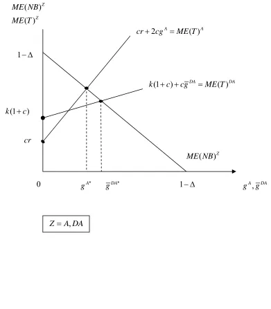
The relevant marginal benefit and cost curves for the discretionary subsidy with accurate appraisal are also shown on Figure 2. The optimal discretionary subsidy is found where they intersect. In general, the optimal levels for the maximum discretionary and automatic subsidies differ. Algebraically these expressions are given in equations (11) and (23). As with the automatic subsidy, that area of Figure 2 between the marginal benefit and cost curves represents the welfare gain. This has the value:

(28) * (1 (1 )) * (1 (1 ))2 (1 )( )

2 2(1 )

DA DA

DA k c g k c c g

W

c

− Δ − + − Δ − + +

= = =

+

* 2

2

It is clear by inspection that any increase in transaction cost, in this case the appraisal cost, k, and the cost of public finance, c, will again reduce the optimal maximum grant and the expected welfare change:

* * _{( )} * _{( )} *

, , ,

DA DA DA DA

g g E W E W

c k c k

∂ ∂ ∂ ∂

0

<

∂ ∂ ∂ ∂

Further, Figure 2 also indicates that there might be no possibility for a welfare increasing discretionary subsidy. This would be where the fixed marginal appraisal cost, k(1+c), is greater than the maximum possible marginal net resource gain, 1–Δ.

An examination of Figure 2 shows that there is no a priori reason for believing that

the discretionary subsidy with perfect appraisal produces higher welfare gains than an optimal automatic subsidy. From inspection, cr > k(1+c) is sufficient for the discretionary

subsidy to have a higher welfare gain, whilst A* D

g >g A*is sufficient for the automatic

subsidy to have the higher welfare. In general the relative welfare gain depends on the trade off between the greater revenue-raising costs associated with the automatic subsidy against the potentially greater appraisal costs of the discretionary subsidy.

The accurate appraisal scheme has the following important features. First, there is perfect separation: no “non-additional” projects apply for the subsidy. Second, all additional projects that generate a welfare benefit apply, whilst no additional project whose subsidisation would generate a welfare loss applies. Third, firms enjoy no information rent: all the benefit from the subsidy scheme goes to the government. Finally, all projects that apply are implemented. However, in general, none of the above characteristics apply once appraisal error is allowed.

Appraisal error is introduced in the following way. Where a project with productivity

ρi is being appraised, the productivity signal takes a symmetric, uniform distribution with maximum and minimum values of ρ α_i+ and ρ α_i − .xvi This distribution is common knowledge. The game represented in Figure 1b is adjusted accordingly. The move by

nature at N2 now generates the productivity signal, DE i

s , in the random manner as

described. The superscript DE indicates a discretionary scheme with appraisal error. All other elements of the game are as before.

For accountability, the subsidy schedule is given by equation (20). It is identical to that used in the accurate appraisal model. In effect, this procedure requires that the government treat its own appraisals as accurate. This implies that a project should be offered a positive subsidy only where the appraisal suggests that this is appropriate. Further, the project should be given the minimum subsidy required for project viability given the productivity signal. As argued in the introduction, this reflects existing UK practice on the administration of RSA (Scottish Executive, 2006).

than its actual level. Third, there might be additional welfare improving projects that no longer meet the participation constraint once errors are introduced into the appraisal procedure. Finally, because firms can accept those subsidy offers that produce excess profits but reject those that produce a loss, generally firms will make positive profits from entering the scheme. As will become apparent, expected profits also occur where a project’s productivity is close to the upper bound signal, DA

s : that is, close to unity. All

these changes that accompany appraisal error reduce the efficiency of the discretionary subsidy scheme.

The values of two key parameters, expressed relative to the appraisal error, α , determine the change in the efficiency of the discretionary scheme that accompanies

appraisal error. These parameters are the value of the maximum grant, DA

g , and the

firm’s committed cost, β. The nature of these effects can be investigated by first considering a situation where the maximum subsidy and the committed costs are large,

relative to the appraisal error, so that 2

DA

g

α ≥ and 1

β

α ≥ .

xvii

5.1 Relatively small appraisal error: 2, 1

DA

g β

α ≥ α ≥

Begin with a project whose possible productivity signals all lie within the aided range, so that:

(29) 1 DA D

i i i

s ρ α ρ ρ α s

= > + > > − ≥ A

i

At F3 in Figure 1b the firm accepts the subsidy offer only if the incentive compatibility constraint, inequality (15), holds, with the subsidy being determined by equation (20), but in this case the signal is equal to:

(30) s_i =ρ α_i+

Given that in the case under consideration the signal lies within the range DA, DA

)

s s

⎡⎣ ,

(31) β α≥ i

The most straightforward situation, and the one that will be the focus of the discussion in the text, is where the size of the maximum error is less that the committed costs. This is given as:

(32) β 1

α ≥

The alternative case, where inequality (32) fails to hold, is dealt with in Appendix 1. The assumption of relatively high committed costs makes the analysis more tractable. But more importantly, when the model is calibrated to stylised facts about the operation of UK regional subsidies, the observed outcomes are consistent with a high committed costs.

If inequality (32) holds, then for any project that receives a positive subsidy offer, the incentive compatibility constraint holds too. For projects that lie within the range given by expression (29), the expected profitability of entering the scheme is calculated, using equations (1) and (20), as:

(33) ( ) 1 ( ) 0

2

i i i i

s

i _s i i

E ρ α s

ρ α

π ρ

α

= +

= − dsi

=

_∫

In this case the expected value of the subsidy just equals the unassisted loss. In this range of productivities, the introduction of error into the appraisal process has no impact on the expected outcome. The incentive compatibility condition always holds at F3 and the participation constraint holds at F1 with expected profit at a minimum value.

However, for projects whose productivity is closer to the lower or upper bound

signal values, that is, where DA, DA

)

ρ ∈⎡_⎣ +α or ρi∈ −(1 α,1), the appraisal error does

Begin where the project productivity is ρi = −1 φ, where 0< <φ α. In this instance

the project productivity is close to the upper bound productivity signal, 1. The expected profitability is given by the expressionxviii:

(34)

2 1

1

1 (

( ) 1 (1 ) 0

2 4

i i

s

i i i i

s

E s ds

φ α

α φ

π ρ φ

α α

= = − −

+

= − +

∫

A project close to the upper bound signal will not get a subsidy offer where the appraisal wrongly identifies the project as being non-additional. However, it still receives subsidy offers above the minimum required level for viability when the productivity signal is below the actual productivity. But for the net impact of the subsidy scheme on the firm’s profitability to be zero, the firm would have to pay a penalty when the productivity signal is greater than one. Simply giving a project with a non-additional appraisal a zero subsidy means that the firm’s expected profitability becomes positive. This is welfare reducing in so far as the additional subsidy has to be funded and therefore the cost of raising tax revenue is increased.

On the other hand, where the project’s productivity is close to the lower bound

signal, so that DA i s

ρ = +ϕ, where ϕ α≤ , expected profitability is adversely affected and

is therefore always negative.xix The scheme now fails to satisfy the firm’s participation constraint at F1. The intuition here is straightforward. Where the lower bound signal, _sDA_, is within the project’s range of possible productivity signals, some of these potential high subsidy payments that such a project could attract are ruled out. Hence the participation constraint is not met. This implies that for the discretionary scheme with appraisal error

where β 1

α ≥ and 2 DA

g

α ≥ the lower bound productivity level where firms will enter the

scheme is given by:

(35) DE DA

s

ρ = +α

it will accept.xx This implies that the upper bound productivity level for entering the discretionary scheme with appraisal error is:

(36) ρDE = +1 α

For a non-additional project whose productivity level lies in the range

[

)

probability of receiving a subsidy is1 2

i

ρ α α

− +

and the expected value of that subsidy

would be:

2

(1 )

( )

4 i i

E π ρ α

α

− +

= .

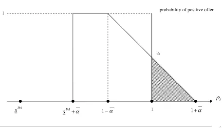
If 2

DA

g

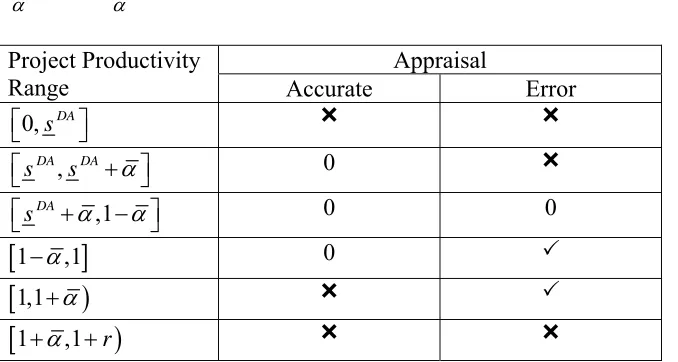
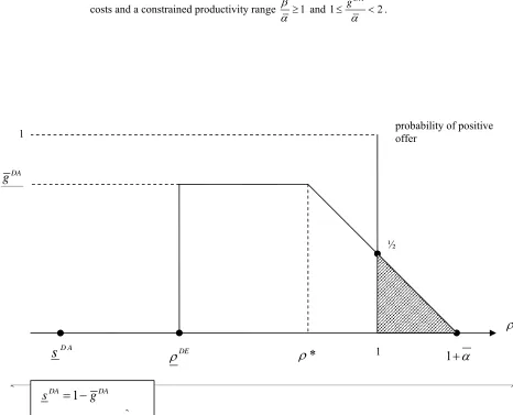
α ≥ , Figure 3 gives the probability that a project with productivity ρi would receive a positive subsidy. This is the product of the probability that a firm with such a project would apply and the probability that such a project would receive a positive offer, conditional on its applying. Table 1 summarises the results for the accurate appraisal and

appraisal error discretionary schemes constructed for the parameter values β 1

α ≥ and

2

DA

g

α ≥ . This table shows whether a project whose productivity lies within a particular

band will participate in each discretionary subsidy scheme. It also identifies those productivity ranges where the expected subsidy payment adds to the counterfactual level of profits. This occurs for additional projects where the expected profits are positive and for non-additional projects where the expected subsidy payment is positive.

It is apparent that in this case the introduction of appraisal error moves the range of

project productivities that meet the firm’s participation constraint, ρDE,ρDE

)

⎡⎣ , upwards by the value α. This indicates two important sources of inefficiency introduced with appraisal error. The first is the additional projects that are lost to the scheme where

)

DA DA i s s

ρ _{∈ ⎣}⎡ +α . The second is the additional administration and tax raising costs

where ρ_i∈

[

)

error is the tax funding of the positive profits made by projects where ρ_i∈ −(1 α,1).

5.2 Relatively low maximum subsidy: 2, 1

DA

g β

α < α ≥

A reduction in the relative size of the maximum grant, so that 2

DA

g

α < , slightly

complicates the analysis. One implication is that a project at the lower bound

productivity, ρDE_{, generates a range of productivity signals that includes both the upper}

and lower bound signal constraints. That is to say, a project with the lower bound productivity has a positive probability of receiving a zero subsidy offer both because its productivity signal might be too low and also because it might be too high. This is analysed in Appendix 2. The lower bound productivity level is now given as:

(37)

2

1 4

DA DE g

ρ

α

⎡ ⎤

⎣ ⎦

= −

The probability that a project entering the scheme will receive a positive subsidy is also more complex with this more limited range of acceptable subsidy signals. For the range of productivity values where the project does not encounter the lower bound signal

constraint, 1 1 DA i g

ρ α

> ≥ − + , the probability of getting a positive subsidy offer is

1 2

i

α ρ α

+ −

. For projects in the range 1 DA 1 i

g α ρ

− + > ≥ − DA

g , the probability of a

positive subsidy is 2

DA

g

α .

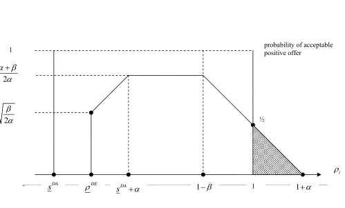
xxi _{The probability of receiving a positive subsidy where}

2

DA

g

α

> ≥1 is presented in Figure 4.xxii Again the inefficient loss of potential welfare

The importance in this model of the relative size of the maximum discretionary grant is consistent with empirical work on the impact of RSA by Criscuolo et al. (2007). Their

most favoured statistical model identifies no statistically significant effect of receipt of RSA on firm employment in those UK regions where the Net Grant Equivalent (NGE) - the maximum investment subsidy – is 10%. However, in assisted areas where the NGE is 20% and above, significant positive effects on employment are consistently found. The high proportionate non-additionality and the low values for the probability of receiving a positive subsidy offer for additional plants are likely to generate statistically insignificant effects.

6. Comparison of the discretionary subsidy with and without appraisal errors.

It is clear from Figures 3 and 4 that introducing appraisal error reduces the efficiency of the discretionary subsidy scheme and that the greater the error, the lower the expected welfare gain. These welfare losses are calibrated using stylised facts concerning the operation of discretionary subsidies. However, it must be emphasised that the results should be regarded as indicative orders of magnitude only.

A number of ex post evaluation studies using industrial survey data have attempted to

determine the degree of non-additionality in discretionary schemes. These studies generally produce a value of around 50% (HM Treasury, 1995).xxiii _{This means that} amongst projects receiving a positive subsidy, the number of additional projects should broadly equal the number of non-additional projects.xxiv The extent of non-additionality can be used to fix the relationship between the degree of error, α , the lower bound

productivity signal, DA

s , the lower and upper bound productivity level that meets the

firm’s participation constraint, _ρDEand _ρDA, and the expected welfare gain that would

The number of non-additional aided schemes, DE NA

N , can be expressed as a function of

α : (38) 1 1 1 (1 ) 2 4 i i DE

NA i i

N d

ρ α

ρ

α ρ α ρ α

= +

=

=

_∫

The very low number of non-additional projects relative to the value of α indicates that if the additional aided projects are to be of an equal number, the range for acceptable productivity signals must be less than 2α. Using the arguments following equation (37),

the number of additional aided schemes, DE A

N , is given by:

(39)

2 _{1 ( 1)( 1)}

1

4 2 2 2

DE A

m m m m

N =α⎡⎢_⎢⎡ − +m ⎤_⎥ + _⎢⎡ + − ⎤_⎥⎥⎤

⎣ ⎦

⎣ ⎦

⎣ ⎦

where:

(40) m gDA

α =

so that in the case under consideration, Setting equation (38) equal to equation (39) and solving numerically gives a value of m equal to 1.3. From equations (36), (37)

and (40), the values for

2> ≥m 1

, ,

DE DE D

s

ρ ρ A _and DA

g are 1 0.42 ,1− α +α,1 1.30− α and 1.30α

respectively.

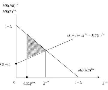
These results are sufficient to calculate the standard deadweight loss due the reduced range of subsidised additional projects, DE

DW

R .xxv Figure 2 shows the welfare benefit of the

discretionary subsidy scheme with accurate appraisal as the area between the marginal benefit and cost curves. With appraisal error, the number of projects that apply is reduced

by the ratio 1 0.42 0 1.30

− = .68 . This generates a deadweight loss, relative to the scheme with

accurate appraisal, equal to the welfare triangle indicated in Figure 5. The proportionate reduction is 0.682 = 0.46, so that:

(41) DE _0.46 D *

DW

R = W A

Given the value of DA

g , equation (28) can be employed to derive the welfare that

would be generated by a discretionary subsidy with accurate appraisal, DA*

W . Using an

estimate for the administration and distortionary costs of raising taxation, c, of 0.5 (Wren,

2007a), DA*

W . is given as:

(42)

[

] [

]

2

* 1.30 1 _1.27 2

2

DA c

W = α + = α .

Using the information on the upper bound productivity value with appraisal error, the second potential source of welfare loss relates to the additional tax-raising costs associated with financing the non-additional grantsxxvi.

(43)

1 ₂

2 *

1

(1 ) 0.03

4 24

i

i

DE D

NAT i i

c

R d

ρ α

ρ

α

ρ α ρ

α

= +

=

=

_∫

W

Official evaluations emphasise identifying the expenditures made for non-additional projects, with the aim of attempting to reduce the non-additional expenditure. However, equation (43) suggests that, in this model at least, the welfare loss on this score is relatively low.

The third source of inefficiency is the cost of financing the profits on the additional projects. The details of this calculation are also shown in Appendix 3. Its value is given as:

(44) DE _0.031 2 _0.02 D *

APT

R = α = W A

Again these additional tax-raising costs are low, relative to the additional welfare that would be generated by a discretionary subsidy with accurate appraisal.

The final step is to take into account the additional administration costs generated through the need to appraise the non-additional projects. Once more the details of this calculation are given in Appendix 3. The loss of welfare as a result of the costs of appraising non-additional projects once appraisal error is introduced is given by

(1 )

k c

(45) DE _0.08 D *

NAA

R = W E

Summing these costs indicates that the appraisal errors generate a decline of almost 60% in the welfare derived from the discretionary subsidy. The fall mainly comes from the reduction in the number of projects that apply.

6.Conclusions

This paper uses a stylised model to compare the efficiency of automatic and discretionary government grant schemes. Though abstract, the research is motivated by the practical issues that have emerged in the operation of UK regional policy. The effectiveness of the schemes has been measured primarily from a welfare (or cost benefit) perspective. The key findings are these.

For automatic subsidies and discretionary subsidies with no appraisal error, the relative welfare impact depends on a trade-off between the higher administration cost per project for discretionary subsidies as against the higher tax raising costs of financing grants to non-additional projects with automatic subsidies.

The introduction of appraisal error reduces the effectiveness of the discretionary subsidies: calibrating the present model to stylised facts taken from UK ex post industrial

survey evaluations, the welfare gain from the discretionary scheme is more than halved. The main cause for concern over appraisal error is usually the extent of non-additionality. However, with the parameter values used here, the additional administrative and tax raising welfare costs associated with non-additionality are relatively small. Rather, in this model the main welfare loss stems from the restricted number of projects entering the scheme because the scheme no longer meets the firm’s participation constraint for lower productivity projects. In the model this is linked to the need for accountability in the administration of discretionary aid. This source of welfare loss is particularly difficult to identify in empirical studies.

However, the analysis raises a number of unanswered questions. The first relates to the high level of non-additionality identified in empirical, typically industrial survey, evaluations. This suggests that the error in the appraisal procedure is high relative to the optimal maximum grant. This result has the implication that the number of rejected projects (projects that receive a zero subsidy offer) should be very large – greater than the number of projects that receive positive grant offers.xxvii There is no evidence that such a large proportion of applicants fail to receive positive assistance. However, the procedure for applying for RSA is rather more protracted than implied here and firms are recommended to make informal approaches initially to the relevant government department. This may be where many projects are turned away.

The second problem is that the implicit high relative appraisal error, and the corresponding small range of project productivities over which the firm will enter a discretionary scheme, leads to a situation where all firms that apply implement the project whether they receive a positive grant offer or not. This contradicts previous evidence on the operation of RSA that suggests that some projects that are given a zero grant offer do not subsequently implement the project (Allen et al, 1986).

A third issue concerns the potential conflict between economic efficiency and accountability that is embedded in the analysis in this paper. These, albeit indicative, results suggest that with appraisal error, the range of additional productivity signals that the government is prepared to subsidise should be increased above that which would be optimal with accurate appraisal. If this is a major source of inefficiency associated with inaccurate appraisal, can this be solved through more sophisticated government practice?

Fourth, if appraisal error is negatively related to the appraisal costs, an optimising subsidy scheme would also incorporate the optimal level of appraisal activity (Wren, 2007a). This is an issue not tackled in this paper

APPENDIX 1: The analysis with relatively low committed costs: β α<

This appendix outlines the operation of a discretionary subsidy with appraisal error

where β 1

α < and 2 DA

g

α ≥ . Initially consider a project whose productivity, ρi, is such that all possible productivity signals lie within the aided range, so that expression (29) of the text holds. In this case, for values of αi greater than β, at F3 the firm’s incentive compatibility constraint is not met: the subsidy offer is inadequate and the firm will reject. In this range, the proportion of projects made an offer that they reject is given as λ, where:

(A1.1)

2

α β λ

α

− =

Consider next the firm’s participation constraint at F1. The expected profitability E(πi) is:

(A1.2)

2

1 (

( ) ( ) 0

2 4

i i i i

s

i _s i i i

E ρ β s ds

ρ α

α β

π ρ β

α α

= + = −

+

=

∫

which is always positive. This reflects the fact that the firm does not now accept subsidy offers below a certain level and therefore extracts an information rent.

Equations (A1.1) and (A1.2) characterise projects whose productivity lies within the range given by expression (29). However, because the firm will reject offers where the productivity signal is greater than ρi + β, then equations (A1.1) and (A1.2) actually apply to a wider range of project productivities, that is where:

(A1.3) DA 1 D

i i i

s = ≥ρ β ρ+ > >ρ α− ≥ s A

Projects whose productivity levels satisfy expression (A1.3) are not affected by the discontinuities introduced by the government’s restricted productivity signal range

)

s s

⎡⎣ , imposed for accountability considerations. In productivity ranges closer to these upper and lower subsidy bounds, the outcomes generated by the subsidy regime differ. This is represented in Figure A1. This figure gives the range of productivities for

which a firm will apply for the discretionary subsidy with appraisal errors ρDE,ρDE

)

also shows for each productivity level within this range the probability that the project will be offered a positive subsidy that will meet the firm’s incentive compatibility constraint i.e. that the firm will accept. For productivity values outwith the range

)

s s

⎡⎣ the analysis is exactly the same as in the main text.

To determine the lower bound productivity level that just meets the participation

constraint, ρDE_{, consider the probability that the project will be offered a subsidy that}

satisfies the incentive compatibility constraint at F3 and the expected value of that offer,

given the value of DA

s . Define ρDE as sDA+γ . The value of γ is then determined by

imposing the participation constraint as an equality:

(A1.4)

2

1 (

( ) ( ) 0

2 4

i i i i

s

i _s i i i

E ρ β s ds

ρ γ

γ β

π ρ β

α α

= + = −

+

=

∫

which implies that:

(A1.5) γ =2 αβ β−

so that:

(A1.6) DE DA 2

s

ρ = + αβ β−

For the range of productivity values DA 2 , DA

)

s αβ β s α

⎡ _{+ − +}

⎣ entry into the scheme

meets the firm’s participation constraint, but the range of productivity signals is restricted

from below by the minimum signal, DA

s . The probability that the firm will receive an

offer that meets the incentive compatibility constraint where the productivity level lies

within this range is 2 DA i s ρ β α − +

which has minimum and maximum values of

, 2

β α β

α α

⎡ + ⎞

⎟

⎢ _⎟

⎣ ⎠. For projects within this range there are three potential sources of

expected profits for the firm from the subsidy scheme are positive, so that the average cost per project of government finance is increased.

In the range of productivities DA ,1

)

s α β

⎡ + −

⎣ expression (A1.4) holds and the

probability of receiving an acceptable positive offer is 2

α β α

−

. The sources of welfare

loss are again the lower implementation level of welfare-improving projects, the resources committed to the appraisal procedure by both firms and government for the projects that fail to meet the incentive compatibility constraint, and the funding of the higher expected profits.

Finally projects whose productivities lie in range

[

)

match the high committed cost case analysed in the text. Projects with productivities in this range will always satisfy the incentive compatibility constraint at F3. Even if the project is given a zero subsidy, the loss from implementing the project is less than the loss from abandoning it, given that a proportion of the costs, β, are already committed. The key issue is therefore whether the project passes the participation constraint at F1. Given that all projects in this range will be implemented, the expected profitability is:

(A1.7)

2

1 ( 1 )

1

( ) 1 (1 ) 1 0

2 4

i i i

s

i

i i _s i i i

E s ds

ρ α

α ρ

π ρ ρ

α α

= = −

+ −

= − +

_∫

where 2 2 ( ) ( ) , 0 i i i i

E π E π

ρ ρ

∂ ∂ _>

∂ ∂

This means that all projects in this range will apply for the subsidy scheme and all will be implemented. The only source of inefficiency for these projects, as compared to the accurate appraisal scheme, is the tax raising cost required to finance the additional profits. Although the expected profitability of projects increases as the productivity approaches unity, the probability of getting a positive subsidy offer falls. This is the probability that

APPENDIX 2: The lower bound productivity where 2

DA

g

α <

Express this productivity in terms of two parameters γ γ₁, ₂, where:

(A2.1) DE DA ₁ 1 ₂

s

ρ = + = −γ γ

with α γ γ≥ ₁, ₂ ≥0. At ρDE_{, the firm’s expected profitability from entering the scheme}

equals zero. At F3 the incentive compatibility constraint is always met. This means that the expected grant value just equals the unsubsidised loss, so that:

(A2.2) 2

(

)

1

2

1 2

2 2

1

( ) (1 ) 0

2 4

i i i i

s

i _s i i

E ρ γ s ds

ρ γ γ γ π γ α α = + = − +

=

_∫

Rearranging equation (A2.2) produces:

(A2.3) γ γ₁+ ₂ =2 αγ₂

If :

(A2.4) ₂ DA

ng

γ =

and given that from (A2.1):

(A2.5) _{1 2} DA

g

γ γ+ =

then equation (A2.3) produces:

(A2.6) 4 DA g n α =

Substituting expression (A2.6) into (A2.4) and then into equation (A2.1) gives the value for the lower bound productivity:

(A2.7) 2 1 4 DA DE g ρ α ⎡ ⎤ ⎣ ⎦ = −

which is equation (37) in the text.

APPENDIX 3: Calculating the welfare loss from appraisal error

A3.1 Determining N_ADE

Using the arguments following equation (37), the value of additional aided schemes,

DE A

N , is given by:

(A3.1)

2

1 1 (

1 ( 1)

1 4 1 (1 ) 2 2 i i i i m DE

A i i

m m

m

N d

ρ ρ α

ρ α _ρ α

1)

i

d

ρ α ρ ρ

α = = − = − − = − ⎡ ⎤ ⎢ ⎥ = _⎢ − + + _⎥ ⎢ ⎥ ⎣ ⎦

∫

∫

which gives equation (39) in the text.

A3.2 Determining DE

APT

R

The cost of financing the profits on the additional projects is calculated as:

(A3.2)

2 2

1 ₂ 1 ( 1) 1

2 1 ( 1)

1 1

4 4

1

(1 ) (1 )

4 4

i i i

i

i i

m DE

APT i i i i i

m m m

m

R c d d d

ρ ρ α ρ

ρ α _ρ α _ρ α

α

ρ α ρ ρ ρ ρ

α = = − − = = − − _{= − = −} ⎡ ⎤ ⎢ ⎥ = _⎢ − + + − − _⎥ ⎢ ⎥ ⎣ ⎦

∫

∫

∫

generating the expression:

(A3.3)

[ ]

2

1 1

3 2 2

1 ( 1) 1

1 ( 1) 4 1

4

(1 ) (1 )

12 4 2

i i

i i

i i

m

DE i i

APT i m

m m m R c ρ ρ ρ α α ρ α

ρ α ρ

ρ α _{α ρ} ρ

α = = = − − = − = − − = − ⎡ _{⎡ − + ⎤ ⎡ − ⎤} ⎤ ⎢ ⎥ = −_{⎢ ⎥} + − −_{⎢ ⎥} ⎢ _{⎣ ⎦ ⎣ ⎦} ⎥ ⎣ ⎦

which gives the result that:

(A3.4)

2

3 2 2 2

2 1 ₁ 1

12 4 4 2 4

DE APT

m m m m

R cα m

⎡ _{− ⎡ ⎤ ⎡ ⎤} ⎤

= ⎢ + _⎢ − + _⎥− _{⎢ ⎥} ⎥

⎢ ⎣ ⎦ ⎣ ⎦ ⎥

⎣ ⎦

Given the values c = 0.5 and m = 1.3:

(A3.5) DE _0.031 2 _0.02 D*

APT

This result is given as equation (44) in the text.

A3.3 Determining R_NAADE

The loss of welfare as a result of the costs of appraising non-additional projects once appraisal error is introduced equals αk(1+c). From equation (42) the proportionate

reduction in welfare, DE NAA

R , is given as:

(A3.6) 2(1 ) 3

(1 (1 ) )1.3 1.3( 1.5) DE

NAA

c k R

c k q

α α

+

= =

− Δ − + −

where q is the ratio of the maximum resource gain per project to the appraisal cost, so that:

(A3.7) q 1

k − Δ

=

It is not straightforward to fix a value for q. Again stylised facts are used, but to restate the earlier warning: the results should be treated as indicative, rather than definitive. For the UK, the maximum subsidy under the RSA scheme equals 30% of the capital costs (Scottish Executive, 2006). Given that capital costs typically are around 30% of value added this represents a grant of around 10% of the value of the project. This

would imply that the value of DA 0.1

g = . Substituting in this value to equation (23),

which determines the value of DA

g from the underlying parameters, and rearranging

gives:

(A3.8) q 0.15 1.5

k

= +

Table 1: Participation in a discretionary subsidy scheme and the expected profitability of the subsidy payment under accurate appraisal and appraisal error for the parameter values

1

β

α ≥ and 2

DA

g

α ≥ .

Appraisal Project Productivity

Range Accurate Error

0, DA

s

⎡ ⎤

⎣ ⎦ ³ ³

, DA DA

s s α

⎡ + ⎤

⎣ ⎦ 0 ³

,1 DA

s α α

⎡ + − ⎤

⎣ ⎦ 0 0

[

]

[

)

[

)

Figure 1a: An automatic subsidy scheme

implement project

set subsidy level A

g

set ρ_i

reject scheme abandon project

(0,0)

(ρi− Δ,ρi−1)

F2

( A, A 1)

i cg i g

ρ − Δ − ρ + −

N F1

G

Figure 1b: A discretionary subsidy scheme with accurate appraisal and appraisal error. abandon project implement project

(0,0) _{( , 1 )}

i i

ρ −Δ ρ − +ε

F2

announce scheme

g_i =g( )s_i

set ρ_i

reject scheme

accept

scheme set ( )

DE

i i

s =s ρ set g_i accept

offer

( (1− +c k) − −β β, )

reject offer

( (1 ) ,

1)

i i

i i

cg c k

g

ρ ρ

− Δ − − +

+ −

F1 N2

N1

G1 G2 F3

accurate appraisal set DA

i i

s =ρ

Figure 2: Marginal Net Resource Benefits and Transactions Costs to Automatic and Discretionary Subsidies

( )

( )

Z

Z

ME NB

ME T

1− Δ

(1 )

k +c

cr

2 A ( )A

cr+ cg =ME T

( )Z

ME NB

, A DA

g g

1− Δ *

DA

g *

A

g

0

,

Z = A DA

(1 ) DA ( )D

Figure 3: Probability of a positive offer for a discretionary subsidy with appraisal error with relatively high committed costs and an unconstrained productivity range,

1

β

α ≥ and 2

DA

g

α ≥ .

probability of positive offer 1

½

1+α

1

i

ρ

DA

s +α 1−α

DA

Figure 4: Probability of a positive offer for a discretionary subsidy with relatively high committed

costs and a constrained productivity range β 1

α ≥ and 1 2

DA

g

α ≤ < .

probability of positive offer

1

DA

g

½

DE

ρ

i

ρ

s

2

1 DA DA

Figure 5: Deadweight Loss from Appraisal Error

( )

( )

DA

DA

ME NB

ME T

1− Δ

(1 )

k +c

( )DA

ME NB

DA

g

1− Δ *

DA

g

0

(1 ) DA ( )DA

k + +c cg =ME T

0.32 DA

Figure A1: Probability of a positive acceptable offer for a discretionary subsidy

with relatively low committed costs and an unconstrained productivity range β 1

α < and

2

DA

g

α ≥ .

probability of acceptable positive offer

1

2

α β α

+

2

β

α ½

i

ρ

DA

s +α 1−β 1 1+α

DA DE

s ρ

2 DE DA

s βα β

= + −

References

Arup Economics and Planning (2000), Evaluation of Regional Selective Assistance, Arup

Economics and Planning, London.

Allen, K., Begg, H., McDowell, S. and Walker, G. (1986), Regional Incentives and the

Investment Decision of the Firm, HMSO, London.

Armstrong, H. and Taylor, J. (2000), Regional Economics and Policy, Blackwell

Publishing, Oxford.

Criscuolo, C., Martin, R., Overman, H. and Van Reenen, J. (2007), “The Effects of Industrial Policy on Corporate Performance: Evidence from Panel Data”, mimeo, Centre

for Economic Performance, London School of Economics.

Drazen, A. (2000), Political Economy in Macroeconomics, Princeton University Press,

Princeton, New Jersey.

Evans, D., Kula, E. and Sazer, H. (2005), “Regional Welfare Weights for the UK, England, Scotland, Wales and Northern Ireland”, Regional Studies, vol. 39, pp. 923-937.

Gillespie, G., McGregor, P.G., Swales, J.K. and Yin, Y.P. (2001), “The Displacement and Multiplier Effects of Regional Selective Assistance: A Computable General Equilibrium Analysis, Regional Studies, vol. 35, pp. 125-139.

Grossman S. and Hart. O. (1983), “An Analysis of the Principal Agent Problem”,

Econometrica, vol. 51, pp. 7-45.

HM Treasury (2003), The Green Book: Appraisal and Evaluation in Central

Government: Treasury Guidance, The Stationery Office, London.

Hart, M., Driffield, N., Roper, S and Mole, K. (2008), “Evaluation of Regional Selective Assistance (RSA) and its Successor, Selective Financ for Investment in England (SFIE)”, BERR Occasional Paper No. 2, Department for Business Enterprise and Regulatory Reform, London.

Holden D. and Swales, J.K. (1995), “The Additionality, Displacement and Substitution Effects of Factor Subsidies”, Scottish Journal of Political Economy, vol. 42, pp. 113 –

126.

King, J. (1990), Regional Selective Assistance 1980-1984, London HMSO

Layard, R. and Glaister, S. (1994), “Introduction” in R. Layard and S. Glaister eds., Cost

Benefit Analysis, 2nd edition, Cambridge, Cambridge University Press.

McVittie, E.P. and Swales, J.K.(2007), “”Constrained Discretion” in UK Monetary and Regional Policy”, Regional Studies, vol. 41, pp. 267-280.

PA Cambridge Economic Consultants (1993), Regional Selective Assistance 1985-1988,

London, HMSO.

Rose-Ackermann, S. (1999), Corruption and Government: Causes, Consequences and

Reform, Cambridge University Press, Cambridge.

Swales, J.K. (1995), “The Efficiency of Automatic and Discretionary Subsides”, paper presented to the Scottish Economic Society Conference, University of Aberdeen, April, 1995.

Swales, J.K. (1997), “A Cost-Benefit Approach to the Evaluation of Regional Selective Assistance, Fiscal Studies, vol. 18, pp. 73-84.

Viner, J. (1932), “Cost Curves and Supply Curves”, Journal of Economics, vol. 3, pp.

23-46.

Wren, C. (2007a), “Discretion in Industrial Assistance Schemes”, mimeo, Department of

Economics, University of Newcastle upon Tyne.

Footnotes

i _{In general UK regional policy has moved towards a more disaggregated and} decentralised system, shifting away from automatic subsidies to discretionary support. See, for example, the adoption by the post-1997 Labour Government of the Regional Development Agencies as central institutions in regional policy delivery (McVittie and Swales, 2007). At the time of writing, Regional Selective Assistance still applies in Scotland. The comparable scheme in England has been renamed Selective Finance for Industry in England (SFIE).

ii _{Essentially firms are assumed to be in atomistic competition (Viner, 1932) and it is} convenient to consider these domestic firms as operating in a large, perfectly competitive international market. For an alternative approach, see Holden and Swales (1995). For pedagogic reasons, issues such as displacement and multiplier effects (Gillespie, et al,

2001; HM Treasury, 2003, Wren, 2007b) are not considered here, but these could be incorporated in a straightforward manner.

iii _{Fraudulent behaviour, where the firm receives a grant for a project that is never} implemented, is ruled out.

iv _{The implication is that in making an application for a discretionary subsidy the firm has} to gather information that would be required anyway if the project goes ahead but has no value if it does not.

v _{An identical analysis applies if the market failure is in the product market. An example} would be where each project jointly produces a private and public good (Wren, 2007a).

Moreover, with the assumptions made in this paper, assigning zero cost to public funds would mean that the automatic subsidy would always out-perform the discretionary subsidy using the welfare criterion.

vii _{Again this assumption is made for ease of analysis. Differential income weights might} be one of the key reasons for regional subsidies (Evans et al, 2005; HM Treasury, 2003,

Annex 5). Also distributional issues will be relevant for income transfers to non-nationals, such as the shareholders of foreign owned companies.

viii _{The discretionary and automatic schemes broadly correspond to Regional Selective} Assistance and Regional Development Grants that have operated as elements of UK regional policy (Armstrong and Taylor, 2000). Wren (2007a) also considers a hybrid case “Proof of Need” scheme where the government adopts a relatively costly monitoring process but then offers a subsidy either of zero or of a fixed level.

ix _{The standard convention is adopted of listing the pay off to the first player (here the} government) first.

x _{There is not a problem in moving between considering the game as a single encounter} between a firm and the government, or as a repeated game where the government plays sequentially against a population of firms. In fact, credibility problems are likely to be reduced in the repeated game setting.

xi_{Excess expenditure is known as deadweight in the evaluation literature (HM Treasury,}

2003). However, this should not be confused with the conventional welfare economics notion of deadweight loss (Layard and Glaister, 1994).

xii _{Given that} 2

2 0

( )

A

A

NB g

∂ _<

∂ and

2

2 0

( )

A

A

T g

∂ _>