To appear inEngineering Optimization
Vol. 00, No. 00, Month 20XX, 1–22
Offshore Wind Farm Electrical Cable Layout Optimization
1
A.C. Pillaiab∗, J. Chicka, L. Johanningc, M. Khorasanchid, and V. de Laleub 2
aSchool of Engineering, The University of Edinburgh, Edinburgh, UK; 3
bEDF Energy R&D UK Centre, London, UK 4
cCollege of Engineering, Mathematics, and Physical Sciences, University of Exeter, Penryn, UK 5
dFaculty of Engineering, The University of Strathclyde, Glasgow, UK 6
(v6.0-R1 draft October 2014) 7
This article explores an automated approach for the efficient placement of substations and
8
the design of an inter-array electrical collection network for an offshore wind farm through
9
the minimization of the cost. To accomplish this, the problem is represented as a number
10
of sub-problems that are solved in series using a combination of heuristic algorithms. The
11
overall problem is first solved by clustering the turbines to generate valid substation positions.
12
From this, a navigational mesh pathifinding algorithm based on Delaunay triangulation is
13
applied to identify valid cable paths, which are then used in a mixed-inter linear programming
14
problem to solve for a constrained capacitated minimum spanning tree considering all realistic
15
constraints. The final tree that is produced represents the solution to the inter-array cable
16
results. This method is applied to a planned wind farm to illustrate the suitability of the
17
approach and the resulting layout that is generated.
18
Keywords:Offshore wind farm layout optimization; inter-array cabling; clustering;
19
pathfinding; capacitated minimum spanning tree
20
1. Introduction 21
Over the last decade the renewable energy sector has grown substantially and European 22
governments are now targeting high levels of renewable energy penetration in the forth-23
coming decade. In order to achieve these ambitious targets, many utilities are looking to 24
large offshore wind farms as part of the solution. Optimization of these large wind farms 25
has therefore arisen as a growing field of research for both developers and academics. 26
The layout optimization problem arises primarily due to the variation of wind speed 27
and therefore wind energy throughout a wind farm site. The variation is further intensi-28
fied as all wind turbines operating in the wind produce a wake, a region of air directly 29
behind the turbine where the wind speed is reduced and the turbulence intensity is in-30
creased. The effect of an upwind turbine’s wake decreases the further downwind that 31
a subsequent turbine is placed, however, the effect is still observed up to 20 rotor di-32
ameters downwind (Chamorro and Port´e-Agel 2010). Further complicating matters, the 33
cables that are needed to export the energy from each turbine have energy losses and 34
costs which are associated with the length of cable and the cross-section of the cable. 35
Also to be taken into consideration are the environmental and social constraints such 36
as the seabed geology, local marine species, visual impact, shipping routes, and fishing 37
areas to name a few. The layout optimization problem therefore becomes a problem of 38
balancing the energy extraction from the wind; the system losses; the project costs; and 39
the environmental and social constraints. 40
Many of the planned offshore wind farms in the UK, the Crown Estate Round 3 41
Projects, exceed 1 GW in installed capacity and are expected to consist of several hun-42
dred individual wind turbines. In existing offshore wind farms, the turbines tend to be 43
connected in strings of 5-10 turbines to a central collection point known as an offshore 44
high voltage substation (OHVS). These substations are in turn connected to grid connec-45
tion points onshore. As offshore sites offer little in regards to complex-terrain (i.e. hills, 46
valleys, etc.) the turbines have until now generally been placed in straight lines along 47
a regular grid. This, however, has not been optimized and early studies have indicated 48
that optimization of the turbine positions can lead to more efficient use of the wind farm 49
area (Fagerfj¨all 2010; Elkinton 2007). Existing tools have approached the optimization of 50
offshore wind farm layouts as a maximization of the energy yield and the minimization of 51
wake losses, however, it can more accurately be characterized from a utility perspective 52
as an optimization of the profitability of the generation asset or a minimization of the 53
levelized cost of energy (LCOE). With regards to this, it therefore becomes important 54
to consider all layout dependant aspects that either affect the energy yield of the wind 55
farm or the lifetime costs. 56
The electrical infrastructure impacts both the energy yield and the costs and therefore 57
has an important role to play in the optimization of offshore wind farms. The length of 58
cable and therefore the capital costs of the project are directly a function of the positions 59
of the turbines and the length of the cables also affects the energy losses that occur when 60
transmitting through the cables. Similarly these lengths of cable depend on where the 61
substations are placed relative to both the onshore connection point and the turbines. 62
The optimization of the collection network, the cables, and substations, therefore forms 63
an important component of the overall global optimization of an offshore wind farm 64
layout. 65
In the development of a tool to be used to optimize the layouts of offshore wind farms, 66
the problem of optimizing the electrical collection network for an offshore wind farm 67
has been examined. Considering the future UK Round 3 projects as a point of context, 68
the problem has been approached including as many realistic constraints as possible 69
and formulated using a combination of heuristics and mixed-integer linear programming 70
(MILP). As heuristics are used, this method may not reach proven optimality, but rather 71
reaches a good feasible solution in an acceptable run time. 72
This optimization problem includes the determination of the substation positions given 73
the realistic constraints faced by a developer, and the determination of the cable layout 74
given this substation position. The export cable, a component of the transmission net-75
work, is not considered as part of this optimization problem. 76
Previous work in this field has tended to look at small wind farms, or has omitted some 77
of the necessary constraints needed for the optimization of a real wind farm. Most have 78
elected to work only on a single construction phase of a wind farm with a single OHVS, 79
as subsequent phases and additional OHVS would follow the same procedure. 80
Fagerfj¨all (2010) implemented an MILP based approach for the electrical cable layout, 81
assuming that all the turbines were connected to a single substation. This approach 82
used a variation on the minimum spanning tree problem, a minimum Steiner tree, in 83
order to solve for the electrical cabling. A minimum Steiner tree is similar to a minimum 84
spanning tree, however, the arcs may branch anywhere along an arc and not only at 85
nodes. By approximating the problem to that of the minimum Steiner tree, the cable 86
length is therefore further minimized. Similar work has also been undertaken by Svendsen 87
(2013) and Lindahl et al. (2013) using a MILP implementation to solve for a capacitated 88
minimum spanning tree. Both of these studies, however, correctly identified that the 89
fact, the capacitated minimum spanning tree (CMST) problem is NP-hard and therefore 91
an optimal solution is not found in polynomial time, but rather exponential. The problem 92
therefore becomes exponentially complex as more turbines are added and more possible 93
cable arcs must be considered. 94
Due to the complexity, a number of studies have opted to use heuristic algorithms 95
such as genetic algorithms in order to optimize the electrical cable layout (Dutta and 96
Overbye 2011; Gonz´alez-Longatt and Wall 2012; Cerveira and Pires 2014; Li, He, and Fu 97
2008; Zhao, Chen, and Blaabjerg 2008, 2009; Lumbreras and Ramos 2013). These studies 98
have therefore sacrificed finding the proven optimal solution in favour of a good feasible 99
solution in acceptable time-scales. Bauer and Lysgaard (2013) simplified the problem to 100
only allowing strings of turbines without any branching, allowing a variation on a vehicle 101
routing problem algorithm to be applied. This too finds solutions in reasonable time-102
scales, however, by not allowing branching reduces the problem complexity significantly, 103
and eliminates many feasible solutions unnecessarily including potentially the optimal 104
solution. 105
Studies carried out by Dutta and Overbye (2011, 2012, 2013) have looked at using a 106
minimum spanning tree (MST) and applying the capacity constraints by running the 107
MST on clustered turbines representing the capacity constraints of the largest cross-108
section of cable. This work has also modified the MST to represent a minimum Steiner 109
tree. Dutta and Overbye (2013) also include an algorithm to account for exclusion areas 110
where cables may not be placed, by constructing convex hulls from the obstacle and 111
turbine positions to derive a shortest path. 112
Given the desire to apply the methodology to real sites, the electrical inter-array cable 113
optimization problem has been approached pragmatically, dividing the overall problem 114
into two sub-problems: the placement of the substations and then the determination of 115
the cable layout. The study at hand intentionally opted to continue on from the work of 116
Fagerfj¨all (2010); Svendsen (2013); Lindahl et al. (2013) using a MILP formulation for 117
the electrical cable layout problem and introduce additional constraints to represent the 118
realistic case of UK Round 3 sites. The new constraints introduced in this work take into 119
account complex geographical information systems (GIS) shapes as constraints and the 120
fact that cables may not cross in the offshore environment. Additional constraints have 121
also been explored to aid in reducing the computational time. 122
2. Process Overview 123
The design of offshore wind farms and the decision regarding the number of substations 124
to build is largely driven by the capital expenditure (CAPEX) associated with build-125
ing a substation along with the necessary foundation works. Projects tend therefore to 126
minimize the number of substations such that substations are efficiently designed with a 127
minimum surplus capacity. The total number of substations is therefore often predeter-128
mined based on the number of construction phases or the total wind farm capacity. 129
As a result of this, the decision of where to place the substations is effectively a process 130
of selecting the substation positions which will result in the minimum total collection 131
network cable as this will minimize both costs and losses of the collection system. The 132
export cable should also be considered, however, it has been previously shown that given 133
the significant length of cable already required for the export cable when compared to 134
the in-field cables and the high voltage levels used, the costs associated with the export 135
cable are minimally impacted by changes in the substation positions (Fagerfj¨all 2010). 136
In order to address this problem it was therefore decided to break the problem into 137
two sub-problems: first the determination of the substation positions and secondly the 138
turbines. 140
In the offshore environment cable junctions require additional switch-gear and power 141
electronics, the installation of which will require some sort of physical structure to house 142
them. Presently all junction boxes and circuit breakers designed for the offshore wind 143
sector are designed to be housed in a turbine or placed on a substation platform (Burton 144
et al. 2011). This limitation in the offshore environment results in wind farm collection 145
networks only branching at either turbines or substations. Though a minimum Steiner 146
tree or a CMST with Steiner points would reduce the length of cable needed to connect 147
a wind farm as proposed by Fagerfj¨all (2010); Dutta and Overbye (2012, 2013), it is 148
not feasible to implement a Steiner tree in the offshore environment. A CMST without 149
Steiner points was therefore selected for use in this study as this better represents the 150
physical constraints of offshore wind farms. 151
The CMST formulation requires costs for each potential cable connection under con-152
sideration. In order to assess this, it was first necessary to determine the length of cable 153
required to connect two turbines, and then apply a per metre cost for that cable type. As 154
the costs of cables including the installation costs scale with cable length it is necessary 155
to determine the lengths of potential cables prior to running the CMST. This effectively 156
introduces another sub-problem. Given the complex GIS constraints, this was addressed 157
through the implementation of a pathfinding algorithm in order to ensure that the cables 158
would not pass through the constrained regions. Additional constraints were also intro-159
duced in order to reflect that cables may not cross one another. The overall programme 160
approach is outlined below: 161
Algorithm 1 Offshore Wind Farm Inter-Array Cable Optimization
Require: The turbine positions, the GIS obstacles, and the number of substations 1: Given the number of substations assign each turbine to a substation and compute
the substation positions using the Capacitated kmeans++ Clustering
2: for all substationsdo
3: forall turbines assigned to substation do 4: Identify the 10 closest turbines
5: Identify the constrained shortest path between the turbine and substation using
Delaunay Triangulation Based Navigational Mesh Pathfinding.
6: for10 closest turbines do
7: Identify the constrained shortest path between turbine pair using Delaunay
Triangulation Based Navigational Mesh Pathfinding.
8: end for 9: end for
10: Formulate MILP for substation and its assigned turbines given the 11 possible arcs for each turbine computed above
11: repeat 12: Solve MILP
13: if any cables in MILP solution crossthen 14: Add individual crossing constraints 15: end if
16: untilNo cables cross 17: end for
18: return substation positions, cable paths, cable flows, and cable types
As shown in Algorithm 1, there are in fact three optimization sub-problems as part of 162
this overall optimization: 163
(2) Constrained Shortest Path/Pathfinding 165
(3) Construction of Constrained Capacitated Minimum Spanning Tree 166
TheConstrained Shortest Pathproblem is executed for each turbine finding the possible
167
connections between it, the ten closest turbines to it, and the substation. This data is used 168
for the MILP CMST problem which is executed for each of the substations. The number 169
of turbines to pathfind to is a parameter, and 10 was empirically selected as turbines 170
were found to always be connected either to one of their six closest neighbours or the 171
substation in all tests conducted. Ten was therefore selected to give additional flexibility, 172
however, the framework is designed to accept any valid integer for this parameter. 173
Table 1. Notation for automated electrical network design
Name Description Type
A All traversable points Set
L All cable types Set
Nt All turbines that can be connected to turbinet Set
S All substations Set
T All turbines and substations Set
V All turbine and substation positions, all vertices of the full graph,V =T ∪S
Set
Xl All cables that intersect cable arc l Set
ui,j Arc between vertexiand vertexjis active in shortest path
Binary Variable
yi,j,l Presence of cable of typel between nodesiand j Binary Variable
zt,s Assign turbine tto substations Binary Variable
di,j The arc length between vertex iand vertexj Variable
fi,j Flow between nodesiand j Variable
ns The number of turbines assigned to substation s Variable
p1 Source point Variable
p2 Termination point Variable
xs The position inx−y space of substation s Variable
xt The position inx−y space of turbine t Variable
Al Cross-sectional area of cable type l Parameter
cf Price of electricity Parameter
cl Cost of cable typel per metre installed Parameter
gj Power generated at nodej Parameter
I Current level at peak Parameter
Qconnection Number of cables that can be connected to a turbine node
Parameter
Ql Power flow capacity of cable type l Parameter
Qs The capacity of substations Parameter
[image:5.595.94.510.243.661.2]3. Substation Placement Based on k-means++ Clustering 174
3.1 Problem Description
175
The substation placement problem can be described that for nt turbines, k substations 176
must be placed optimally. As the overall problem seeks to design the inter-array cable 177
paths the logical approach is to try and reduce these path lengths from the outset by 178
efficiently placing the substations. The substation placement problem has therefore been 179
addressed as a capacitated centred clustering problem (CCCP) and facility location prob-180
lem. Based on the turbine positions and the number of substations desired, the turbines 181
are divided into clusters each within the capacity of the substations. 182
3.2 Problem Formulation
183
Mathematically, the problem can be expressed as: 184
minimize X t∈T
X s∈S
(xt−xs)2zt,s (1a)
subject to X s∈S
zt,s= 1 ∀t∈T, (1b)
X t∈T
zt,s=ns ∀s∈S, (1c)
X t∈T
xtzt,s=nsxs ∀s∈S, (1d)
X t∈T
zt,s≤Qs ∀s∈S, (1e)
zt,s∈ {0,1} (1f)
xt∈Rn xs∈Rn ns∈N ∀t∈T ∀s∈S (1g)
where T is the set of turbines and S is the set of substations. 185
In the above formulation, equation 1a states the objective function of the optimization 186
process which is to minimize the square of the Euclidean distance between the positionxs 187
of each substation, s, and the individual turbine positionsxt if the turbinetis assigned 188
to substation s denoted by the state of zt,s. The variable zt,s is defined as 1 if the 189
turbinetis assigned to substations, it is 0 otherwise. Equation 1b limits each turbine to 190
being connected to exactly one substation. Equation 1c defines the number of turbines 191
assigned to substation sto be given byns. Equation 1d defines the geometric centroid of 192
the turbines assigned to substationsto be the position of the substation, and equation 1e 193
ensures that each substation satisfies the capacity constraints Qs. 194
3.3 Solution Approach
195
The CCCP as formulated above, is NP-complete and has previously been studied by Ne-196
greiros and Palhano (2006); Geetha, Poonthalir, and Vanathi (2009); Chaves and Lorena 197
(2010). These studies have identified heuristic algorithms as well suited for solving this 198
problem. Based on the comparative study by Negreiros and Palhano (2006) which com-199
for this problem. The first stage would identify the ideal cluster centres ignoring the 201
capacity and obstacle constraints, and the second phase would apply first the capacity 202
constraints finding a good solution starting from the solution of the first stage, and finally 203
once the capacity constraints were satisfied, the obstacle constraints would be applied to 204
refine the solution. It is recognized that the implementation of a heuristic algorithm can-205
not ensure an optimal solution, and the substation positions generated by this algorithm 206
represent only a feasible solution. 207
For the first phase, akmeans++algorithm was selected. This is a variation on the well-208
knownkmeansclustering methodology which intelligently selects the initial cluster centre 209
positions in order to improve performance (Arthur and Vassilvitskii 2006; MacQueen 210
1967). Both kmeans and kmeans++ work by iteratively computing the cluster centre 211
(geometric median) based on what turbines are assigned to the cluster, then based on 212
the new geometric median, the turbines are each reassigned to the closest cluster centre. 213
This process is repeated until the cluster centres converge. In general, both kmeans and 214
kmeans++ have been shown to be effective clustering techniques (Negreiros and Palhano
215
2006). 216
Algorithm 2 Capacitated kmeans++
Require: Set of turbinesT to be clustered intok clusters while obeying O obstacles 1: Perform kmeans++
2: Balance clusters based on capacity
3: Update cluster centres based on assigned turbines
4: Look for elements which can be moved to improve total distance while maintaining capacity constraints.
5: Update cluster centres based on assigned turbines
6: Identify pairs of turbines which can have their substation assignments swapped to yield improved total distance between turbines and substations.
7: Update cluster centres based on assigned turbines
8: Shift substations (cluster centres) to nearest allowable position based on obstacles. 9: return Substation positions and turbine assignments
Using the approach outlined in algorithm 2, it was possible to successfully partition a 217
wind farm to ensure that substations were in good, feasible positions if not in the optimal 218
position. This process also ensured that the substation capacities and any GIS obstacles 219
were correctly implemented as constraints for the substation positions. 220
The proposed method also explored swapping turbine assignments in order to ensure 221
that the identified substation positions accurately minimize the distance to turbines, and 222
each turbine is therefore assigned to the closest substation unless capacity constraints are 223
active in which case the turbines with the lowest global impact to the cost are assigned 224
to a substation farther away. It should be noted that the result of introducing the GIS 225
and capacity constraints has a major impact on the computational time of the clustering, 226
but a very minor effect on the value of the objective function. 227
4. Cable Path Creation Based on Delaunay Triangulation and Pathfinding 228
4.1 Problem Description
229
Before constructing the capacitated minimum spanning tree it is necessary to compute 230
the costs of putting a cable between two turbine locations. In order to do this while 231
considering the GIS obstacle constraints, it was necessary to compute a constrained 232
of possible cable paths is an NP-Complete problem. Dutta and Overbye (2013) addressed 234
exclusion areas by defining a bypassing algorithm. This bypassing algorithm constructs a 235
convex hull of the obstruction and the turbines to be connected. The edge of this convex 236
hull can then be traversed to find the shortest path. This approach, however, is not 237
guaranteed to find the shortest path, and in fact will incorrectly mark areas as impassable 238
if the obstacle is not convex. This bypassing algorithm is therefore only well suited if the 239
exclusion areas can be described as simple convex shapes. As the tool developed here 240
sought to account for realistic seabed constraints that may take on concave shapes it was 241
decided that a convex hull based bypassing algorithm would not be the most efficient 242
approach. As a result, a pathfinding approach was taken. The pathfinding approach was 243
found to correctly account for concave obstacle regions. 244
Pathfinding can theoretically, depending on the algorithm applied, guarantee a short-245
est path between two points in a constrained configurational space regardless of if the 246
obstacles are convex or not. Pathfinding problems frequently arise in video games and 247
robot motion problems as it is necessary for a robot to move from an origin location to a 248
destination location taking into account obstacles which it cannot pass through. In the 249
case of cable paths, turbines are either connected by a cable to another turbine or the 250
substation and therefore there is a finite set of origin-destination pairs for which a path 251
must be found. 252
4.2 Problem Formulation
253
In general, pathfinding can be described as a specific case of a shortest path tree traversal. The shortest path of a graph can be mathematically formulated as:
minimizeX i∈A
X j∈A
di,j·ui,j (2a)
subject to X i:(i,k)∈V
ui,k−
X j:(k,j)∈A
uk,j =
−1, ifk=p1
1, ifk=p2
0, if (k∈A:k6∈ {p1, p2})
(2b)
ui,j ∈0,1 ∀(i, j)∈A (2c)
where ui,j is a binary variable describing the connectivity between points i and j in 254
space A in the shortest path. This variable is 1 if iand j are connected in the shortest 255
path and 0 otherwise. The points p1 andp2 represent the source and termination points 256
respectively and are also with the space A. The cost of connecting points iand j (the 257
length of the edge connecting iand j) is given by di,j. 258
This general formulation, however, represents the optimization problem once a graph 259
representing the configurational space, the traversable space in which cables can be laid, 260
has been constructed. There are a number of different methods to construct this graph 261
depending on what kind of pathfinding algorithm is deployed. For this study both a grid 262
based pathfinding algorithm and a navigational mesh were implemented. The naviga-263
tional mesh ultimately proved to be the more appropriate algorithm to implement. 264
4.3 Solution Approach
265
For problems such as this, there are two principle approaches for finding the shortest 266
path, one is to reduce the obstacle data to a walkability grid representing on a regular 267
a standard grid search algorithm such as A* Pathfinding or Dijkstra’s. However, this 269
simplifies all the constraints to consisting of regular rectangles and given the complexity 270
of real offshore wind sites this was found to often eliminate possible paths as can be 271
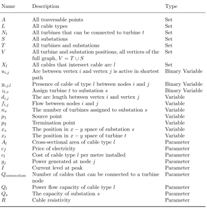
observed in figure 1. Though this could be avoided by using a finer grid size, other 272
challenges still remained. For example, by creating a grid, the cable paths were limited 273
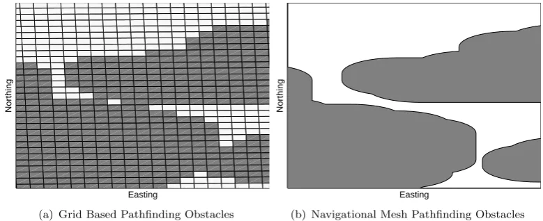
in having only 8 options of where to go from any given grid position (fig. 2), often causing 274
problems with paths overlapping cables near substations and no simple means of avoiding 275
this. Paths based on the grid were also longer than necessary due to being fixed to the 276
grid.
Easting
Northing
(a) Grid Based Pathfinding Obstacles
Easting
Northing
[image:9.595.107.497.183.342.2](b) Navigational Mesh Pathfinding Obstacles Figure 1. Comparison of obstacle representation in grid based and navigational mesh based pathfinding. 277
The alternative method uses what is known as a visibility graph and navigational 278
mesh, and is capable of avoiding all of the above problems, but at a significant cost in 279
complexity (Ghosh 2007). The visibility graph is a graph for which an arc exists between 280
any two vertices if they are ‘visible’ to one another. Visibility is defined as true if the 281
two points can be connected by an arc without the arc passing through an obstacle. 282
It is important to note that in terms of a visibility graph, points along the obstacle 283
edges are considered to be an open set, that is that valid arcs can pass along edges. 284
The optimal path is in fact the shortest path between vertices on such a graph. The 285
difficulty in working with visibility graphs is that algorithms for testing visibility are 286
computationally complex. The most efficient algorithms still operate in O(nlogn+k) 287
where n is the number of vertices and k is the number of edges (de Berg et al. 2008). 288
Given that the GIS constraints for a typical offshore wind farm will constitute several 289
thousand vertices this was thought to be too computationally complex. 290
The proposed methodology, therefore uses a heuristic algorithm which can create a close 291
approximation of the visibility graph in a fraction of the computational time. This ap-292
proach, known as a navigational mesh based pathfinding algorithm creates a traversable 293
graph which obeys the obstacle constraints. One such algorithm, proposed by Jan et al. 294
(2012, 2014) was adopted for this project. This approximation method uses the edges of 295
a constrained Delaunay Triangulation to define the graph. A Delaunay Triangulation is 296
defined as a triangulation in which no vertex is within the circumcircle of any triangle of 297
the triangulation, and a constrained Delaunay Triangulation is given the obstacle edges 298
as a constraint such that no triangulation edges cross the obstacles. By triangulating 299
the obstacle vertices along with the origin and destination positions it is possible to cre-300
ate a graph representing the traversable area. In order to improve the performance of 301
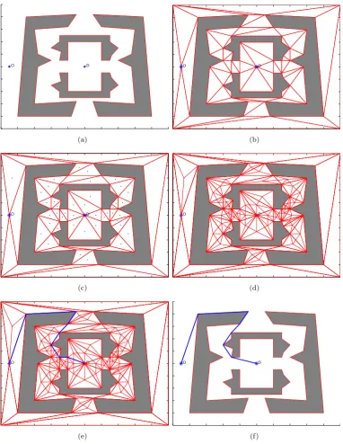
the graph and better approach the full visibility graph solution, this method includes the 302
Figure 2. Grid based system allows a path to go only to one of the 8 adjacent squares surrounding it. for triangles for which the largest angle is less than 120◦ to be the position internal to 304
the triangle that minimizes the distance to the triangle vertices. For a triangle in which 305
the largest angle is greater than or equal to 120◦ the Fermat point is located at one of 306
the vertices. Once these Fermat points are found, they are then added to the graph and 307
connected to their respective triangle vertices and any adjacent Fermat points (fig. 3(d) 308
and fig. 3(e)). 309
Algorithm 3 Delaunay Triangulation Based Navigational Mesh Shortest Path Require: Polygon obstacles, origin point, destination point, and site boundary
1: Construct the configurational space given the obstacle polygons
2: For the configurational map construct a constrained Delaunay triangulation for the vertices making up the obstacles, the origin point, and the destination point. The edges of the obstacles serve as the constraints for the triangulation.
3: Create a graph of all vertices and triangle edges of the triangulation 4: Insert Fermat points in triangles that have angles less than 120◦
5: Connect the Fermat points to the vertices of their triangles and any adjacent Fermat points
6: Find the shortest path in the graph using Dijkstra’s algorithm. 7: Apply the path shortening procedure
8: return Cable path
As this produces a potentially sub-optimal path, Jan et al. (2014) proposed a path
310
shortening method which removes redundant Fermat points or vertices from the solution
311
paths therefore reducing the total length to on average within 2% of the optimal path, 312
but in a fraction of the time. The original path shortening algorithm was enhanced 313
by checking all possible short-cuts, constructing a graph, and then running Dijkstra’s 314
shortest path algorithm. 315
Figure 3 shows a visual representation of the pathfinding process. Comparing the re-316
sulting paths in figures 3(e) and 3(f) shows the need for including the path shortening 317
subroutine. It is important to note that inclusion of the path-shortening algorithm with 318
the improvement suggested still does not ensure optimality, however, it can lead to sig-319
Algorithm 4 Path Shortening
Require: Polygon obstacles, cable path
1: Compute the length of each segment of the path 2: Compute the length for all possible shortcuts 3: for all possible shortcutsdo
4: if shortcut does not intersects an obstacle then 5: Add shortcut length to graph adjacency matrix 6: end if
7: end for
8: Find shortest path along graph using Dijkstra’s algorithm 9: return Cable path
does find the optimal path between two points. 321
5. MILP Formulation of Offshore Wind Farm Electrical Layout 322
Optimization 323
5.1 Problem Description
324
Through the preceding sub-problems the substations have been placed and a graph of 325
possible cable connections has been constructed with the path and length of each cable 326
computed. The remaining task is to select which of these cables to use to minimize the 327
total cost of the inter-array cable infrastructure. Given the arc costs between turbines 328
and the constraints described below, this problem could be described as a capacitated 329
minimum spanning tree (CMST) problem with additional constraints. The minimum 330
spanning tree problem (MST) seeks to find the sub-graph of a connected graph which 331
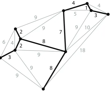
connects all vertices at minimum total cost (fig. 4). The CMST variation on this problem 332
introduces additional constraints to account for maximum capacities on the arcs. The 333
CMST is an NP-complete problem and exact methods are often avoided though easily 334
formulated. Similar to previous studies, the CMST was here implemented as an MILP 335
problem and solved using the Gurobi package through MATLAB. 336
The CMST is not a new problem and the formulation used in this work is based on 337
that of Gouveia (1993, 1995). This work has generalized this formulation to allow for 338
multiple arc types and a simultaneous selection of not only the cable paths, but the 339
O D
(a)
O D
(b)
O D
(c)
O D
(d)
O D
(e)
O D
(f)
[image:12.595.109.492.48.543.2]8 3
8 7
2 2
4
[image:13.595.203.397.52.215.2]3 1
Figure 4. Example of a minimum spanning tree with arc costs shown. 5.2 Problem Formulation
341
Mathematically, the CMST can be formulated as:
minimize X i∈V
X j∈N
X l∈L
(cl·di,j·yi,j,l) +
fi,j·yi,j,l·di,j ·
R
Al
·cf ·I2
(3a)
subject to X i∈V
X l∈L
yj,i,l ≤1 ∀j ∈V, (3b)
X i∈V
X l∈L
fj,i·yj,i,l− X i∈N
X l∈L
fi,j·yi,j,l =gj ∀j∈V, (3c)
fi,j−
X l∈L
Ql·yi,j,l≤0 ∀(i, j)∈V,∀l∈L, (3d)
X l∈L
yi,j,l≤1 ∀(i, j)∈V, (3e)
X l∈L
yi,j,l+yq,r,l ≤1 ∀(i, j, q, r)∈X, (3f)
X i∈V
X l∈L
yi,j,l+yj,i,l ≤Qconnection ∀j∈T, (3g)
fi,j ≥0 ∀(i, j)∈V, (3h)
yi,j,l ∈ {0,1} ∀(i, j)∈V,∀l∈L (3i)
The above formulation represents the minimum constraints to account for a CMST 342
with multiple arc types each with a different capacity ratings. In this formulation there 343
are two decision variables: fi,j represents the the power flow between nodes iand j and 344
yi,j,l is a binary variable representing the presence of a cable between nodes i and j of 345
cable-type l. Both i and j are turbine or substation elements of the set V and l is a 346
cable-type of the set L. The quantity Qconnection represents the physical constraint on 347
the number of connections at each turbine position. 348
The objective function is made up of two terms, the first represents the fixed capital 349
cost of the cable and its installation whereclis the per-length cost of cable-type l,di,j is 350
the length of cable needed between nodes i and j. The second term represents a factor 351
minimizes both the CAPEX costs of the cable and the losses in the cable. The losses 353
are monetized by applying a cost of electricity cf to represent the forgone revenue due 354
to the loss. The losses are computed using: R is the resistivity of the cable, Al is the 355
cross-sectional area of cable type l, andI is the current level at peak, the cable length, 356
and the flow in the cable. This bi-objective approach ensures that not only is the cable 357
length minimized, but solutions with lower flow levels in cables are preferred in order to 358
reduce Ohmic losses. 359
The seven constraints listed represent the minimum necessary for this problem includ-360
ing the fact that cables cannot cross one another. General CMST formulations and past 361
wind farm planning tools do not include the constraints given by eqs. (3e) to (3g) (Gou-362
veia 1993; Gavish 1983; Uchoa, Fukasawa, and Lysgaard 2006; Fagerfj¨all 2010; Svendsen 363
2013). Constraint 3b stipulates that each node, or turbine can have at most one cable 364
exporting power. Constraint 3c imposes the flow balance constraints such that the dif-365
ference between all flow out of each node and the flow into each node must be equal 366
to the flow supplied at each node (the power generated by the turbine) denoted by gj. 367
Constraint 3d imposes the capacity constraint where Ql is the capacity of cable-typel. 368
Constraint 3e ensures that every cable can be of only a single cable-type. Constraint 3f 369
accounts for the fact that for an offshore wind farm inter-array cables may not cross. In 370
order to impose this, X is the set of turbine pairs for which cables cross. Constraint 3g 371
constrains the number of cables connected to a turbine to Qconnection to account for the 372
physical space for circuit breakers in a turbine tower. Finally eqs. (3h) and (3i) constrain 373
xij to be a positive flow, and yijl to be a binary variable as explained earlier. 374
5.3 Solution Approach
375
Though previous work formulated the problem similarly, they identified that a heuristic 376
algorithm would be appropriate given the NP-completeness of the problem (Svendsen 377
2013; Lindahl et al. 2013; Li, He, and Fu 2008). For this reason it was decided to use 378
Gurobi 5.6, a commercial MILP solver which combines simplex solving techniques with 379
bespoke cutting plane generation algorithms, and heuristic algorithms. Using Gurobi, 380
the MIP gap, the relative difference between the upper and lower bounds, is used as 381
a measure of optimality and a termination criteria. Generally Gurobi attempts to find 382
a true global optimum which has an MIP gap approaching 0. In order to improve the 383
performance the MIP gap was relaxed to 0.01. This means that once the upper and lower 384
bound of the solutions are within a 1% difference the solution is considered optimal. This 385
means in the worst case, the solution found is 1% away from optimality for the given 386
path lengths. 387
Table 2. Comparison of full crossing constraint implementation to row generation method.
Number of Crossing Constraints Time to Solve CMST [s] Turbines Full Row Generation Full Row Generation
52 790804 104 701.47 1867.68
62 844914 2 847.94 13.79
61 405862 0 1340.13 36.43
Total 175 2041580 106 2889.54 1917.9
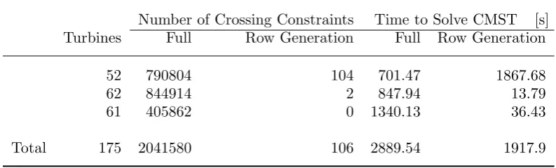
As stated earlier, the crossing constraints were imposed, however, it was found during 388
[image:14.595.100.497.559.679.2]for all pairs of cables resulted in many inactive constraints. It was also found that for 390
problems with more than 40 turbines significant amounts of memory were required in 391
order to avoid out of memory errors. It was instead decided to take an approach similar 392
to the implementation of cutting planes and instead solve the MILP, check if any of the 393
paths in the solution crossed, and if so impose that specific constraint. In this way the 394
MILP solver is called iteratively, slowly increasing the number of constraints, until the 395
solution is found. By doing this, the inactive constraints are not unnecessarily formulated 396
and less memory is required. Even in small cases this row generation approach was 397
shown to perform better than the full implementation. Table 2 shows a comparison of 398
the performance using the full constraints and using the row generation approach. Due to 399
the way in which the cable routes were found using the pathfinding algorithm described 400
in section 4 it was not necessary to impose further constraints representing the regions 401
where cables could not be placed. 402
Based on previous work by Fagerfj¨all (2010) it was decided to explore the introduction of additional constraints in order to improve performance. Two additional constraints were therefore introduced:
fi,j−
X l∈L
yi,j,l ≥0 ∀i, j∈T, (4a)
X i∈T
X l∈L
yi,j,l+yj,i,l ≥1 ∀j∈T (4b)
Equation 4a relates the flow and activity of an arc, while equation 4b stipulates that 403
there must be at least one active edge connected to each node. Neither of these constraints 404
is necessary in order to solve the problem, however, performance improvements were 405
noted when they were included. 406
6. Results 407
6.1 Study Description
408
In order to assess the performance of this approach compared to other MILP and simple 409
estimation methodologies it was applied for a real offshore wind farm. Navitus Bay 410
Windpark, off the south coast of England is a Round 3 wind farm site which will have 411
between 121 and 194 turbines. The site interestingly has a number of GIS constraints that 412
would need to be taken into account during both the siting of turbines and the design of 413
the inter-array cable network. These GIS constraints include unexploded World War II 414
ordnance (UXOs), ship wrecks, and areas where the seabed characteristics are unsuitable 415
for turbines or cables. 416
As no decision has been made on the layout of the turbines or the size of the turbine, 417
a realistic turbine layout was designed using WindFarmer 5.2. This layout considers 418
only the overall site boundary and the GIS constraints and has been generated for the 419
explicit purpose of testing this inter-array cable optimization tool; it does not represent 420
a real layout designed by the project developer. The layout studied here consists of 175 421
6 MW turbines representing 1050 MW installed. This layout is larger than the 968 MW 422
maximum allowed capacity for the wind farm and has been generated for the explicit 423
purpose of demonstrating the capabilities of this optimization tool. 424
For this layout, the results using this tool are compared to running a simple design 425
tool ignoring the GIS constraints, as well as estimating the total cable length only using 426
the separation distance between turbines in the crosswind direction. The latter two rep-427
estimation based on the turbine separation considers neither the GIS constraints nor the 429
capacity of cables and therefore represents a theoretical lower bound on the length of 430
cable. 431
! !
!
!
! !
! !
! !
!
The Needles Poole
Swanage
Yarmouth Weymouth
Bournemouth
Isle of Wight
Durlston Head
Barton on Sea
Milford on Sea
St Catherine’s Point Chirstchurch
Contains Ordnance Survey data © Crown copyright and database right 2013; NOT FOR NAVIGATIONAL USE
0
.
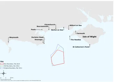
5 10kmKey
[image:16.595.110.492.107.382.2]New Boundary, Feb 2014 Old Boundary, Dec 2012 Original Boundary, Mar 2011
Figure 5. Illustrative map showing the Navitus Bay project site. Image courtesy Navitus Bay Development. Based on the most recent boundaries shown in figure 5 along with the GIS data pro-432
vided by the Navitus Bay Development it was possible to generate turbine layouts using 433
DNV GL WindFarmer 5.2. These turbine positions were then input to the inter-array 434
cable optimization tool. 435
All MILP optimization problems were run using a gap of 0.01. A solution is also shown 436
using the grid based pathfinding, however, this method required the relaxation of the 437
crossing constraint and the solutions produced by this method therefore do not represent 438
realistic solutions. 439
6.2 Substation Placement
440
Running first the substation placement component of the tool allowed the new con-441
strained capacitated kmeans++ (CC-kmeans++) algorithm to be benchmarked against 442
common clustering approaches such as traditional kmeans and kmeans++. It should be 443
noted that neither of these algorithms are designed to include capacity constraints or GIS 444
based constraints limiting the area where it is permissible to place the cluster center. 445
Comparing the performance for a range of wind farm sizes within the Navitus Bay 446
region it was found that the clustering was relatively inelastic to the number of turbines, 447
and more strongly governed by the number of clusters that the turbines were to be 448
partitioned into. Importantly, the constrained capacitated kmeans++ approach proved 449
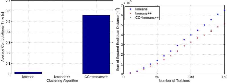
to be far slower than traditional clustering approaches, however, even given this it was 450
two clusters in less than a second. 452
As can be seen in figure 6 though the performance of the new clustering algorithm is 453
much slower than kmeans++, it gives similar results in terms of total distance between 454
the turbines and the center location while at the same time adhering to the GIS and 455
substation capacity constraints. Though the increase in computational time is relatively 456
significant it is still a quick algorithm in absolute terms partitioning 150 turbines into 457
two clusters in under 0.6 seconds. 458
kmeans kmeans++ CC−kmeans++ 0
0.1 0.2 0.3 0.4 0.5 0.6 0.7
Clustering Algorithm
Average Computational Time [s]
(a) Average time to partition wind farm into two clus-ters.
0 50 100 150
0 1 2 3 4 5 6 7x 10
5
Number of Turbines
Sum of Squared Euclidean Distance [m
2] kmeans kmeans++ CC−kmeans++
(b) Sum of distance between turbines and substation. Figure 6. Comparison of the clustering algorithms. In both graphs lower values indicate better performance.
6.3 Optimized Inter-Array Cable Layout
459
The full implementation of both the substation placement and the inter-array cable 460
optimization for a number of wind farms within the Navitus Bay site area gave the 461
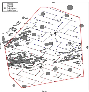
cable results shown in figures 7 and 8. When compared to the solutions of simpler MILP 462
programmes, ignoring GIS constraints, it was found that the total cable length increased 463
by almost 9 km representing an added capital cost of approximately e4.5 million and 464
when compared to using an estimation based on the inter-turbine spacing, the total 465
amount of cable is increased by approximately 13 km representing approximately e6.5 466
million. 467
Table 3. Cable Length Comparison
Method Cable Length [km] Delta [km]
Turbine Spacing Based 148.75
-CMST no GIS 157.66 8.91
CMST with GIS 161.84 13.09
From the results, a number of differences can be observed; ignoring the GIS constraints 468
leads to a number of cables crossing the obstacle regions as would be expected. Interest-469
ingly, however, running either the A* grid based pathfinding (fig. 9) or the navigational 470
mesh both produce fundamentally different solutions to the cable layout problem from 471
the base case. This can be attributed to the optimal solution being more than just re-472
[image:17.595.100.499.154.301.2] [image:17.595.148.454.546.621.2]Easting
Northing
[image:18.595.145.458.42.363.2]Phase1 Phase2 Substations Cable Type 1
Figure 7. Cable layout, no GIS constraints.
Looking at the A* solution shown in figure 9, it can be observed that the grid based 474
system experiences difficulty due to the limitations mentioned previously and in fact 475
was unable to produce solutions without cables crossing. The proposed full methodology 476
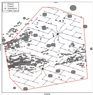
does, however, successfully place the substations at acceptable locations and designs an 477
infield cable layout that does not violate any of the constraints including the GIS based 478
constraints. This is shown in figure 8. 479
7. Conclusion 480
This article has outlined a new approach for the inter-array cable design problem for an 481
offshore wind farm by means of breaking it into several sub-problems. These sub-problems 482
have included a location-constrained capacitated clustering approach for placing the sub-483
stations, a navigational mesh based pathfinding algorithm to determine possible cable 484
connections, and a MILP approach to solve for a CMST and select which cable connec-485
tions should be installed. 486
The CCCP compares well in performance against traditional clustering methods such 487
as kmeans and kmeans++, though consistently slower than both, it has consistently bet-488
ter cluster centres than kmeans, and very similar results to kmeans++ while respecting 489
the GIS constraints. This implementation represents a novel approach to the position-490
ing of an offshore substation and is one of the first automated approaches used for this 491
application. 492
This study then opted to implement a navigational mesh pathfinding algorithm to 493
determine possible cable connections based on constructing an approximation of a vis-494
Easting
Northing
[image:19.595.145.458.42.364.2]Phase1 Phase2 Substations Cable Type 1
Figure 8. Cable layout, full optimization method.
the resulting graph that is constructed a simple shortest path algorithm with a bespoke 496
path shortening heuristic is applied in order to produce good feasible solutions which 497
approach optimality. The lengths of these paths are then used as edge lengths in an 498
MILP implementation of a capacitated minimum spanning tree. 499
The results of this approach applied to a real offshore wind farm currently in the 500
planning stages have yielded promising results indicating that this approach is not only 501
valid but shows improvements over commonly used approaches based on the turbine 502
separation distance. There are, still improvements that can be made, but this approach 503
represents a strong step forward to the efficient automation of the layout design of an 504
offshore wind farm and optimizing all aspects of the layout. 505
Acknowledgements 506
The authors would like to acknowledge EDF Energy Renewables and the Navitus Bay 507
Project Development teams for the provision of the Navitus Bay GIS data and maps of 508
the site. 509
This work is funded in part by the ETI and RCUK Energy programme for IDCORE 510
Easting
Northing
[image:20.595.147.459.48.366.2]Phase1 Phase2 Substations Cable Type 1
References 512
Arthur, David, and Sergei Vassilvitskii. 2006. k-means ++ : The Advantages of Careful Seeding. 513
Tech. rep.. Stanford InfoLab. 514
Bauer, J, and J Lysgaard. 2013. “The Offshore Wind Farm Array Cable Layout ProblemA Planar 515
Open Vehicle Routing Problem.”ii.uib.no 1–16. 516
Burton, T, N Jenkins, D Sharpe, and E Bossanyi. 2011. Wind energy handbook. 2nd ed. John 517
Wiley & Sons, Ltd. 518
Cerveira, Adelaide, and Eduardo J Solteiro Pires. 2014. “Optimisation Design in Wind Farm 519
Distribution Network.” Proceedings of International Joing Conference
SOCO’13-CISIS’13-520
ICEUTE’13, Advances in Intelligent Systems and Computing 239. 521
Chamorro, Leonardo P., and Fernando Port´e-Agel. 2010. “Effects of Thermal Stability and Incom-522
ing Boundary-Layer Flow Characteristics on Wind-Turbine Wakes: A Wind-Tunnel Study.” 523
Boundary-Layer Meteorology 136 (3): 515–533. 524
Chaves, Antonio Augusto, and Luiz Antonio Nogueira Lorena. 2010. “Clustering search algorithm 525
for the capacitated centered clustering problem.” Computers & Operations Research 37 (3): 526
552–558. 527
de Berg, Mark, Otfried Cheong, Marc van Kreveld, and Marc Overmars. 2008. Computational
528
Geometry. 3rd ed. Berlin, Heidelberg: Springer-Verlag. 529
Dutta, S, and TJ Overbye. 2011. “A clustering based wind farm collector system cable layout 530
design.”Power and Energy Conference at Illinois (PECI)4–9. 531
Dutta, Sudipta, and Thomas Overbye. 2013. “A graph-theoretic approach for addressing trenching 532
constraints in wind farm collector system design.”2013 IEEE Power and Energy Conference
533
at Illinois (PECI)48–52. 534
Dutta, Sudipta, and Thomas J Overbye. 2012. “Design Considering Total Trenching Length.” 535
IEEE Transactions on Sustainable Energy 3 (3): 339–348. 536
Elkinton, Christopher Neil. 2007. “Offshore Wind Farm Layout Optimization.” Doctor of philos-537
ophy. University of Massachussetts Amherst. 538
Fagerfj¨all, Patrik. 2010. “Optimizing wind farm layout more bang for the buck using mixed inte-539
ger linear programming.” Master of science. Chalmers University of Technology and Gothen-540
burgh University. 541
Gavish, Bezalel. 1983. “Formulations and Algorithms for the Capacitated Minimal Directed Tree 542
Problem.”Journal of the ACM 30 (1): 118–132. 543
Geetha, S, G Poonthalir, and PT Vanathi. 2009. “Improved K-Means Algorithm for Capacitated 544
Clustering Problem.”International INFOCOMP Journal of Computer Science . 545
Ghosh, SK. 2007. Visibility algorithms in the plane. 1st ed. Cambridge: Cambridge University 546
Press. 547
Gonz´alez-Longatt, FM, and Peter Wall. 2012. “Optimal electric network design for a large offshore 548
wind farm based on a modified genetic algorithm approach.”IEEE Systems Journal 6 (1): 164– 549
172. 550
Gouveia, L. 1993. “A comparison of directed formulations for the capacitated minimal spanning 551
tree problem.”Telecommunication Systems 1: 51–76. 552
Gouveia, Luis. 1995. “A 2n Constraint Formulation for the Capacitated Minimal Spanning Tree 553
Problem.”Operations Research 43 (1): 130–141. 554
Jan, Gene Eu, Chi-chia Sun, Wei Chun Tsai, and Ting-hsiang Lin. 2014. “An O (n log n ) 555
Shortest Path Algorithm Based on Delaunay Triangulation.” IEEE/ASME Transactions on
556
Mechatronics 19 (2): 660–666. 557
Jan, Gene Eu, Wei Chun Tsai, Chi-Chia Sun, and Bor-Shing Lin. 2012. “A Delaunay 558
triangulation-based shortest path algorithm with O(n log n) time in the Euclidean plane.”2012
559
IEEE/ASME International Conference on Advanced Intelligent Mechatronics (AIM)186–189. 560
Li, DD, Chao He, and Yang Fu. 2008. “Optimization of internal electric connection system of 561
large offshore wind farm with hybrid genetic and immune algorithm.”Conference Proceedings
562
DRPT (April): 2476–2481. 563
Lindahl, M., N.C. Fink Bagger, T. Stidsen, S. Frost Ahrenfeldt, and I. Arana. 2013. “OptiArray 564
from DONG Energy.”Proceedings of Wind Integration Workshop . 565
wind farm applying decomposition strategies.”IEEE Transactions on Power Systems 28 (2): 567
1434–1441. 568
MacQueen, J. 1967. “Some methods for classification and analysis of multivariate observations.” 569
Proceedings of the fifth Berkeley symposium on Mathematical Statistics and Probability 233 570
(233): 281–297. 571
Negreiros, Marcos, and Augusto Palhano. 2006. “The capacitated centred clustering problem.” 572
Computers & Operations Research 33 (6): 1639–1663. 573
Svendsen, Harald G. 2013. “Planning Tool for Clustering and Optimised Grid Connection of 574
Offshore Wind Farms.”Energy Procedia 35: 297–306. 575
Uchoa, Eduardo, Ricardo Fukasawa, and Jens Lysgaard. 2006. “Robust branch-cut-and-price for 576
the capacitated minimum spanning tree problem over a large extended formulation.”
Mathe-577
matical Programming 1–30. 578
Zhao, M, Z Chen, and F Blaabjerg. 2008. “Application of genetic algorithm in electrical system 579
optimization for offshore wind farms.”. . . and Power . . . (April): 7–12. 580
Zhao, M, Z Chen, and F Blaabjerg. 2009. “Optimisation of electrical system for offshore wind 581