
Ivan Markovsky∗,1and Sabine Van Huffel2
1 — School of Electronics and Computer Science, University of Southampton, SO17 1BJ, UK,[email protected]
2 — Katholieke Universiteit Leuven, ESAT-SCD/SISTA, Kasteelpark Arenberg 10 B–3001 Leuven, Belgium,[email protected]
Abstract
We review the development and extensions of the classical total least squares method and describe algorithms for its generalization to weighted and structured approximation problems. In the generic case, the classical total least squares problem has a unique solution, which is given in analytic form in terms of the singular value de-composition of the data matrix. The weighted and structured total least squares problems have no such analytic solution and are currently solved numerically by local optimization methods. We explain how special structure of the weight matrix and the data matrix can be exploited for efficient cost function and first derivative computation. This allows to obtain computationally efficient solution methods. The total least squares family of methods has a wide range of applications in system theory, signal processing, and computer algebra. We describe the applications for deconvolution, linear prediction, and errors-in-variables system identification.
Keywords: Total least squares; Orthogonal regression; Errors-in-variables model; Deconvolution; Linear
pre-diction; System identification.
1
Introduction
The total least squares method was introduced by Golub and Van Loan [25, 27] as a solution technique for an overde-termined system of equations AX≈B, where A∈Rm×nand B∈Rm×dare the given data and X ∈Rn×d is unknown. With m>n, typically there is no exact solution for X , so that an approximate one is sought for. The total least squares method is a natural generalization of the least squares approximation method when the data in both A and B is perturbed.
The least squares approximationXblsis obtained as a solution of the optimization problem
{Xbls,∆Bls}:=arg min
X,∆Bk∆BkF subject to AX=B+∆B. (LS) The rationale behind this approximation method is to correct the right-hand side B as little as possible in the Frobenius norm sense, so that the corrected system of equations AX=B,b B :b =B+∆B has an exact solution. Under the condition that A is full column rank, the unique solution Xbls= (A⊤A)−1A⊤B of the optimally corrected system of equations
AX=Bbls,Bbls:=B+∆Blsis by definition the least squares approximate solution of the original incompatible system of equations.
The definition of the total least squares method is motivated by the asymmetry of the least squares method: B is corrected while A is not. Provided that both A and B are given data, it is reasonable to treat them symmetrically. The classical total least squares problem looks for the minimal (in the Frobenius norm sense) corrections∆A and ∆B on the given data A and B that make the corrected system of equationsAXb =B,b A :b =A+∆A,B :b =B+∆B solvable, i.e.,
{Xbtls,∆Atls,∆Btls}:=arg min X,∆A,∆B
∆A ∆BF subject to (A+∆A)X=B+∆B. (TLS1)
∗Corresponding author.
The total least squares approximate solutionXbtls for X is a solution of the optimally corrected system of equations b
AtlsX =Bbtls,Abtls:=A+∆Atls,Bbtls:=B+∆Btls.
The least squares approximation is statistically motivated as a maximum likelihood estimator in a linear regression model under standard assumptions (zero mean, normally distributed residual with a covariance matrix that is a multiple of the identity). Similarly, the total least squares approximation is a maximum likelihood estimator in the errors-in-variables model
A=A¯+A˜, B=B¯+B˜, there exists an ¯X∈Rn×d such that ¯A ¯X =B¯ (EIV) under the assumption that vec(A˜ B˜)is a zero mean, normally distributed random vector with a covariance matrix that is a multiple of the identity. In the errors-in-variables model, ¯A, ¯B are the “true data”, ¯X is the “true” value of the parameter X , and ˜A, ˜B consist of “measurement noise”.
Our first aim is to review the development and generalizations of the total least squares method. We start in Section 2 with an overview of the classical total least squares method. Section 2.1 gives historical notes that relate the total least squares method to work on consistent estimation in the errors-in-variables model. Section 2.2 presents the solution of the total least squares problem and the resulting basic computational algorithm. Some properties, generalizations, and applications of the total least squares method are stated in Sections 2.3, 2.4, and 2.5.
Our second aim is to present an alternative formulation of the total least squares problem as a matrix low rank approximation problem
b
Ctls:=arg min
b
C k
C−CbkF subject to rank(Cb)≤n, (TLS2) which in some respects, described in detail later, has advantages over the classical one. With C=A B, the classical total least squares problem (TLS1) is generically equivalent to the matrix low rank approximation problem (TLS2), however, in certain exceptional cases, known in the literature as non-generic total least squares problems, (TLS1) fails to have a solution, while (TLS2) always has a solution.
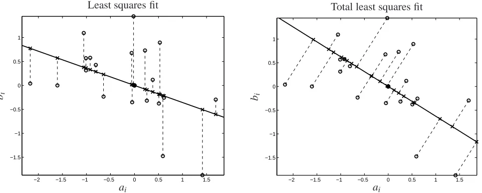
The following example illustrates the geometry behind the least squares and total least squares approximations.
Example 1 (Geometry of the least squares and total least squares methods). Consider a data matrix C=a bwith m=20 rows and n+d=2 columns. The data is visualized in the plane: the rowsai bi
of C correspond to the circles on Figure 1. Finding an approximate solutionbx of the incompatible system of equations ax≈b amounts to fitting the data points by a non-vertical line passing through the origin. (The vertical line can not be represented by an x∈R). The cases when the best fitting line happens to be vertical correspond to non-generic problems.
Alternatively, finding a rank-1 approximationC of the given matrix C (refer to problem (TLS2)) amounts to fittingb the data points ai bi
by points habi bbi i
(corresponding to the rows ofC) that lie on a line passing through theb origin. Note that now we do not exclude an approximation by the vertical line, because approximation points lying on a vertical line define a rank deficient matrixC and problem (TLS2) does not impose further restrictions on theb solution.
The least squares and total least squares methods assess the fitting accuracy in different ways: the least squares method minimizes the sum of the squared vertical distances from the data points to the fitting line, while the total least squares method minimizes the sum of the squared orthogonal distances from the data points to the fitting line. Figure 1 shows the least squares and total least squares fitting lines as well as the data approximation (the crosses lying on the lines). In the least squares case, the data approximationCbls=a b+∆blsis obtained by correcting the second coordinate only. In the total least squares case, the data approximationCbtls=
a+∆atls b+∆btls
is obtained by correcting both coordinates.
In (TLS1) the constraintAXb =B represents the rank constraint rankb (Cb)≤n, via the implication there exists an X ∈Rn×dsuch thatAXb =Bb =⇒ C :b =hAb Bb
i
, rank(Cb)≤n.
−2 −1.5 −1 −0.5 0 0.5 1 1.5 −1.5
−1 −0.5 0 0.5 1
ai bi
Least squares fit
−2 −1.5 −1 −0.5 0 0.5 1 1.5 −1.5
−1 −0.5 0 0.5 1
ai bi
[image:3.595.57.540.61.255.2]Total least squares fit
Figure 1: Least squares and total least squares fits of a set of m=20 data points in the plane.◦—data pointsai bi
,
×—approximations habi bbi i
, solid line—fitting modelbabx=bb, dashed lines—approximation errors.
Apart fromAXb =B withb Cb=hAb Bb i
, there are numerous other ways to represent the rank constraint rank(Cb)≤n. For example,AXb =B withb CbΠ=hAb Bb
i
, whereΠis an arbitrary permutation matrix, i.e., in (TLS2) we can choose to
express any d columns ofC as a linear combination of the remaining columns in order to ensure rank deficiency ofb C.b Any a priori fixed selection, however, leads to non-generic problems and therefore will be inadequate in certain cases. Of special importance are the kernel representation RCb⊤=0, where RR⊤=Id, and the image representationCb⊤=PL, where P∈R(n+d)×n, L∈Rn×m. In contrast to the input/output representations, the kernel and image representations are equivalent to rank(Cb)≤n.
The representation-free total least squares problem formulation (TLS2), described in Section 3, is inspired by the behavioral approach to system theory, put forward by J. C. Willems in the three part remarkable paper [91]. We give an interpretation of the abstract rank condition as existence of a linear static model for the given data. Then
the total least squares method is viewed as a tool for deriving approximate linear static models.
This point of view is treated in more details for dynamic as well as static models in [51].
Notation
RandR+ the set of real numbers and nonnegative real numbers :=and :⇐⇒ left-hand side is defined by the right-hand side =: and ⇐⇒: right-hand side is defined by the left-hand side vec column-wise vectorization of a matrix
C,∆C,Cb data, correction, and approximation matrices C=A B input/output partitioning of the data
c1, . . . ,cm observations,
c1 ··· cm
=C⊤ c=col(a,b) the column vector c= [a
b]
B⊆Rn+d a static model inRn+d L linear static model class
B∈Ln linear static model of dimension at most n, i.e.,
a subspace (inRn+d) of dimension at most n
X , R, P parameters of input/output, kernel, and image representations
Bi/o(X) input/output representation, see (I/O repr) on page 9
col span(P) image representation, i.e., the space spanned by the columns of P ker(R) kernel representation, i.e., the right null space of R
2
The classical total least squares method
2.1 History
Although the name “total least squares” appeared only recently in the literature [25, 27], this fitting method is not new and has a long history in the statistical literature where it is known as “orthogonal regression”, “errors-in-variables”, and “measurement errors”. The univariate (n=1, d =1) problem is discussed already in 1877 by Adcock [2]. Latter on contributions are made by Adcock [3], Pearson [62], Koopmans [30], Madansky [43], and York [94]. The orthogonal regression method has been rediscovered many times, often independently. About thirty years ago, the technique was extended by Sprent [76] and Gleser [24] to multivariate (n>1, d>1) problems.
More recently, the total least squares method also stimulated interest outside statistics. In the field of numerical analysis, this problem was first studied by Golub and Van Loan [25, 27]. Their analysis, as well as their algorithm, are based on the singular value decomposition. Geometrical insight into the properties of the singular value decomposition brought Staar [77] independently to the same concept. Van Huffel and Vandewalle [84] generalized the algorithm of Golub and Van Loan to all cases in which their algorithm fails to produce a solution, described the properties of these so-called non-generic total least squares problems and proved that the proposed generalization still satisfies the total least squares criteria if additional constraints are imposed on the solution space. This seemingly different linear algebraic approach is actually equivalent to the method of multivariate errors-in-variables regression analysis, studied by Gleser [24]. Gleser’s method is based on an eigenvalue-eigenvector analysis, while the total least squares method uses the singular value decomposition which is numerically more robust in the sense of algorithmic implementation. Furthermore, the total least squares algorithm computes the minimum norm solution whenever the total least squares solution is not unique. These extensions are not considered by Gleser.
total least squares and its relation to errors-in-variables modeling. The computational advantages of total least squares are still largely unknown in the statistical community, while inversely the concept of errors-in-variables modeling did not penetrate sufficiently well in the field of computational mathematics and engineering.
A comprehensive description of the state of the art on total least squares from its conception up to the summer of 1990 and its use in parameter estimation has been presented in Van Huffel and Vandewalle [87]. While the latter book is entirely devoted to total least squares, a second [81] and third [82] edited books present the progress in total least squares and in the field of errors-in-variables modeling respectively from 1990 till 1996 and from 1996 till 2001.
2.2 Algorithm
The following theorem gives conditions for the existence and uniqueness of a total least squares solution.
Theorem 2 (Solution of the classical total least squares problem). Let
C :=A B=UΣV⊤, where Σ=diag(σ1, . . . ,σn+d)
be a singular value decomposition of C,σ1≥ ··· ≥σn+d be the singular values of C, and define the partitionings
V :=
n d
V11 V12
V21 V22
n
d and Σ:=
n d
Σ
1 0
0 Σ2
n d .
A total least squares solution exists if and only if V22is non-singular. In addition, it is unique if and only ifσn6=σn+1. In the case when the total least squares solution exists and is unique, it is given by
b
Xtls=−V12V22−1 and the corresponding total least squares correction matrix is
∆Ctls:= ∆
Atls ∆Btls
=−U diag(0,Σ2)V⊤.
In the generic case when a unique total least squares solutionXbtls exists, it is computed from the d right singular vectors corresponding to the smallest singular values by normalization. This gives Algorithm 1 as a basic algorithm for solving the classical total least squares problem (TLS1). Note that the total least squares correction matrix∆Ctlsis such that the total least squares data approximation
b
Ctls:=C+∆Ctls=U diag(Σ1,0)V⊤ is the best rank-n approximation of C.
Algorithm 1 Basic total least squares algorithm. Input: A∈Rm×nand B∈Rm×d.
1: Compute the singular value decompositionA B=UΣV⊤.
2: if V22is nonsingular then
3: SetXbtls=−V12V22−1.
4: else
5: Output a message that the problem (TLS1) has no solution and stop.
6: end if
Output: Xbtls— a total least squares solution of AX≈B.
2.3 Properties
Consider the errors-in-variables model (EIV) and assume that vec(A˜ B˜) is a zero mean random vector with a multiple of the identity covariance matrix. In addition, assume that limm→∞A˜⊤A˜/m exists and is a positive definite
matrix. Under these assumptions it is proven [23, 25] that the total least squares solutionXbtls is a weakly consistent estimator of the true parameter values ¯X , i.e.,
b
Xtls→X in probability¯ as m→∞.
This total least squares property does not depend on the distribution of the errors. The total least squares correction ∆
Atls ∆Btls, however, being a rank d matrix is not an appropriate estimator for the measurement error matrix ˜
A B˜(which is a full rank matrix with probability one). Note that the least squares estimatorXblsis inconsistent in the errors-in-variables case.
In the special case of a single right hand side (d=1) and A full rank, the total least squares problem has an analytic expression that is similar to the one of the least squares solution
least squares: xbls= (A⊤A)−1A⊤b, total least squares: bxtls= (A⊤A−σn+12 I)−1A⊤b, (∗) whereσn+1is the smallest singular value ofA b. From a numerical analyst’s point of view, (∗) tells that the total least squares solution is more ill-conditioned than the least squares solution since it has a higher condition number. The implication is that errors in the data are more likely to affect the total least squares solution than the least squares solution. This is particularly true for the worst case perturbations. In fact, total least squares is a deregularizing procedure. However, from a statistician’s point of view, (∗) tells that the total least squares method asymptotically removes the bias by subtracting the error covariance matrix (estimated byσ2
n+1I) from the data covariance matrix A⊤A. While least squares minimizes a sum of squared residuals, total least squares minimizes a sum of weighted squared residuals:
least squares: min
x kAx−bk
2, total least squares: min x
kAx−bk2 kxk2+1 .
From a numerical analyst’s point of view, total least squares minimizes the Rayleigh quotient. From a statistician’s point of view, total least squares weights the residuals by multiplying them with the inverse of the corresponding error covariance matrix in order to derive a consistent estimate.
Other properties of total least squares, which were studied in the field of numerical analysis, are its sensitivity in the presence of errors on all data [87]. Differences between the least squares and total least squares solution are shown to increase when the ratio between the second smallest singular value ofA band the smallest singular value of A is growing. In particular, this is the case when the set of equations Ax≈b becomes less compatible, the vector y is growing in length, or A tends to be rank-deficient. Assuming independent and identically distributed errors, the improved accuracy of the total least squares solution compared to that of the least squares solution is maximal when the orthogonal projection of b is parallel to the singular vector of A corresponding to the smallest singular value. Additional algebraic connections and sensitivity properties of the total least squares and least squares problems, as well as other statistical properties have been described in [87, 81].
2.4 Extensions
The statistical model that corresponds to the basic total least squares approach is the errors-in-variables model with the restrictive condition that the measurement errors are zero mean independent and identically distributed. In order to relax these restrictions, several extensions of the total least squares problem have been investigated. The mixed least squares-total least squares problem formulation allows to extend consistency of the total least squares estimator in errors-in-variables models, where some of the variables are measured without error. The data least squares prob-lem [15] refers to the special case in which the A matrix is noisy and the B matrix is exact. When the errorsA˜ B˜ are row-wise independent with equal row covariance matrix (which is known up to a scaling factor), the generalized total least squares problem formulation [86] allows to extend consistency of the total least squares estimator.
Robustness of the total least squares solution is also improved by adding regularization, resulting in regularized total least squares methods [20, 26, 74, 73, 7]. In addition, various types of bounded uncertainties have been proposed in order to improve robustness of the estimators under various noise conditions [18, 11].
Similarly to the classical total least squares estimator, the generalized total least squares estimator is computed reliably using the singular value decomposition. This is no longer the case for more general weighted total least squares problems where the measurement errors are differently sized and/or correlated from row to row. Consistency of the weighted total least squares estimator is proven and an iterative procedure for its computation is proposed in [32]. This problem is discussed in more detail in Section 4.
Furthermore, constrained total least squares problems have been formulated. Arun [5] addressed the unitarily constrained total least squares problem, i.e., AX≈B, subject to the constraint that the solution matrix X is unitary. He proved that this solution is the same as the solution to the orthogonal Procrustes problem [28, page 582]. Abatzoglou et al. [1] considered yet another constrained total least squares problem, which extends the classical total least squares problem to the case where the errorsA˜ B˜are algebraically related. In this case, the total least squares solution is no longer statistically optimal (e.g., maximum likelihood in the case of normal distribution).
In the so-called structured total least squares problems [12], the data matrix A B is structured. In order to preserve the maximum likelihood properties of the solution, the total least squares problem formulation is ex-tended [31] with the additional constraint that the structure of the data matrixA Bis preserved in the correction matrix∆A ∆B. Similarly to the weighted total least squares problem, the structured total least squares solution, in general, has no closed form expression in terms of the singular value decomposition. An important exception is the circulant structured total least squares, which can be solved using the fast Fourier transform, see [6]. In the general case, a structured total least squares solution is searched via numerical optimization methods. However, efficient al-gorithms are proposed in the literature that exploit the matrix structure on the level of the computations. This research direction is further described in Section 5.
Regularized structured total least squares solution methods are proposed in [95, 56]. Regularization turns out to be important in the application of the structured total least squares method for image deblurring [57, 60, 59]. In addition, solution methods for nonlinearly structured total least squares methods are developed in [68, 40].
2.5 Applications
Since the publication of the singular value decomposition based total least squares algorithm [27], many new total least squares algorithms have been developed and, as a result, the number of applications in total least squares and errors-in-variables modeling has increased in the last decade. Total least squares is applied in computer vision [58], image reconstruction [65, 54, 22], speech and audio processing [39, 29], modal and spectral analysis [89, 93], linear system theory [14, 13], system identification [66, 37, 63, 52], and astronomy [8]. An overview of errors-in-variables methods in system identification is given by Söderström in [75]. In [81, 82], the use of total least squares and errors-in-variables models in the application fields are surveyed and new algorithms that apply the total least squares concept are described.
A lot of common problems in system identification and signal processing can be reduced to special types of block-Hankel and block-Toeplitz structured total least squares problems. In the field of signal processing, in particular in-vivo magnetic resonance spectroscopy, and audio coding, new state-space based methods have been derived by making use of the total least squares approach for spectral estimation with extensions to decimation and multichannel data quantification [35, 36]. In addition, it has been shown how to extend the least mean squares algorithm to the errors-in-variables context for use in adaptive signal processing and various noise environments. Finally, total least squares applications also emerge in other fields, including information retrieval [21], shape from moments [69], and computer algebra [96, 47].
3
Representation-free total least squares problem formulation
A subspaceB⊆Rn+d is referred to as a linear static model. Its dimension n is a measure of the model
complexity: the higher the dimension the more complex and therefore less useful is the modelB.
The set of all linear static models of dimension at most n is denoted byLn. It is a nonconvex set and has special
properties that make it a Grassman manifold. Letc1 ··· cm
:=C⊤, i.e., ciis the transposed ith row of the matrix C and define the shorthand notation
C∈B⊆Rn+d :⇐⇒ ci∈B, for i=1, . . . ,m.
We have the following equivalence
rank(C)≤n ⇐⇒ C∈B∈Ln,
which relates the total least squares problem (TLS2) to approximate linear static modeling. We restate problem (TLS2) with this new interpretation and notation.
Problem 3 (Total least squares). Given a data matrix C∈Rm×(n+d)and a complexity specification n, solve the opti-mization problem
{Bbtls,Cbtls}:=arg min
B∈LnCminb ∈Bk
C−CbkF. (TLS)
Note that (TLS) is a double minimization problem. On the inner level is the search for the best approximation of the given data C in a given modelB. The optimum value of this minimization
Mtls(C,B):=min
b
C∈Bk
C−CbkF (Mtls)
is a measure of the lack of fit between the data and the model and is called misfit. On the outer level is the search for the optimal model in the model classLn of linear static models with bounded complexity. The optimality of the
model is in terms of the total least squares misfit function Mtls.
The double minimization structure, described above, is characteristic for all total least squares problems. Since the modelB is linear and the cost function is convex quadratic, the inner minimization can be solved analytically
yielding a closed form expression for the misfit function. The resulting outer minimization, however, is a nonconvex optimization problem and needs numerical solution methods. In the case of the basic total least squares problem and the generalized total least squares problem, presented in Section 3.3, the outer minimization can be brought back to a singular value decomposition computation. In more general cases, however one has to rely on nonconvex optimization methods and the guarantee to compute a global solution quickly and efficiently is lost.
In order to solve numerically the abstract total least squares problem (TLS), we need to parameterize the fitting model. This important issue is discussed next.
3.1 Kernel, image, and input/output representations
As argued in the introduction, the representation-free formulation is conceptually useful. For analysis, however, often it is more convenient to consider concrete representations of the model, which turn the abstract problem (TLS) into concrete parameter optimization problems, such as (TLS1). In this section, we present three representations of a linear static model: kernel, image, and input/output. They give different parameterizations of the model and are important in setting up algorithms for the solution of the problem.
Kernel representation
LetB∈Ln, i.e.,B is an n-dimensional subspace ofRn+d. A kernel representation ofB is given by a system of
equations Rc=0, such that
B={c∈Rn+d |Rc=0}=: ker(R).
The matrix R∈Rg×(n+d)is a parameter of the modelB.
1. R might have redundant rows, and
2. for a full rank matrix U , ker(R) =ker(U R).
The parameter R having redundant rows is related to the minimality of the representation. For a given linear static modelB, the representation Rc=0 ofBis minimal if R has the minimal number of rows among all parameters R
that define a kernel representation ofB. The kernel representation, defined by R, is minimal if and only if R is full
row rank.
Because of item 2, a minimal kernel representation is still not unique. All minimal representations, however, are related to a given one via a pre-multiplication of the parameter R with a nonsingular matrix U . In a minimal kernel representation, the rows of R are a basis for B⊥, the orthogonal complement of B, i.e., B⊥=row span(R). The
choice of R is non-unique due to the non-uniqueness in the choice of basis ofB⊥.
The minimal number of independent linear equations necessary to define a linear static modelB is d, i.e., in a
minimal representationB=ker(R)with row dim(R) =d.
Image representation
The dual of the kernel representationB=ker(R)is the image representation B={c∈Rn+d |c=Pl,l∈Rl}=: col span(P).
Again for a givenB∈Lnan image representationB=col span(P)is not unique because of possible non-minimality
of P and the choice of basis. The representation is minimal if and only if P is a full column rank matrix. In a minimal image representation, col dim(P) =dim(B)and the columns of P form a basis forB. Clearly col span(P) =
col span(PU), for any nonsingular matrix U∈Rl×l. Note that
ker(R) =col span(P) =B∈Ln =⇒ RP=0,
which gives a link between the parameters P and R.
Input/output representation
Both, the kernel and the image representations, treat all variables on an equal footing. In contrast, the more classical input/output representation
Bi/o(X):={c=: col(a,b)∈Rn+d|X⊤a=b} (I/O repr)
distinguishes free variables a∈Rn, called inputs, and dependent variables b∈Rd, called outputs. In an input/output representation, a can be chosen freely, while b is fixed by a and the model. Note that for repeated observations C⊤=
c1 ··· cm
the statement C∈Bi/o(X)is equivalent to the linear system of equations AX=B, whereA B:=C
with A∈Rm×nand B∈Rm×d.
The partitioning c=col(a,b)gives an input/output partitioning of the variables: the first n :=dim(a)variables are inputs and the remaining d :=dim(b)variables are outputs. An input/output partitioning is not unique. Given a kernel or image representation, finding an input/output partitioning is equivalent to selecting a d×d full rank submatrix of R or an n×n full rank submatrix of P. In fact, generically, any splitting of the variables into a group of d variables (outputs) and a group of remaining variables (inputs), defines a valid input/output partitioning. In non-generic cases certain partitionings of the variables into inputs and outputs are not possible.
Note that in (I/O repr), the first n variables are fixed to be inputs, so that given X , the input/output representBi/o(X)
is fixed and vice versa, givenB∈Ln, the parameter X (if it exists) is unique. Thus, as opposed to the parameters
R and P in the kernel and the image representations, the parameter X in the input/output representation (I/O repr) is unique.
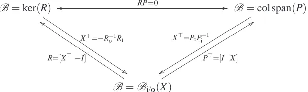
Consider the input/output Bi/o(X), kernel ker(R), and image col span(P) representations ofB∈Ln and define
the partitionings
R=:Ri Ro
, Ro∈Rd×d and P=:
Pi
Po
, Pi∈Rn×n.
B=ker(R) oo RP=0 //
X⊤=−R−1o Ri
$ $ I I I I I I I I I I I I I I I I I I I I I
B=col span(P)
X⊤=PoPi−1
y y ssss ssss ssss ssss ssss ss
B=Bi/o(X)
R=[X⊤−I]
d d II II II II II II II II II III
P⊤=[I X]
[image:10.595.147.453.70.162.2]9 9 s s s s s s s s s s s s s s s s s s s s s s
Figure 2: Links among kernel, image, and input/output representations ofB∈Ln.
3.2 Solution of the total least squares problem
Approximation of the data matrix C with a model B in the model class Ln is equivalent to finding a matrixCb∈
Rm×(n+d)with rank at most n. In the case when the approximation criterion iskC−CbkF(total least squares problem)
orkC−Cbk2, the problem has a solution in terms of the singular value decomposition of C. The result is known as the Eckart–Young–Mirsky low-rank matrix approximation theorem [17]. We state it in the next lemma.
Lemma 4 (Matrix approximation lemma). Let C=UΣV⊤be the singular value decomposition of C∈Rm×(n+d)and partition the matrices U ,Σ=: diag(σ1, . . . ,σn+d), and V as follows:
U=:
n d
U1 U2
m , Σ=:
n d
Σ
1 0
0 Σ2 n
d and V=:
n d
V1 V2
n+d . (SVD PRT)
Then the rank-n matrixCb∗=U1Σ1V1⊤is such that kC−Cb∗kF= min
rank(C)b≤nk
C−CbkF= q
σ2
n+1+···+σn+d2 . The solutionCb∗is unique if and only ifσn+16=σn.
The solution of the total least squares problem (TLS) trivially follows from Lemma 4.
Theorem 5 (Solution of the total least squares problem). Let C=UΣV⊤be the singular value decomposition of C and partition the matrices U ,Σ, and V as in (SVD PRT). Then a total least squares approximation of C inLnis
b
Ctls=U1Σ1V1⊤, Bbtls=ker(V2⊤) =col span(V1), and the total least squares misfit is
Mtls(C,B) =kΣ2kF= q
σ2
n+1+···+σn+d2 , where Σ2=: diag(σn+1, . . . ,σn+d). A total least squares approximation always exists. It is unique if and only ifσn6=σn+1.
Note 6 (Non-generic total least squares problems). The optimal approximating modelBbtlsmight have no input/output
representation (I/O repr). In this case, the optimization problem (TLS1) has no solution. By suitable permutation of the variables, however, (TLS1) can be made solvable, so thatXbtlsexists andBbtls=Bi/o(Xbtls).
The issue of whether the total least squares problem is generic or not is not related to the approximation of the data per se but to the possibility of representing the optimal modelBbtlsin the form (I/O repr), i.e.,
to the possibility of imposing a given input/output partition onBbtls.
3.3 Generalized total least squares problem
Let Wℓ∈Rm×mand Wr∈R(n+d)×(n+d)be given positive definite matrices and define the following generalized total least squares misfit function
Mgtls(C,B) =min
b
C∈B
√Wℓ(C−Cb)√Wr
F. (Mgtls)
Problem 7 (Generalized total least squares). Given a data matrix C∈Rm×(n+d), positive definite weight matrices Wℓ
and Wr, and a complexity specification n, solve the optimization problem
{Bbgtls,Cbgtls}=arg min
b B∈Ln
Mgtls(C,B). (GTLS)
The solution of the generalized total least squares problem can be obtained from the solution of a total least squares problem for a modified data matrix.
Theorem 8 (Solution of the generalized total least squares problem). Define the modified data matrix
Cm:= √
WℓC√Wr,
and letCbm,tls,Bbm,tls=ker(Rm,tls) =col span(Pm,tls)be a total least squares approximation of CminLn. Then a solution of the generalized total least squares problem (GTLS) is
b
Cgtls= √Wℓ−1Cbm,tls √Wr−1, b
Bgtls=ker Rm,tls√Wr=col span √Wr−1Pm,tls
and the corresponding generalized total least squares misfit is Mgtls(C,Bgtls) =Mtls(Cm,Bm,tls). A generalized total
least squares solution always exists. It is unique if and only ifBbm,tlsis unique.
Robust algorithms for solving the generalized total least squares problem without explicitly computing the inverses (√Wℓ)−1and(√Wr)−1are proposed in [86, 85, 88]. These algorithms give better accuracy when the weight matrices
are nearly rank deficient. In addition, they can treat the singular case, which implies that some rows and/or columns of C are considered exact and are not modified in the solutionC.b
If the matrices Wℓand Wrare diagonal, i.e., Wℓ=diag(wℓ,1, . . . ,wℓ,m), where wℓ∈Rm+and Wr=diag(wr,1, . . . ,wr,n+d),
where wℓ∈Rn+d+ the generalized total least squares problem is called scaled total least squares.
4
Weighted total least squares
For a given positive definite weight matrix W ∈Rm(n+d)×m(n+d)define the weighted matrix norm
kCkW := q
vec⊤(C⊤)W vec(C⊤) and the weighted total least squares misfit function
Mwtls(C,B):=min
b
C∈Bk
C−CbkW. (Mwtls)
The approximation problem with weighted total least squares misfit function is called the weighted total least squares problem.
Problem 9 (Weighted total least squares). Given a data matrix C∈Rm×(n+d), a positive definite weight matrix W , and a complexity specification n, solve the optimization problem
{Bbwtls,Cbwtls}:=arg min
B∈LnMwtls(C,
B). (WTLS)
The motivation for considering the weighted total least squares problem is that it defines the maximum likeli-hood estimator for the errors-in-variables model when the measurement noise ˜C=A˜ B˜ is zero mean, normally distributed, with a covariance matrix
Note 10 (Element-wise weighted total least squares). The special case when the weight matrix W is diagonal is called element-wise weighted total least squares (element-wise weighted total least squares). It corresponds to an errors-in-variables problem with uncorrelated measurement errors. Let W =diag(w1, . . . ,wm(n+d))and define the m×(n+d) weight matrixΣbyΣi j:=w(i−1)(n+d)+j. Denote by⊙the element-wise product A⊙B=
ai jbi j
. Then
k∆CkW =kΣ⊙∆CkF.
Note 11 (Total least squares as an unweighted weighted total least squares). The extreme special case when W =I is called unweighted. Then the weighted total least squares problem reduces to the total least squares problem. The total least squares misfit Mtls weights equally all elements of the correction matrix∆C. It is a natural choice when there is no prior knowledge about the data. In addition, the unweighted case is computationally easier to solve than the general weighted case.
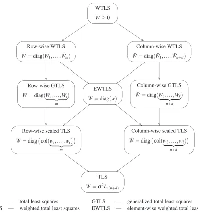
Special structure of the weight matrix W results in special weighted total least squares problems. Figure 3 shows a hierarchical classification of various problems considered in the literature. From top to bottom the generality of the problems decreases: on the top is a weighted total least squares problem for a general positive semi-definite weight matrix and on the bottom is the classical total least squares problem. In between are weighted total least squares problems with (using the stochastic terminology) uncorrelated errors among the rows, among the columns, and among all elements (element-wise weighted total least squares case). Row-wise and column-wise uncorrelated weighted total least squares problems, in which the row or column weight matrices are equal are generalized total least squares problems with respectively Wℓ=I and Wr=I. In order to express easily the structure of the weight matrix in the case of column-wise uncorrelated errors, we introduce the weight matrix ¯W as follows: cov vec(C˜)=σ2W¯−1, compare with (∗∗), where ˜C is transposed.
With W=I, (WTLS) coincides with the total least squares problem (TLS). Except for the special case of general-ized total least squares, however, the weighted total least squares problem has no closed form solution in terms of the singular value decomposition. As an optimization problem it is non-convex, so that the currently available solution methods do not guarantee convergence to a global optimum solution. In the rest of this section, we give an overview of solution methods for the weighted total least squares problem, with emphasis on the row-wise weighted total least squares case, i.e., when the weight matrix W is block diagonal W=diag(W1, . . . ,Wm), Wi∈R(n+d)×(n+d), Wi>0. In the errors-in-variables setting, this assumption implies that the measurement errors ˜ci and ˜cj are uncorrelated for all
i,j=1, . . . ,m, i6= j, which is a reasonable assumption for most applications.
Similarly to the total least squares and generalized total least squares problems, the weighted total least squares problem is a double minimization problem. The inner minimization is the search for the best approximation of the data in a given model and an outer minimization is the search for the model. First, we solve the inner minimization problem—the misfit computation.
4.1 Best approximation of the data by a given model
Since the model is linear, (Mwtls) is a convex optimization problem with an analytic solution. In order to give explicit formulas for the optimal approximationCbwtlsand misfit Mwtls(C,B), however, we need to choose a particular parameterization of the given modelB. We state the results for the kernel and the image representations. The results
for the input/output representation follow from the given ones by the substitutions R7→X⊤ −Iand P7→ I X⊤
.
Theorem 12 (Weighted total least squares misfit computation, kernel representation version). Let ker(R)be a minimal kernel representation ofB∈Ln. The best weighted total least squares approximation of C in B, i.e., the solution
of (Mwtls), is
b
cwtls,i= I−Wi−1R⊤(RWi−1R⊤)−1R
ci, for i=1, . . . ,m with the corresponding misfit
Mwtls C,ker(R)
= s
m
∑
i=1c⊤i R⊤(RW−1
WTLS
W≥0
z z uuuu uuuu uuuu u $ $ I I I I I I I I I I I I I Row-wise WTLS
W=diag(W1, . . . ,Wm)
# # G G G G G G G G G G G G G G G Column-wise WTLS ¯
W=diag(W¯1, . . . ,W¯n+d)
{ { wwww wwww wwww www Row-wise GTLS
W=diag(Wr, . . . ,Wr | {z }
m )
EWTLS
W=diag(w)
| | yyyy yyyy yyyy yy " " E E E E E E E E E E E E E E Column-wise GTLS ¯
W =diag(Wℓ, . . . ,Wℓ
| {z } n+d
)
Row-wise scaled TLS
W=diag col(wr, . . . ,wr) | {z }
m # # G G G G G G G G G G G G G
Column-wise scaled TLS
¯
W =diag col(wℓ, . . . ,wℓ
| {z } n+d ) { { wwww wwww wwww TLS
W=σ2I m(n+d) WV UT PQ RS WV UT PQ RS WV UT PQ RS WV UT PQ RS WV UT PQ RS WV UT PQ RS WV UT PQ RS WV UT PQ RS WV UT PQ RS
TLS — total least squares GTLS — generalized total least squares
[image:13.595.94.489.73.494.2]WTLS — weighted total least squares EWTLS — element-wise weighted total least squares
Figure 3: Hierarchy of weighted total least squares problems according to the structure of the weight matrix W . On the left side are weighted total least squares problems with row-wise uncorrelated measurement errors and on the right side are weighted total least squares problems with column-wise uncorrelated measurement errors.
Theorem 13 (Weighted total least squares misfit computation, image representation version). Let col span(P) be a minimal image representation ofB∈Ln. The best weighted total least squares approximation of C inBis
b
cwtls,i=P(P⊤WiP)−1P⊤Wici, for i=1, . . . ,m with the corresponding misfit
Mwtls C,col span(P) = s m
∑
i=1c⊤i Wi I−P(P⊤WiP)−1P⊤Wi
ci. (MwtlsP)
4.2 Optimization over the model parameters
The remaining problem—the minimization with respect to the model parameters is a nonconvex optimization problem that in general has no closed form solution. For this reason numerical optimization methods are employed for its solution.
problem but includes the weighted total least squares problem with diagonal weight matrix and d=1 as a special case. The restriction to more general weighted total least squares problems comes from the fact that the Riemannian singular value decomposition framework is derived for matrix approximation problems with rank reduction by one. De Moor proposed an algorithm resembling the inverse power iteration algorithm for computing the solution. The method, however, has no proven convergence properties.
The maximum likelihood principle component analysis method of Wentzell et al. [90] is an alternating least squares algorithm. It applies to the general weighted total least squares problems and is globally convergent, with linear convergence rate. The method of Premoli and Rastello [64] is a heuristic for solving the first order optimality condition of (WTLS). A solution of a nonlinear equation is sought instead of a minimum point of the original opti-mization problem. The method is locally convergent with super linear convergence rate. The region of convergence around a minimum point could be rather small in practice. The weighted low rank approximation framework of Man-ton et al. [44] proposes specialized optimization methods on a Grassman manifold. The least squares nature of the problem is not exploited by the algorithms proposed in [44].
The Riemannian singular value decomposition, maximum likelihood principle component analysis, Premoli–Rastello, and weighted low rank approximation methods differ in the parameterization of the model and the optimization algorithm used, see Table 1.
Method Representation Algorithm
Riemannian singular value decomposition kernel inverse power iteration maximum likelihood principle component analysis image alternating projections
[image:14.595.54.547.318.399.2]Premoli–Rastello input/output iteration based on heuristic linearization weighted low rank approximation kernel Newton method
Table 1: Model representations and optimization algorithms used in the methods of [12, 90, 64, 44, 72].
5
Structured total least squares
The total least squares problem is a tool for approximate modeling by a static linear model. Similarly, the structured total least squares problem with block-Hankel structured data matrix is a tool for approximate modeling by a linear time-invariant dynamic model. In order to show how the block-Hankel structure occurs, consider a difference equation represented of the an linear time-invariant model
R0wt+R1wt+1+···+Rlwt+l =0. (KER) Here R0, . . . ,Rlare the model parameters and the integer l is the lag of the equation. For t=1, . . . ,T−l, the difference equation (KER) is equivalent to the block-Hankel structured system of equations
R0 R1 ··· Rl
w1 w2 ··· wT−l
w2 w3 ··· wT−l+1
..
. ... ...
wl+1 wl+2 ··· wT
| {z }
Hl(w)
=0. (Hank eqn)
Thus the constraint that a time series w= w(1), . . . ,w(T)is a trajectory of the linear time-invariant model implies rank deficiency of the block-Hankel matrixHl(w).
5.1 Examples
Deconvolution
The convolution of the (scalar) sequences
(. . . ,a−1,a0,a1, . . .) and (. . . ,x−1,x0,x1, . . .) is the sequence(. . . ,b−1,b0,b1, . . .)defined as follows:
bi= ∞
∑
j=−∞xjai−j. (CONV)
Assume that xj =0 for all j<1 and for all j>n. Then (CONV) for i=1, . . . ,m can be written as the following structured system of equations
a0 a−1 ··· a1−n
a1 a0 ··· a2−n
..
. ... ...
am−1 am+n−2 ··· am−n
| {z }
A x1 x2 .. . xn
| {z } x = b1 b2 .. . bm
| {z } b
. (CONV’)
Note that the matrix A is Toeplitz structured and is parameterized by the vector a=col(a1−n, . . . ,am−1)∈Rm+n−1.
The aim of the deconvolution problem is to find x, given a and b. With exact data the problem boils down to solving the system of equations (CONV’). By construction it has an exact solution. Moreover the solution is unique whenever A is of full column rank, which can be translated to a persistency of excitation condition on a, see [92].
The deconvolution problem is more realistic and more challenging when the data a,b is perturbed. We assume that m>n, so that the system of equations (CONV’) is overdetermined. Because both a and b are perturbed and the A matrix is structured, the deconvolution problem is a total least squares problem with structured data matrix C=A b, A Toeplitz and b unstructured.
Linear prediction
In many signal processing applications the sum of damped exponentials model
b yt =
l
∑
i=1cieditei(ωit+φi), where i := √
−1 (SDE)
is considered. Given an observed sequence (yd,1, . . . ,yd,T) (“d” stands for data), the aim is to find parameters {ci,di,ωi,φi}li=1 of a sum of damped exponentials model, such that the signal y given by (SDE) is close to theb observed one, e.g.,
min
yd,1
.. .
yd,T − b y1 .. . b yT .
Note that the sum of damped exponentials model is just an autonomous linear time-invariant model, i.e.,by is a free response of an linear time-invariant system. Thereforeby satisfies a homogeneous linear difference equation
b yt+
l
∑
τ=1
aτbyt+τ =0. (LP)
For a time horizon t=1, . . . ,T , with T >l+1, (LP) can be written as the structured system of equations b
y1 by2 ··· ybl b
y2 by3 ··· byl+1
..
. ... ...
b
ym bym+1 ··· byT−1 a1 a2 .. . al =− b yl+1 b yl+2 .. . b yT ,
where m :=T−l. Therefore, the Hankel matrix Hl+1(by) with l+1 columns, constructed from by is rank deficient.
Conversely, ifHl+1(yb)has a one dimensional left kernel, then by satisfies the linear recursion (LP). Therefore, the
linear prediction problem is the problem of finding the smallest in some sense (e.g., 2-norm) correction∆y on the given sequence ydthat makes a block-Hankel matrixHl+1(by)constructed from the corrected sequence by :=yd−∆y rank deficient. This is an structured total least squares problem Ax≈b with Hankel structured data matrix C=A b.
Errors-in-variables identification
Consider the linear time-invariant system described by the difference equation
b yt+
l
∑
τ=1
aτbyt+τ = l
∑
τ=0
bτubt+τ (DE)
and define the parameter vector
x :=col(b0, . . . ,bl,−a0, . . . ,−al−1)∈R2l+1.
Given a set of input/output data(ud,1,yd,1), . . . ,(ud,T,yd,T)and an order specification l, we want to find the parameter x of a system that fits the data.
For a time horizon t=1, . . . ,T , (DE) can be written as the structured system of equations b
u1 ub2 ··· ubl+1 yb1 yb2 ··· ybl b
u2 ub3 ··· ubl+2 yb2 yb3 ··· byl+1
..
. ... ... ... ... ...
b
um ubm+1 ··· ubT ybm bym+1 ··· byT−1 x=
b yl+1 b yl+2 .. . b yT
, (DE’)
where m :=T−l. We assume that the time horizon is large enough to ensure m>2l+1. The system (DE’) is satisfied for exact data and a solution is the true value of the parameter x. Moreover, under additional assumption on the input (persistency of excitation) the solution is unique.
For perturbed data an approximate solution is sought and the fact that the system of equation (DE’) is structured suggests the use of the structured total least squares method. Under appropriate conditions for the data generating mechanism an structured total least squares solution provides a maximum likelihood estimator. The structure arising in the errors-in-variables identification problem is C=H⊤
l (ud) Hl⊤(yd)
.
5.2 History of the structured total least squares problem
The origin of the structured total least squares problem dates back to the work of Aoki and Yue [4], although the name “structured total least squares” appeared only 23 years later in the literature [12]. Aoki and Yue consider a single input single output system identification problem, where both the input and the output are noisy (errors-in-variables setting) and derive a maximum likelihood solution. Under the normality assumption for the measurement errors, a maximum likelihood estimate turns out to be a solution of the structured total least squares problem. Aoki and Yue approach the optimization problem in a similar way to the one presented in Section 5.3: they use classical nonlinear least squares minimization methods for solving an equivalent unconstrained problem.
because of their simplicity. For example, the method of Cadzow is an iterative method that alternates between un-structured low rank approximation and structure enforcement, thereby only requiring singular value decomposition computations and manipulation of the matrix entries.
Tufts and Shah propose in [80], a noniterative method for Hankel structured total least squares approximation that is based on perturbation analysis and provides nearly optimal solution for high signal-to-noise ratio (SNR). In a statistical setting, this method achieves the Cramer-Rao lower bound asymptotically as the SNR tends to infinity. Noniterative methods for solving the linear prediction problem (which, as shown in Section 5.1, is equivalent to Hankel structured total least-squares problem) are proposed by Tufts and Kumaresan in their seminal work [79, 33].
Abatzoglou et al. [1] are considered to be the first who formulated a structured total least squares problem. They called their approach constrained total least squares and motivate the problem as an extension of the total least squares method to matrices with structure. The solution approach adopted by Abatzoglou et al. is closely related to the one of Aoki and Yue. Again an equivalent optimization problem is derived, but it is solved numerically using a Newton-type optimization method.
Shortly after the publication of the work on the constrained total least squares problem, De Moor [12] lists many applications of the structured total least squares problem and outlines a new framework for deriving analytical prop-erties and numerical methods. His approach is based on the Lagrange multipliers and the basic result is an equivalent problem, called Riemannian singular value decomposition, which can be considered as a “nonlinear” extension of the classical singular value decomposition. As an outcome of the new problem formulation, an iterative solution method based on the inverse power iteration is proposed.
Another algorithm for solving the structured total least squares problem (even withℓ1 and ℓ∞norm in the cost function), called structured total least norm, is proposed by Rosen et al. [67]. In contrast to the approaches of Aoki, Yue and Abatzoglou et al., Rosen et al. solve the problem in its original formulation. The constraint is linearized around the current iteration point, which results in a linearly constrained least squares problem. In the algorithm of Rosen et al., the constraint is incorporated in the cost function by adding a multiple of its residual norm.
The weighted low rank approximation framework of Manton et al. [44] has been extended in [70, 71] to structured low rank approximation problems. All problem formulations and solution methods cited above, except for the ones in the structured low rank approximation framework, aim at rank reduction of the data matrix C by one. A generalization of the algorithm of Rosen et al. to problems with rank reduction by more than one is proposed by Van Huffel et al. [83]. It involves, however, Kronecker products that unnecessary inflate the dimension of the involved matrices.
When dealing with a general affine structure the constrained total least squares, Riemannian singular value decom-position, and structured total least norm methods have cubic computational complexity per iteration in the number of measurements. Fast algorithms with linear computational complexity are proposed by Mastronardi et al. [38, 55, 53] for special structured total least squares problems with data matrix C=A bthat is Hankel or composed of a Hankel block A and an unstructured column b. They use the structured total least norm approach but recognize that a matrix appearing in the kernel subproblem of the algorithm has low displacement rank. This structure is exploited using the Schur algorithm.
The structured total least squares solution methods outlined above point out the following issues:
• structure: the structure specification for the data matrix C varies from general affine to specific affine, like Hankel/Toeplitz, or Hankel/Toeplitz block augmented with an unstructured column,
• rank reduction: all methods, except for [83, 70, 71], reduce the rank of the data matrix by one,
• computational efficiency: the efficiency varies from cubic for the methods that use a general affine structure to linear for the efficient methods of Lemmerling et al. [38] and Mastronardi et al. [55] that use a Hankel/Toeplitz type structure.
Efficient algorithms for problems with block-Hankel/Toeplitz structure and rank reduction with more than one are proposed by Markovsky et al. [50, 49, 48]. In addition, a numerically reliable and robust software implementation is available [46].
5.3 Structured total least squares problem formulation and solution method
LetS :Rnp→Rm×(n+d)be an injective function. A matrix C∈Rm×(n+d)is said to beS-structured if C∈image(S).
the parameter space of the structureS.
The aim of the structured total least squares problem is to perturb as little as possible a given parameter vector p by a vector∆p, so that the perturbed structured matrixS(p+∆p)becomes rank deficient with
rank at most n.
Problem 14 (Structured total least squares). Given a data vector p∈Rnp, a structure specificationS :Rnp→Rm×(n+d),
and a rank specification n, solve the optimization problem
∆pstls=arg min
∆p k∆pk subject to rank
S(p−∆p)≤n.
In what follows, we will use the input/output representation
S(p−∆p)Xext=0, Xext:=
X −I
of the rank constraint, so that the structured total least squares problem becomes the following parameter optimization problem
b
Xstls=arg min
X,∆pk∆pk subject to
S(p−∆p)
X −I
=0. (STLSX) The structured total least squares problem is said to be affine structured if the functionS is affine, i.e.,
S(p) =S0+
np
∑
i=1Sipi, for all p∈Rnp and for some Si,i=1, . . . ,np. (AFF)
In an affine structured total least squares problem, the constraintS(p−∆p)Xext=0 is bilinear in the decision variables
X and∆p.
Lemma 15. LetS :Rnp →Rm×(n+d)be an affine function. Then
S(p−∆p)Xext=0 ⇐⇒ G(X)∆p=r(X),
where
G(X):=vec (S1Xext)⊤
··· vec (SnpXext)⊤
∈Rmd×np, (G)
and
r(X):=vec S(p)Xext⊤∈Rmd.
Using Lemma 15, we rewrite the affine structured total least squares problem as follows
min X
min
∆p k∆pk subject to G(X)∆p=r(X)
. (STLS′X)
The inner minimization problem has an analytic solution, which allows to derive an equivalent optimization problem.
Theorem 16 (Equivalent optimization problem for affine structured total least squares). Assuming that np≥md, the affine structured total least squares problem (STLS′X) is equivalent to
min X r
⊤(X)Γ†(X)r(X) where Γ(X):=G(X)G⊤(X), (STLS′′
X)
andΓ†is the pseudoinverse ofΓ.
The significance of Theorem 16 is that the constraint and the decision variable∆p in problem (STLS′X) are elimi-nated. Typically the number of elements nd in X is much smaller than the number of elements npin the correction∆p. Thus the reduction in the complexity is significant.
![Table 1: Model representations and optimization algorithms used in the methods of [12, 90, 64, 44, 72].](https://thumb-us.123doks.com/thumbv2/123dok_us/8495010.345659/14.595.54.547.318.399/table-model-representations-optimization-algorithms-used-methods.webp)
