Effects of the Number of Hidden Nodes Used in a
Structured-based Neural Network on the Reliability of
Image Classification
Weibao Zou1,2, Yan Li3 and Arthur Tang4 1
Department of Electronic and Information Engineering, The Hong Kong Polytechnic University, Hong Kong
2Shenzhen Institute of Advanced Technology, China
3
Department of Mathematics and Computing, The University of Southern Queensland, Australia
4
University of Central Florida, USA
Abstract
A structured-based neural network (NN) with Backpropagation Through Structure (BPTS)
algorithm is conducted for image classification in organizing a large image database, which is a
challenging problem under investigation. Many factors can affect the results of image
classification. One of the most important factors is the architecture of a NN which consists of
input layer, hidden layer and output layer. In this study, only the numbers of nodes in hidden
layer (hidden nodes) of a NN are considered. Other factors are kept unchanged. Two groups of
experiments including 2940 images in each group are used for the analysis. The assessment of the
effects for the first group is carried out with features described by image intensities, and, the
second group uses features described by wavelet coefficients. Experimental results demonstrate
that the effects of the numbers of hidden nodes on the reliability of classification are significant
and non-linear. When the number of hidden nodes is 17, the classification rate on training set is
choice for the number of hidden nodes for the image classification when a structured-based NN
with BPTS algorithm is applied.
Keywords: hidden nodes, Backpropagation Through Structure, image classification, neural network, features set
I. INTRODUCTION
MAGE content representation is a challenging problem in organizing a large image
database. Most of the applications represent images using low level visual features, such as color, texture, shape and spatial layout in a very high dimensional feature space, either globally or locally. However, the most popular distance metrics, such as Euclidean distance, cannot guarantee that the contents are similar even though their visual features are very close in the high dimensional space. With a structured-based neural network, the image classification using features described by Independent Component Analysis (ICA) coefficients and wavelet coefficients proposed by Zou et al [1] [2] is an effective solution to this problem. An image is represented by a tree structure of features. Both features and the spatial relationships among them are considered since they play more important roles in characterizing image contents and convey more semantic meanings.
I
classification.
The reliability of image classification is also affected by many other factors, such as input features of a neural network, methods of encoding nodes, tree structural representation of images and the amount of samples for training the neural network. In this study we only investigate effects of the number of hidden nodes. All other factors are kept unchanged.
The number of hidden nodes is determined by different methods in literature. The optimal number of hidden nodes is derived by log(T), where T is the number of training samples [7]. The number of input training pattens is used to calculate the number of hidden nodes [8]. Nocera and Quelavoine proposed a method which is able to reduce the hidden nodes but still makes the neural network work properly [9]. A series of different hidden nodes were tested to classify sonar targets in [10].
The number of hidden nodes is defined as the width of a neural network [11]. The hidden layer of the neural network must be wide enough so that the result of a classification can be accurate, but too wide would result in over-fitting [12]. Therefore, the critical issue is “what is the most appropriate number of hidden nodes for a structured-based neural network for image classification?”. This study aims to conduct a systematic investigation into the effects of the numbers of hidden nodes used in a structured-based neural network on the reliability of image classification.
This introduction is followed by a brief of the structured-based NN and the definition of the reliability of image classification. The feature sets and image database are then described in Sections III and IV. Two groups of experiments are carried out and the results are discussed and analysed in Section V. The analysis of the results prompts more experiments, which further support the conclusions drawn in Section VI.
II. STRUCTURED-BASED NEURAL NETWORK FOR IMAGE CLASSIFICATION
A. Image classification with a structured-based neural network
characterized by relatively poor representations in data structures, such as static patterns or sequences. Most structured information presented in the real world, however, can hardly be represented by simple sequences. Although many early approaches based on syntactic pattern recognition were developed to learn structured information, devising a proper syntax is often a very difficult task because domain knowledge is often incomplete or insufficient. On the contrary, graph representations vary with the sizes of input units and can organize data flexibly. Recently, neural networks for processing data structures have been proposed by Sperduti [13]. It has been shown that they can be used to process data structures using an algorithm, namely back-propagation through structure (BPTS). The algorithm extends the unfolding time carried out by back-propagation through time (BPTT) in the case of sequences. A general framework of adaptive processing of data structures is introduced by Tsoi [14] and Frasconi et al [3][14-15]. In the BPTS algorithm, a copy of the same neural network is used to encode every node in a graph. Such an encoding scheme is flexible enough to allow the method to deal with directed acyclic graphs of different internal structures with different number of nodes. Moreover, the model can also naturally integrate structural information into its processing. An improved BPTS algorithm by Cho et al is used in this study. For details, see [6] and [16].
B. Reliability in image classification
Reliability is a widely used concept in engineering and industry. A generally acceptable definition given by the British Standards Institution is as follows [17]:
“Reliability is the characteristic of an item expressed by the probability that it will perform a required function under stated conditions for a stated period of time.”
In the case of image classification, it is assumed that the accuracy rate of the image classification is a good measure for the reliability. This implies that the larger the rate, the better or more reliable the performance.
III. DESCRIPTION OF FEATURE SETS FOR NEURAL NETWORK
It is now pertinent to provide the description of features as attributes for the neural network and explain the methodology used in this paper.
Several factors affect the reliability of image classification. However, as explained previously, only the numbers of hidden nodes are investigated in this study. Other factors are kept unchanged.
There are two groups of experiments carried out in this section. Different features are divided into two groups: features described by wavelet coefficients used in the first group and those described by image intensities in the second group. For each group, a set of different numbers of hidden nodes are selected to analyze the relationship between the hidden nodes and the reliability of image classification. As the features are used to form the two groups, it is necessary to describe the features as below.
A. Features extracted by wavelets transformation
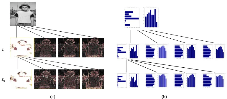
With the goal of extracting features, as an application of the wavelet decomposition performed by a computer, a discrete wavelet transformation is considered. A tree representation of an image decomposed by wavelets transformation is shown in Fig. 1(a). At level one ( 1), the original image (the top image) is decomposed into four bands. The
leftmost one in the line of 1 is the low-pass band, and the three ones on the right hand
side are the high-pass bands. At level two (L2), the previous low-pass band is decomposed
into four bands. The leftmost one in the line of 2 is the low-pass band, and the other
three are the high-pass bands, which represent the characteristics of the image in the horizon, vertical, and diagonal views, respectively. From Fig. 1(a), it can be found that
L
L
the basic energy and the edges of an object can be observed in low-pass band and high-pass bands at each level.
1
L
2
L
(a) (b)
Fig. 1. A tree structural representation of an image: (a) An image decomposed by wavelets transformation at two levels; (b) A tree representation of histograms of projections of wavelet coefficients corresponding to the images in (a)
The features of an object can be described by the distribution of wavelet coefficients. It is found that wavelet coefficients corresponding to the edges of the object are greater than a certain threshold value. The wavelet coefficients which are greater than the threshold are selected into a feature set. These coefficients are projected onto the x-axis and y-axis directions, respectively. The edges of the object, therefore, can be described by the distribution of the projections of wavelet coefficients, which are statistics by histograms with 8 bins in the x direction and 8 bins in the y direction.
[image:6.612.122.507.118.287.2]values are smaller than 127. Therefore, the number of pixels contained in the first bar is zero. The length of the bar is also zero. In the second region, from rows 68 to 134, there are 3500 pixels whose gray values are smaller than 127. So the length of second bar is 3500. The features for the remaining regions can be deduced in a similar way. The left top figure of Fig. 1(b) is drawn as an example. The processing procedures are the same for the histograms of projections in x-axis.
The tree representation of an image described by histograms of projections of wavelet coefficients is illustrated in Fig. 1(b).
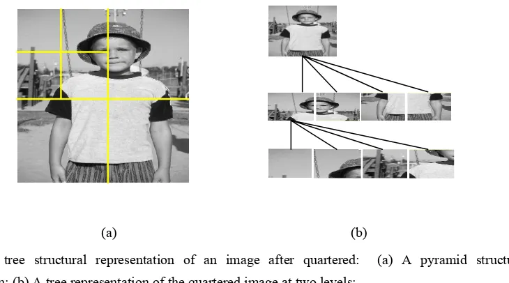
[image:7.612.143.508.268.471.2](a) (b)
Fig. 2. A tree structural representation of an image after quartered: (a) A pyramid structural representation; (b) A tree representation of the quartered image at two levels;
B. Features extracted by image quartered
Conventionally, the features for image classification are visual features, such as color, texture and shape. The intensities are used as conventional features in this study. Similar to last section, in the tree structural representation, the contents of a region are characterized by the histograms of the intensities projected onto x and y directions, respectively. The histograms are statistics with 8 bins in each direction. Totally, 16 features are taken as input attributes for the neural network.
the top left region) is quartered again into four regions at the second level. This idea is based on that if the region contains an object, the object will be very different from the background. This results in a large entropy.
IV. IMAGE SETS FOR THE EXPERIMENT
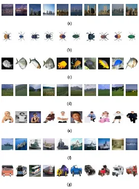
Seven categories of images, namely, building, beetle, fish, grass, people, warship and vehicle, are adopted in this study. In each category of images, there are ten independent images as shown in Fig. 3.
(a)
(b)
(c)
(d)
(e)
(f)
(g)
Fig. 3. Images for experiments: (a) Building; (b) Beetle; (c) Fish; (d) Grass; (e) People; (f) Warship; (g) Vehicle
[image:8.612.165.447.240.624.2]original image, and it shifts from left to right, then top to bottom. Of course, the object must be contained in the window. However, the background is changing with the shifting window. Corresponding to each window shift, a new image is generated. Therefore, from each image, 60 new images are generated from this translational operation.
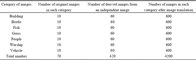
For each category of images, there are 600 derived images except the original one. Totally, 4200 images are derived from these original images. The information of the image set is tabulated in Table I. There are three kinds of data sets in the project. One is training set, another test set and the rest validation set. Together with the original images, 1470 images are used for training the neural network and other 1470 images are used for testing. The rest 1470 images are included in the validation set which is used to validate if the overfitting occurs.
TABLE I IMAGE DATABASES FOR THE STUDY
Category of images Number of original images in each category
Number of derived images from an independent image
Number of images in each category after image translation
Building 10 60 600
Beetle 10 60 600
Fish 10 60 600
Grass 10 60 600
People 10 60 600
Warship 10 60 600
Vehicle 10 60 600
Total number 70 420 4200
V. EFFECTS OF THE NUMBERS OF HIDDEN NODES ON THE RELIABILITY OF IMAGE
CLASSIFICATION
A. Selection of hidden nodes
With the two experimental groups, the number of hidden nodes varies from 10, 11, …
[image:9.612.103.512.353.479.2]TABLE II INFORMATION FOR THE NUMBER OF HIDDEN NODES
Category of images 7
Group 1 Histograms of the projections of image intensities Features used
as attributes Group2 Histograms of the projections of wavelet coefficients
Number of attributes 16
Depth of trees 3
Total number of nodes in tree 9
Number of epochs 5000
Number of hidden nodes 10 11 13 15 17 18 19 20 21 23 28 33 38 43
B. Experimental results and analysis
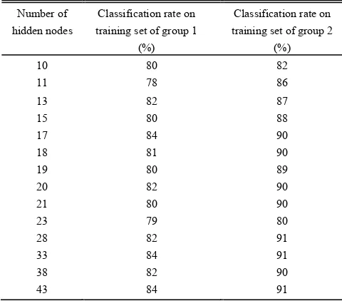
This section reports the classification performance. In this investigation, a single hidden-layer is sufficient for the neural classifier, which has 16 input nodes and 7 output nodes. The classification rates on training set and testing set are shown in Tables III and IV. A graphical presentation of Tables III and IV is also shown in Fig. 4(a) and (b), respectively.
TABLE III CLASSIFICATION RESULTS WITH DIFFERENT HIDDEN NODES ON TRAINING SET
Number of hidden nodes
Classification rate on training set of group 1
(%)
Classification rate on training set of group 2
(%)
10 80 82
11 78 86
13 82 87
15 80 88
17 84 90
18 81 90
19 80 89
20 82 90
21 80 90
23 79 80
28 82 91
33 84 91
38 82 90
[image:10.612.93.519.95.203.2]43 84 91
TABLE IV CLASSIFICATION RESULTS WITH DIFFERENT HIDDEN NODES ON TESTING SET
Number of hidden nodes
Classification rate on testing set of group 1
(%)
Classification rate on testing set of group 2
(%)
10 63 74
[image:10.612.185.425.391.602.2] [image:10.612.186.425.651.718.2]13 58 86
15 76 85
17 79 87
18 53 81
19 54 85
20 79 84
21 77 89
23 65 71
28 66 89
33 78 86
38 72 89
43 59 86
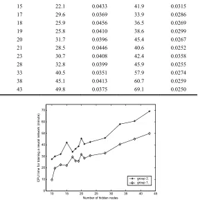
The time for training the neural network after 5000 epochs and mean-square error (MSE) are tabulated in Table V. MSE is used as a measure of the classification accuracy at root node during training the neural network. It is defined as follows:
n m y x y x MSE n i i i T i i ⋅ − −
=
∑
=1) ( ) (
(1)
where, is the target output at node i; is the output at node i. m is the number of
outputs of the neural network and n is the size of learning samples. The smaller the MSE,
i
x
y
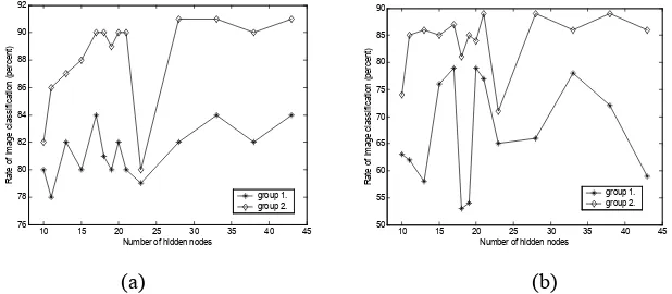
i [image:11.612.202.411.70.219.2]the better the performance. Graphical presentations of Table V are shown in Fig. 5 and Fig.6.
10 15 20 25 30 35 40 45 76 78 80 82 84 86 88 90 92
Number of hidden nodes
R at e of im age c las si fic at io n ( perc en t) group 1. group 2.
10 15 20 25 30 35 40 45 50 55 60 65 70 75 80 85 90
Number of hidden nodes
R at e of im age c las si fic at ion (pe rc ent ) group 1. group 2.
[image:11.612.150.459.446.581.2](a) (b)
Fig. 4 Variations of image on training set; (b) rate on
TABLE V CPU TIME AND MSE FOR TRAINING A NEURAL NETWORK classification rate with different hidden nodes: (a) rate testing set
Results of group 1 Results of group 2 Numb
CP E CP E
er of
hidden nodes U time MS
(min)
U time MS
(min)
10 9.6 0.0520 27.5 0.0351
11 19.6 0.0467 29.9 0.0342
[image:11.612.165.448.635.713.2]15 22.1 0.0433 41.9 0.0315
17 29.6 0.0369 33.9 0.0286
18 25.9 0.0456 36.5 0.0269
19 25.8 0.0410 38.6 0.0299
20 31.7 0.0396 45.4 0.0267
21 28.5 0.0446 40.6 0.0252
23 30.7 0.0408 42.4 0.0358
28 32.8 0.0399 45.9 0.0255
33 40.5 0.0351 57.9 0.0274
38 45.1 0.0413 60.7 0.0259
43 49.8 0.0375 69.1 0.0250
10 15 20 25 30 35 40 45 0
10 20 30 40 50 60 70
Number of hidden nodes
C
P
U
t
im
e f
or
t
rai
ni
ng
a ne
ur
al
n
et
w
or
k (m
in
ut
e)
group 2. group 1.
Fig. 5 Variations of CPU time with the different numbers of h dden nodes i
10 15 20 25 30 35 40 45
0.01 0.015 0.02 0.025 0.03 0.035 0.04 0.045 0.05 0.055
Number of hidden nodes
M
S
E
of
t
he out
put
group 2. group 1.
Fig. 6 Variations of MSE with the different numbers of hidden nodes
[image:12.612.164.450.70.359.2] [image:12.612.215.388.402.538.2]The best rate of 91% is also achieved when the numbers of hidden nodes are 28, 33 and 43, respectively. However, these hidden numbers are much larger than 17 and cause an increase in computational complexity and much more training time. It can be derived from Table V that the CPU times, from 33.9 minutes (for 17 hidden nodes) to 45.9 minutes (for 28 hidden nodes), 57.9 minutes (for 33 hidden nodes) and 69.1 minutes (for 43 hidden nodes), are increased by 35.4%, 70.8% and 103.8%, respectively. The MSEs, from 0.0286 to 0.0255, 0.0274 and 0.0250, are decreased by 10.8%, 4.2% and 12.6%, respectively. However, the image classification rate is just improved by 1%, from 90% to 91%. Therefore, the number 17 is a trade-off value for hidden nodes for getting a better classification rate without the increase of the computation complexity.
For the first experiment group, when the number of hidden nodes is 17, the classification rate is the best (84%). The same rate is also obtained for the hidden numbers of 33 and 43. However, the least CPU time is required when the hidden nodes are 17. This indicates that when the number of hidden nodes is 17, the classification rate is better or the best with a fast speed.
With the trained neural network, the testing is carried out with another set of images not used in the training set. From Table IV and Fig. 4(b), it is found that the classification rate for group 2 is up to 89%. With 17 hidden nodes, its classification rate is 87%, close to the best. For the result of group 1, the rate is up to 79%. For 17 hidden nodes, its classification rate is the best. Apparently, the effects of the number of hidden nodes on the reliability of image classification are non-linear. The experiment results are more reliable when the number of hidden nodes is 17.
C. Analysis of overfitting
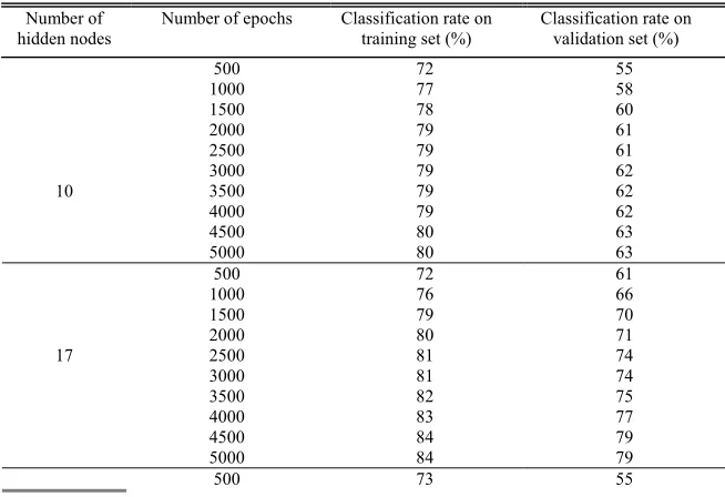
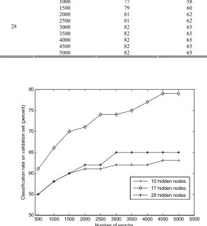
The overfitting is investigated by using the third data set, the validation data set. In the experiments, different numbers of epochs are tested from 1 to 5000 with a gap of 1. The classification rate validated by the validation data set with epochs at 500, 1000, 1500, 2000, 2500, 3000, 3500, 4000, 4500 and 5000 are presented in Table VI. The hidden nodes for the experiments are 10, 17 and 38, respectively. Its graphic representation of Table VI is also given in Fig. 7.
From Table VI and Fig.7, it is noticed that, for hidden nodes of 10, when training epoch is 500, its validated classification rate is 55% for group 1. With the increase of epochs, its classification rate increases. From epochs of 3000 to 4000, the rates remain the same at 62%. After that, the rate increases to 63%. From epochs of 4500 to 5000, the rates sit at 63% and do not change. Overall, the rate is becoming larger when the numbers of epoch is increasing. It eventually keeps almost the same value. It is validated that the overfitting dose not occur during training the neural network. For hidden nodes of 17 and 38, the same experimental results are obtained. They are similar for the results obtained by the hidden nodes of 11, 13, 15, 18, 19, 20, 21, 23, 33, 38 and 43. For the group 2, the similar results are obtained and it is concluded that the overfitting dose not occur in this study.
TABLE VI CLASSIFICATION RATE ON VALIDATION SET FOR GROUP 1
Number of hidden nodes
Number of epochs Classification rate on training set (%)
Classification rate on validation set (%)
500 72 55 1000 77 58 1500 78 60 2000 79 61 2500 79 61 3000 79 62 3500 79 62 4000 79 62 4500 80
10
5000 80
63 63 500 72 61 1000 76 66 1500 79 70 2000 80 71 2500 81 74 3000 81 74 3500 82 75 4000 83 77 4500 84
17
5000 84 79 79
[image:14.612.142.469.492.716.2]1000 77 58 1500 79 60 2000 81 62 2500 81 62 3000 82 65 3500 82 65 4000 82 65 4500 82
28
5000 82
65 65
500 1000 1500 2000 2500 3000 3500 4000 4500 5000 5500
50 55 60 65 70 75 80
Number of epochs
C
las
si
fic
at
ion
r
at
e
on v
al
idat
ion s
et
(
pe
rc
ent
)
10 hidden nodes. 17 hidden nodes. 28 hidden nodes
Fig. 7 Variations of classification rate on validation set with epochs of group 1
D. Statistical analysis of results
As observed from Tables III and IV, and Fig. 4, the classification rates vary with the number of hidden nodes. It is of great interest for researchers to examine whether or not the variations are of significance. Otherwise, any number of hidden nodes can be selected. In practice, however, it is unlikely as observable from Fig. 4. To test the significance, a t-test is carried out for the classification rates on both training and testing sets.
The test statistics take the following form [18]:
n s x t
/ μ
−
= (2)
where, is the number of samples; n
∑
= n n xi
[image:15.612.151.449.76.401.2]∑ =
− −
= n
i
i x
x n
s
1
2 ) ( 1
1 (4)
and μ is the smallest value among the samples.
Student’s t-test is separately carried out for the two groups. In this analysis, only the first group on the training set is taken as an example. In the group, the numbers of hidden nodes are 10, 11, 13, 17, 18, 19, 20, 21, 23, 28, 33, 38 and 43, respectively. The smallest rate on training set is 78% when the hidden nodes are 11. Therefore, one can make a hypothesis
0
H: μ=0.78
and the corresponding null hypothesis H0 is
a
H : not H0
Here, n=14 and resultant . These values are needed to be checked against the threshold in a standard table of
47 . 6
=
t
t values. In this example there are 13 degrees of freedom
(df) (= n-1); at 95% confidence level (α=0.05), (13) 2
α
t is 2.16 in the table of t values.
As the value obtained from this example is 6.47 which is greater than 2.16, 0 is
rejected in favour of and it is concluded that the variation of rate values is significant
at 95% confidence level.
t H
a
[image:16.612.204.409.539.609.2]H
TABLE VII. SIGNIFICANCE TEST ON CLASSIFICATION RATE*
t-Test results for rate values Classification rate Group 1 Group 2
Rate on training set Y (6.47) Y (8.98) Rate on testing set Y (5.61) Y (9.08) * Y = significant variation.
16 . 2 ) 13 (
2 =
α
t .
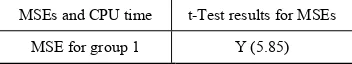
TABLE VIII. SIGNIFICANCE TEST ON MSES AND CPU TIME*
MSEs and CPU time t-Test results for MSEs
[image:16.612.218.394.678.710.2]MSE for group 2 Y (4.12) CPU time for group 1 Y (7.16) CPU time for group 2 Y (4.78) * Y = significant variation.
16 . 2 ) 13 (
2 =
α
t .
[image:17.612.219.395.73.125.2]Similar tests have also been carried out for the second group. The results are shown in Table VII. T-test has also been carried out for rate values on testing set and the results are included in Table VII. Meanwhile, the MSEs and CPU times on the training set are tested by t-test too. The results are provided in Table VIII. In these tables, ‘Y’ means a significant variation. It is noticed that, with different hidden nodes, the variations of classification rates, MSEs and CPU times are very significant for all the experimental results.
From the t-test results, it is observed that the effects of the number of hidden nodes on the image classification rate are significant. Therefore, the number of hidden nodes must be selected carefully.
VI. DISCUSSION
The experimental results in this paper demonstrate that the effects of the number of hidden nodes on the reliability of image classification are significant. Moreover, the rate of image classification is consistently better when the number of hidden nodes is 17. This means that the performance of image classification is reliable. However, there are a few issues to be cleared up before a reliable conclusion can be drawn.
From Table III and Fig. 4(a), it can be seen that when the number of hidden nodes of 21 is used, the rate of classification is 90% for the group 2; the same as the one when the hidden nodes are 17. However, its MSE values are smaller than the ones with the hidden nodes of 17 (by 11.9%). In addition, for the curve of group 2 in Fig. 4(b), it is noticed that when the number of hidden nodes is 21, the classification rate on the testing set is the highest. Therefore, the questions arising are:
consistently good?
(b) If yes, which should be recommended, ‘‘the number of 17’’ or ‘‘the number of 21’’? In order to obtain more reliable conclusions for this study, a group of experiments with different kind of features used as attributes are conducted for further investigation. In the experiments, the features sets are mixed, which consist of two parts: wavelet coefficients and ICA coefficients.
A. Description of mixed features sets
As described in Section III, the features are described by wavelet coefficients in low-pass bands and high-pass bands. The distribution of their histograms of projections of wavelet coefficients in low frequency bands is very different for different images. But, in high frequency bands, their histograms are similar. Big differences in histograms can benefit the image classification. Therefore, ICA is conducted to extract features from these three high frequency bands in order to improve the image classification. For the details of features extracted by ICA, see [1].
4 3 2 1
0
8 7 6 5
Fig. 8. An illustration of feature sets adopted in nodes: wavelet features used in nodes 0, 1 and 5; ICA features used in nodes 2, 3, 4, 6, 7, 8.
[image:18.612.241.381.417.482.2]⎥ ⎥ ⎥ ⎥ ⎥ ⎥ ⎥ ⎥ ⎥ ⎥ ⎥ ⎥ ⎥ ⎥ ⎦ ⎤ ⎢ ⎢ ⎢ ⎢ ⎢ ⎢ ⎢ ⎢ ⎢ ⎢ ⎢ ⎢ ⎢ ⎢ ⎣ ⎡ = 16 , 8 2 , 8 1 , 8 16 , 6 2 , 6 1 , 6 16 , 5 2 , 5 1 , 5 16 , 4 2 , 4 1 , 4 16 , 2 2 , 2 1 , 2 16 , 1 2 , 1 1 , 1 16 , 0 2 , 0 1 , 0 w w w w w w h h h w w w w w w h h h h h h U L L L L L L L L L (5)
where, refers to the j-th histogram value of the i-th node ( ) and is a
parameter of wavelet features expressed by histograms of projections of wavelet coefficients; is the parameter in W of the k-th node; and
j i
h, i =0,1,5
j k
w , k =2,3,4,6,7,8
16 , , 1
= L
[image:19.612.230.376.74.193.2]j . It is a parameter of ICA features expressed by the inverse matrix of W.
TABLE IVV. EXPERIMENTAL RESULTS OF GROUP 3
Number of hidden nodes
Classification rate on training set (%)
Classification rate on testing set (%)
CUP time (min)
MSE
10 86 83 25.8 0.0322
11 87 85 29.4 0.0302
13 88 86 31.4 0.0251
15 89 86 33.0 0.0245
17 92 89 33.3 0.0182
18 91 87 34.4 0.0189
19 91 86 34.5 0.0219
20 92 87 35.7 0.0194
21 92 89 41.9 0.0175
23 91 88 40.9 0.0185
28 89 86 42.4 0.0194
33 91 87 55.1 0.0153
38 95 90 48.1 0.0127
43 94 90 65.3 0.0120
TABLE VV. Significance test on classification results of group 3*
Classification results t-Test results
Rate on training set Y (6.75)
Rate on testing set Y (7.69)
CPU time Y (4.72)
MSEs Y (5.33)
* Y = significant v riation. a
[image:19.612.144.469.329.528.2]B. Experimental results
The same numbers of hidden nodes as in the previous two groups of experiments are tested. The results are shown in Table IVV. The significance tests of classification rates, MSEs and CPU times are also carried out, and the results are tabulated in the Table VV. The relationship between the reliability of the classification and the numbers of hidden nodes on training and testing sets are also graphically presented in Fig. 9, the CPU times in Fig. 10 and the MSE values in Fig. 11. The classification rates validated by the validation set with different number of epochs are presented in Table VVI. Its graphic representation is also given in Fig. 12.
The experiment results presented above vary significantly. When the hidden number is 17, the results are better which is in consistent with the findings obtained in Section V.
10 15 20 25 30 35 40 45
70 75 80 85 90 95
Number of hidden nodes
Rat e o f im ag e c las si fic at ion ( per ce nt )
10 15 20 25 30 35 40 45
70 75 80 85 90 95
Number of hidden nodes
R at e of im age c las si fic at ion ( pe rc ent )
(a) (b)
Fig. 9 Variations of image classification rate with different numbers of hidden nodes: (a) rate on training set; (b) rate on testing set
TABLE VVI CLASSIFICATION RATE ON VALIDATION SET FOR GROUP 3
Number of hidden nodes
Number of epochs Classification rate on training set (%)
Classification rate on validation set (%)
500 77 71 1000 80 76 1500 81 77 2000 82 79 2500 84 80 3000 84 80 3500 85 81 4000 85 81 4500 85
10
5000 86
81 83 500 76 72 1000 83 79 1500 86 81 2000 87 82 2500 89 84 3000 90
17
3500 90
[image:20.612.151.463.343.487.2] [image:20.612.143.470.535.721.2]4000 91 87 4500 91 87 5000 92 89 500 78 72 1000 79 74 1500 81 77 2000 84 79 2500 85 81 3000 85 81 3500 87 83 4000 88 85 4500 89
28
5000 89
86 86
10 15 20 25 30 35 40 45 0 10 20 30 40 50 60 70
Number of hidden nodes
C P U t im e for t rai ni ng a neur al net w or k (m inut e)
Fig. 10 Variations of CPU time with the different numbers of hidden nodes for group 3
10 15 20 25 30 35 40 45 0.01 0.015 0.02 0.025 0.03 0.035 0.04 0.045 0.05 0.055
Number of hidden nodes
M S E o f t he ou tp ut
Fig. 11 Variations of MSEs with the different numbers of hidden nodes for group 3
500 1000 1500 2000 2500 3000 3500 4000 4500 5000 5500 70 72 74 76 78 80 82 84 86 88 90
Number of epochs
Cl as si fic at ion r at
e on v
al idat ion s et ( per cent )
[image:21.612.142.470.69.329.2]10 hidden nodes. 17 hidden nodes. 28 hidden nodes
[image:21.612.229.377.368.482.2] [image:21.612.230.380.518.643.2]VII. CONCLUSION
The effects of the number of hidden nodes on the reliability of image classification with a structured-based neural network are investigated in this paper. The number of hidden nodes is the only factor considered in this study. The other factors remain unchanged. Two groups of experiments have been conducted for the research. In order to make the findings more reliable, an extra group of experiments with a different features set are carried out for the further investigation. Similar results are also obtained. From the results, it is found that the effects of the number of hidden nodes on the reliability of image classification are significant and non-linear. It is also observed that, for a structured-based NN, when the number of hidden nodes is 17, it always yields a reliable result.
All the conclusions in this paper are based on the experiment results on our image database using a structured-based neural network. It, therefore, cannot be generalized to other image classification techniques. The number of 17 can be used as a guideline to select the hidden nodes for a structured-based NN with BPTS algorithm, which is a trade-off value between the classification rate and the computational complexity.
ACKNOWLEDGMENT
The work described in this paper was partially supported by a grant from the Research Grants Council of the Hong Kong Special Administrative Region, China (Project no. PolyU 5229/03E).
The authors greatly appreciate the valuable comments and suggestions received from the reviewers of this paper.
REFERENCES
[1] W. Zou, Y. Li, K. C. Lo and Z. Chi, 2006, “Improvement of Image Classification with Wavelet and Independent Component Analysis (ICA) Based on a Structured Neural Network”, Proceedings of IEEE World Congress on Computational Intelligence’2006 (WCCI’2006), Vancouver, Canada, July 16-21, 2006, 7680-7685.
[2] W. Zou, K. C. Lo and Z. Chi, “Structured-based Neural Network Classification of Images Using Wavelet Coefficients,” Proceedings of Third International Symposium on Neural Networks (ISNN), Lecture Notes in Computer Science 3972: Advances in Neural Networks-ISNN2006, Chengdu, China, May 28-June 2, 2006, part II: 331-336, Springer-Verlag.
[4] A. Sperduti, A. Starita, “Supervised Neural Networks for Classification of Structures,” IEEE Trans. on Neural Networks, vol 8, Mar 1997, pp. 714-735.
[5] C. Goller, A. Kuchler, “Learning Task-dependent distributed representations by Back-propagation Through Structure,” Proc. IEEE Int. Conf. Nerual Networks, pp. 347-352, 1996.
[6] S. Y. Cho, Z. R. Chi, W. C. Siu and A. C. Tsio, “An improved algorithm for learning long-term dependency problems in adaptive processing of data structures,” IEEE Trans. On Neural Network, vol. 14, pp 781-793, July, 2003.
[7] N. Wanas, G. Auda, M. S. Kamel, and F. Karray, “On the optimal number of hidden nodes in a neural network”, IEEE Canadian Conference on Electrical and Computer Engineering, vol. 2, pp 918 – 921, 1998.
[8] G. Mirchandani and W. Cao, “On Hidden Nodes for Neural Nets”, IEEE Trans. On Circuits and Systems, vol. 36 (5), pp 661-664, 1989.
[9] P. Nocera, R. Quelavoine, “Diminishing the number of nodes in multi-layered neural networks”, IEEE World Congress on Computational Intelligence, pp4421-4424, 1994.
[10] R. P. Gorman and T. J. Sejnowski, “Analysis of Hidden Units in a Layered Network Trained to Classify Sonar Targets”, Neural Networks, vol. 1, pp 75-89, 1988.
[11] R. Rojas, “Networks of Width One Are Universal Classifiers”, Proceedings of the International Joint Conference on Neural Networks, pp3124-3127, 2003.
[12] “How Many Hidden Units Should I use?” http://www.faqs.org/faqs/ai-faq/neural-nets/part3/section-10.html (access, Aug. 29, 2007)
[13] A. C. Tsoi, “Adaptive Processing of Data Structures: An Expository Overview and Comments,” Technical report, Faculty of Informatics, University of Wollongong, Australia, 1998.
[14] A. C. Tsoi, M. Hangenbucnher, “Adaptive Processing of Data Structures. Keynote Speech,” Proceedings of Third International Conference on Computational Intelligence and Multimedia Applications (ICCIMA '99), 2-2 (summary), 1999.
[15] P. Frasconi, M. Gori, A. Sperduti, “A General Framework for Adaptive Processing of Data Structures,” IEEE Trans. on Neural Networks, vol 9, pp. 768-785, 1998.
[16] S. Cho, Z. Chi, Z. Wang, W. Siu, “An Efficient Learning Algorithm for Adaptive Processing of Data Structure,” Neural Processing Letters, vol. 17, 175-190, 2003.