Computation of transient viscous flows using indirect radial basis function networks

Computation of transient viscous flows using indirect radial basis function

networks

N. Mai-Duy1, L. Mai-Cao2 and T. Tran-Cong3

Abstract: In this paper, an indirect/integrated radial-basis-function network (IRBFN) method is further developed to solve transient partial dif-ferential equations (PDEs) governing fluid flow problems. Spatial derivatives are discretized us-ing one- and two-dimensional IRBFN interpola-tion schemes, whereas temporal derivatives are approximated using a method of lines and a finite-difference technique. In the case of moving inter-face problems, the IRBFN method is combined with the level set method to capture the evolution of the interface. The accuracy of the method is in-vestigated by considering several benchmark test problems, including the classical lid-driven cav-ity flow. Very accurate results are achieved using relatively low numbers of data points.

Keyword: indirect radial basis function net-works, integrated radial basis function netnet-works, transient viscous flow

1 Introduction

The idea of using RBFNs for solving PDEs was first proposed by Kansa (1990), where a global multiquadric scheme was used in conjunction with point collocation to discretize parabolic, hy-perbolic and elliptic PDEs. The RBF methods

1_{CESRC, Faculty of Engineering and Surveying,}

Univer-sity of Southern Queensland, Toowoomba Qld 4350, Aus-tralia.

2_{CESRC, Faculty of Engineering and Surveying,}

Uni-versity of Southern Queensland, Toowoomba Qld 4350, Australia. Current address: Department of Geology & Petroleum Engineering, Ho Chi Minh City University of Technology, 268 Ly Thuong Kiet, Q.10, Ho Chi Minh City, Vietnam

3_{CESRC, Faculty of Engineering and Surveying,}

Uni-versity of Southern Queensland, Toowoomba Qld 4350, Australia, email: [email protected], Fax: +61 7 46312526.

semi-discrete scheme/a method of lines [e.g. Mai-Cao and Tran-Cong (2005)] and a finite-difference technique are used for temporal discretization. For problems with moving interfaces, the present method is combined with the level set method to capture the evolution of interfaces. A number of benchmark test problems, namely a convection-diffusion problem governed by the Burgers equa-tion, the lid-driven cavity flow governed by the Navier-Stokes equations, and passive transport problems governed by hyperbolic equations, are considered. These problems have received much attention from the research community. The first two problems are usually used as models for the understanding of physical flows and for the test-ing of new numerical schemes in CFD, while the last problem presents several challenges associ-ated with the moving interfaces.

A distinguish feature of the Burgers equation is that it can be solved analytically for many combinations of initial and boundary conditions [Fletcher (1984)] and hence, one can evaluate the accuracy of a numerical method in a straightfor-ward manner. In contrast, there are no exact solu-tions available for the others. The lid-driven cav-ity flow possesses physically unrealistic charac-teristics (discontinuous velocity) at the edges of the lid. This leads to rapid changes in stress near those points, thereby making the numerical sim-ulation difficult. In the context of a Newtonian-fluid flow, accurate solutions for a wide range of the Reynolds number were reported by Ghia, Ghia, and Shin (1982) who used a multigrid finite-difference (FD) scheme with very dense grids, and their results are often cited in the literature for evaluating new viscous flow solvers. Recently, by using the Chebyshev collocation technique, which possesses exponential convergence/spectral accu-racy, for the calculation of a regular part of the solution, and by using analytical formulae to ob-tain the singular part, Botella and Peyret (1998) provided benchmark spectral results on the flow at Re=1000. It will be shown that the 1D-IRBFN results are in closer agreement with the spectral solutions than the FD ones. For moving inter-face problems, there are two basic approaches to model the movement of the interfaces:

moving-grid and fixed-moving-grid methods. In the moving-moving-grid methods, the interface is treated as the boundary of a moving surface-fitted grid. This approach allows a precise representation of the interface whereas its main drawback is the severe deforma-tion of the mesh as the interface moves. The sec-ond approach, which is based on fixed grids, in-cludes capturing methods where the moving inter-face is not explicitly tracked, but rather captured via a characteristic function. For these methods, no grid manipulation (e.g. rezoning/remeshing) is needed to maintain the overall accuracy even when the interface undergoes large deformation. Interested readers are referred to [e.g. Floryan and Rasmussen (1989)] for a thorough review of nu-merical methods for moving interfaces. In this pa-per, the level set method, which belongs to fixed-grid methods, is used to capture the moving inter-faces.

The remaining of the paper is organized as fol-lows. In section 2, the IRBFN method for solving time-dependent PDEs is described. The method is then applied to simulate convection-diffusion, lid-driven cavity flow, and moving interface prob-lems in sections 3, 4 and 5, respectively. Section 6 gives some concluding remarks.

2 Indirect RBFN method

2.1 Spatial discretization

A functiony, to be approximated, can be repre-sented by an RBFN as

y(x)≈ f(x) = M

∑

i=1

w(i)g(i)(x), (1)

where x is the input vector, M the number of RBFs,{w(i)}M_i=1the set of network weights to be found, and{g(i)_(x)}M

i=1the set of RBFs.

2.1.1 Expressions in terms of network weights

Expressions of f and its derivatives in terms of network weights can be given by

∂2_y(x) ∂x2_j ≈

∂2_f(x) ∂x2_j =

M

∑

i=1 w(_[xi)

j]g

(i)

[xj](x), (2)

∂y(x) ∂xj ≈

∂f(x) ∂xj =

M

∑

i=1 w(_[xi)

j]g

(i) [xj](x)

dxj

=M

∑

w(_[xi)

j]H

(i)

[xj](x), (3)

y(x)≈ f_[xj](x) =

M+P

∑

i=1 w(_[xi)

j]H

(i) [xj](x)

dxj

=M

∑

w(_[xi)

j]H

(i)

[xj](x), (4)

where subscript[xj]denotes the quantities result-ing from the process of integration with respect to the xj−direction, andP andQ are the numbers of centres used to represent integration constants in the first and second derivatives, respectively (Q=2P). Letx(i)N_i=1 be the set of collocation points. If the above expressions are evaluated at the chosen collocation points, one would obtain a discrete system in terms of network weights. More details can be found in [Mai-Duy and Tran-Cong (2001a), Mai-Duy and Tran-Tran-Cong (2001b), Mai-Duy and Tran-Cong (2003)].

2.1.2 Expressions in terms of nodal function values

As an alternative approach, further manipulation of the discrete system is carried out to convert the system into the unknown function values at collocation points. Thus, expressions of f and its derivatives in terms of function values can be

given by ∂2_f(x)

∂x2 j

=g(_[x1)

j](x),···,0,···,0,···

H−_[x1_j]f, (5)

∂f(x) ∂xj =

H_[(_x1)

j](x),···,H

(M+1) [xj] (x),

···,0,···

H−_[x1_j]f, (6)

f_[xj](x) =

H(_[x1)

j](x),···,H

(M+1) [xj] (x),

···,H(_[xM+P+1)

j] (x),···

H−_[x1_j]f, (7) wherefis the vector of unknown function values at the collocation points, andH_[xj] is the

conver-sion matrix defined as

H_[xj]=

⎡ ⎢ ⎢ ⎢ ⎢ ⎣

H(_[x1)

j](x

(1)_{), ···, H}(M+1) [xj] (x

(1)_),

H(_[x1)

j](x

(2)_{), ···, H}(M+1) [xj] (x

(2)_),

··· ··· ···

H(_[x1)

j](x

(N)_{), ···, H}(M+1) [xj] (x

(N)_),

···, H(_[xM+P+1)

j] (x

(1)_{), ···}

···, H(_[xM+P+1)

j] (x

(2)_{), ···}

··· ··· ···

···, H(_[xM+P+1)

j] (x

(N)_{), ···}

⎤ ⎥ ⎥ ⎥ ⎥ ⎦.

More details can be found in [Mai-Duy and Tran-Cong (2005)].

It can be seen that the 2D−IRBFN expressions (5)-(7) require the inversion of large non-square matricesH_[xj] of dimensionN×(M+Q). To

al-leviate this difficulty, one can discretize the do-main of interest using a Cartesian grid, and then apply 1D−IRBFNs to represent the variations of the variable and its derivative along grid lines. In this case, the inversion is conducted for a series of much smaller matrices,

H_[xj]=

⎡ ⎢ ⎢ ⎢ ⎢ ⎣

H(_[x1)

j](x

(1) j ) H

(2) [xj](x

(1) j ) H(_[x1)

j](x

(2) j ) H

(2) [xj](x

(2) j )

··· ···

H(_[x1)

j](x

(n) j ) H

(2) [xj](x

(n) j )

··· H(_[xn)

j](x

(1) j ) x(

1)

j 1

··· H(_[xn)

j](x

(2) j ) x(

2)

j 1

··· ··· ··· ···

··· H(_[xn)

j](x

(n) j ) x(

of dimensionn×(n+2)in whichn is the num-ber of data points along a grid line that is paral-lel to thexj−direction. This leads to consider-able economy in forming the system matrix over the use of 2D-IRBFNs. As a result, much larger numbers of nodes (e.g., up to 10201 nodes in this study) can be employed. This approach is rec-ommended for solving complex problems, such as the lid-driven cavity flow problem, where a num-ber of data points is required to be large enough in order to capture complex flow patterns.

For all numerical examples, the multiquadric function is utilized and hence the basis function gtakes the form

g(i)(x) =

x−c(i)2_+a(i)2_{, (8)}

where c is the centre, a is the width and . denotes a Euclidean norm. The set of colloca-tion points is taken to be the set of centres, i.e.

{x(i)}N_i=1≡ {c(i)}M_i=1 withN =M, and the width a(i) _{is chosen to be the minimum distance from} theith centre to its neighbours.

2.2 Temporal discretization

For problems governed by the Burgers equa-tion and the Navier-Stokes equaequa-tions, a finite-difference scheme is used for temporal discretiza-tion, where the diffusive and convective terms are treated implicitly and explicitly, respectively. For moving interface problems, a method of lines is employed. The numerical solution of the ODE system resulting from the semi-discretization of the PDE is found by means of the fourth-order Runge-Kutta method.

3 Convection-diffusion problem

Consider a convection-diffusion problem gov-erned by the Burgers equation. The purpose of giving this example here is to illustrate the abil-ity of the present method to capture sharp gradi-ents accurately. The method can then be used with confidence to solve more complex problems. The Burger equation is defined as follows.

∂u ∂t +u

∂u ∂x =

1 Re

∂2_u

∂x2, x∈Ω= [−1,1], (9)

with boundary conditions

u(−1,t) =1, u(1,t) =0, (10) and initial conditions

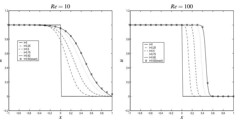
u0(x) =u(x,0) =1, −1≤x≤0, (11) u0(x) =u(x,0) =0, 0<x≤1, (12) where u is velocity, and Re the Reynolds num-ber. Since it is a 1D problem, the differential equation can be solved efficiently, without the need for converting RBF coefficients into nodal values. The IRBFN expressions (2)-(4) can thus be used to represent the variable and its deriva-tives. The space domain is discretised with 101 collocation points. Results for the casesRe=10 andRe=100 are shown in Figure 1 where exce-lent agreement with the exact solution [Fletcher (1984)] can be seen. The “shock” front becomes diffused at lowRevalues and remains steep with increasingRevalues.

4 Lid-driven cavity flow

This is a classical benchmark problem which is suitably used here to demonstrate the capability of the present method to simulate complex fluid flows. The lid velocity (U) and the length of the side of the square (L) are used as reference quantities. The non-dimensional governing equa-tions for unsteady two-dimensional incompress-ible flow of a Newtonian fluid in terms of the streamfunctionψ and vorticityω can be written as follows

∂ω ∂t +

∂ψ ∂x2

∂ω ∂x1−

∂ψ ∂x1

∂ω ∂x2

= 1 Re

∂2_ω ∂x2 1

+∂2ω ∂x2 2

, (13)

∂2_ψ ∂x2₁ +

∂2_ψ

∂x2₂ =−ω, (14)

whereRe=U L/νis the Reynolds number(ν: the kinematic viscosity). The vorticity and stream-function are defined by

ω=∂v2 ∂x1 −

∂v1 ∂x2,

(15) ∂ψ

∂x1 =− v2, ∂ψ

∂x2 =

−1 −0.8 −0.6 −0.4 −0.2 0 0.2 0.4 0.6 0.8 1 −0.2

0 0.2 0.4 0.6 0.8 1 1.2

t=0 t=0.25 t=0.5 t=0.75 t=0.92 t=0.92(exact)

Re=10

x

u

−1 −0.8 −0.6 −0.4 −0.2 0 0.2 0.4 0.6 0.8 1 −0.2

0 0.2 0.4 0.6 0.8 1 1.2

t=0 t=0.25 t=0.5 t=0.75 t=0.92 t=0.92(exact)

Re=100

x

u

Figure 1: Burgers equation, 101 data points,Δt=0.001: the evolution of the “shock” front.

wherev1andv2are two components of the veloc-ity vector in thex1− andx2−directions, respec-tively.

The lid slides toward the right at unit velocity, while the other walls remain stationary:

ψ=0, ∂ψ ∂x1 =

0, on x1=0 andx1=1, (17)

ψ=0, ∂ψ ∂x2

=0, on x2=0, (18)

ψ=0, ∂ψ ∂x2 =

1, on x2=1. (19)

The boundary conditionψ =0 along the bound-aries can be used directly to solve (14) for the ve-locity field, while one needs to derive computa-tional boundary conditions for the vorticity trans-port equation (13). Using (14) and the boundary conditionψ =0, expressions for the vorticity on the boundaries are reduced toω=−∂2ψ/∂n2(n: the local coordinate normal to the wall). After ex-pressing this normal second-order derivative as a linear combination of nodal first-order derivative values, imposition of the required boundary con-ditions∂ψ/∂nis carried out. Finally, the remain-ing first derivative values are written in terms of nodal streamfunction values. This process is sim-ilar to that of a 2D-IRBFN interpolation scheme which was described in detail in [Mai-Duy and

Tran-Cong (2005)]. The present solution proce-dure involves the following steps

1. Guess a set of initial conditions: ω,ψ and their spatial derivatives

2. Discretize in time using a finite-difference scheme,

3. Discretize in space using 1D-IRBFN schemes:

Compute the convective term and the bound-ary values ofω

Solve the vorticity transport equation (13) forω

Solve Poisson equation (14) forψ

4. Check to see whether the solution has reached a steady state

∑N i=1

ψ(i) k+1−ψ

(i) k

2

∑N i=1

ψ(i) k+1

2 <ε, (20)

where k is the time level, ε the tolerance (ε=10−9_{), andNthe number of collocation} points.

T able 1 : L id-d ri v en ca v ity fl o w , Re = 100: Extr em a o f the v er tic al an d hor iz onta l v eloc ity pr ofi le s thr ough the ce n tr e o f the ca vity . M ethod De nsity

v1mi

n (erro r % ) x2 v2ma

x (erro r % ) x1 v2mi

T able 2 : L id-d ri v en ca v ity fl o w , Re = 1000: Extr em a o f the v er tic al an d hor iz onta l v eloc ity pr ofi le s thr ough the ce n tr e o f the ca vity . N ote tha t cpi. : consiste nt physic al inte rpola tion; sta gg. : sta gge re d. M ethod De nsity

v1mi

n (erro r % ) x2 v2ma

x (erro r % ) x1 v2mi

The stability of the lid-driven cavity flow was investigated in [e.g. Poliashenko and Aidun (1995)]. For the case of a square cavity, it was re-ported that the point of bifurcation isRe=7763, where the primary steady state becomes unstable. A range of Re={0,100,400,1000,3200,5000} is considered here. The computed solution at the lower and nearest value of Re is taken to be the initial solution. The special case ofRe=0 starts from a fluid at rest. Ten uniform grids, namely 11×11,21×21,···,101×101, are employed to study the convergence behaviour of the method. Time steps used are in the range of 0.005−0.5. Steady-state solutions are presented in detail here, and they are compared with some other numerical results available in the literature.

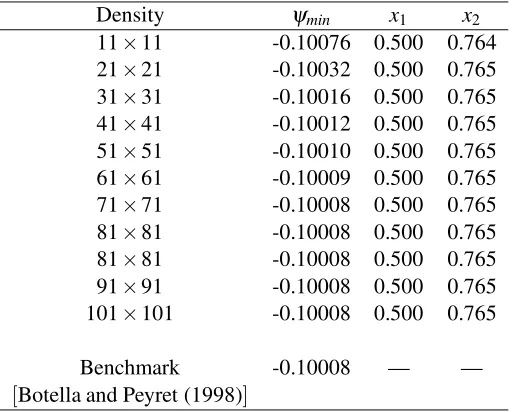
The accuracy of the method is first examined through the solution of the Stokes flow. The gov-erning equation for this creeping flow can be ob-tained from (13) by simply discarding the non-linear term and settingRe equal to 1. The com-puted values of the streamfunction at the centre of the primary vortex are given in Table 5. The spectral results [Botella and Peyret (1998)] are also included to provide the basis for the assess-ment of the accuracy of the present method. A very high degree of accuracy is achieved. When Nx1 =Nx2 ≥71, five significant digits remain un-changed.

For viscous flow (Re>0), results concerning the extrema of the velocity profiles along the ver-tical and horizontal centrelines (Re = 100 and Re=1000), and the intensity of the primary vor-tex and lower right secondary vorvor-tex (Re=1000) are summarized in Tables 1–4. The correspond-ing results obtained by the pseudospectral method [Botella and Peyret (1998)], FDM [Ghia, Ghia, and Shin (1982), Bruneau and Jouron (1990)] and FVM [Deng, Piquet, Queutey, and Visonneau (1994)] are included for comparison. The 1D-IRBFN results are in better agreement with the spectral solutions than those predicted by FDM and FVM.

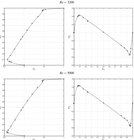
For the case of Re=3200 and Re=5000, ve-locity profiles on the vertical and horizontal lines through the cavity geometric centre are plotted in Figure 2. They compare well with the

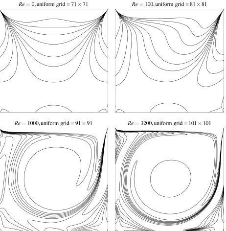
correspond-ing results of Ghia, Ghia, and Shin (1982). In addition, iso-vorticity lines of the flow for various Re numbers are shown in Figure 3. The vorticity-contour values chosen here are the same as those in [Ghia, Ghia, and Shin (1982), Botella and Peyret (1998)], i.e. {-5, -4,-3,-2,-1,-0.5,0,0.5,1,2,3}. The plots look reasonable when compared to those of Ghia, Ghia, and Shin (1982) and Botella and Peyret (1998).

It is worth mentioning that although the present method is global, it does not require any special treatment for the singularity at the two corners. In contrast, when using the spectral collocation method, it is necessary to employ a subtraction technique to remove the leading part of the singu-larity.

For the simulation of the lid-driven viscous flow, the 1D-IRBFN collocation method achieves a very high degree of accuracy using relatively coarse grids.

5 Moving interface problems

The IRBFN method is combined with the level set (LS) method in a scheme, namely IRBFN-LS, to capture the evolution of the interface. In this work, passive transport problems are chosen so that focus is kept on the moving interface.

5.1 Level set method

The underlying idea of the level set method is to embed a moving interfaceΓas the zero level set of a smooth (at least Lipchitz continuous) function φ(x,t)known as the level set function [e.g. Osher and Sethian (1988)]. The moving interface is then captured at all time by locating the set ofΓ(t)for which φ vanishes. The level set function is ad-vected with time by a transport equation which is known as a level set equation. Usually,φis de-fined as a signed distance function to the interface. Readers are referred to [e.g. Sethian (1999), Os-her and Fedkiw (2003)] for detailed discussions on the level set method.

dimen-Re=3200

−00.5 0 0.5 1 0.1

0.2 0.3 0.4 0.5 0.6 0.7 0.8 0.9 1

v1

x2

0 0.1 0.2 0.3 0.4 0.5 0.6 0.7 0.8 0.9 1

−0.8 −0.6 −0.4 −0.2 0 0.2 0.4 0.6

x1

v2

Re=5000

−00.5 0 0.5 1 0.1

0.2 0.3 0.4 0.5 0.6 0.7 0.8 0.9 1

v1

x2

0 0.1 0.2 0.3 0.4 0.5 0.6 0.7 0.8 0.9 1

−0.8 −0.6 −0.4 −0.2 0 0.2 0.4 0.6

x1

v2

Re=0,uniform grid = 71×71 Re=100,uniform grid = 81×81

Re=1000,uniform grid = 91×91 Re=3200,uniform grid = 101×101

Table 5: Lid-driven cavity flow,Re=0: The minimum value of the streamfunction and its location.

Density ψmin x1 x2

11×11 -0.10076 0.500 0.764 21×21 -0.10032 0.500 0.765 31×31 -0.10016 0.500 0.765 41×41 -0.10012 0.500 0.765 51×51 -0.10010 0.500 0.765 61×61 -0.10009 0.500 0.765 71×71 -0.10008 0.500 0.765 81×81 -0.10008 0.500 0.765 81×81 -0.10008 0.500 0.765 91×91 -0.10008 0.500 0.765 101×101 -0.10008 0.500 0.765

Benchmark -0.10008 — —

[Botella and Peyret (1998)]

sional functionφ(x,t) Γ(t) ={x∈Rd|φ(x,t) =0}.

Initially,φ is defined as the signed distance func-tion from the front such that

φ(x,t) =

⎧ ⎨ ⎩

+d(x,t) x∈Ω+, 0 x∈Γ,

−d(x,t) x∈Ω−,

(21)

where d(x,t) represents the Euclidean distance from x to the interface,Ω− andΩ+ are interior and exterior regions, respectively. The interface can be then captured at any time by locating the set ofΓ(t)for whichφ vanishes. In other words, instead of working with the interface, one evolves the level set with the following transport equation forφ,

φt+v·∇φ=0, (22)

φ(x,0) =φ0, (23)

whereφ0 is a given function. Whenever needed, the moving interface can be extracted as the zero level of the level set functionφ. Interested read-ers are referred to [e.g. Osher and Sethian (1988), Sethian (1999), Osher and Fedkiw (2003)] for fur-ther details.

5.2 IRBFN-LS scheme

Consider a two-dimensional material interface moving with an externally generated velocity

field. The IRBFN-LS scheme for capturing the interface is described by the following steps

1. Initialize the level set functionφ(x)to be the signed distance to the interface as described by equation (21);

2. Update the externally generated velocity field using the current value of the level set function. For Newtonian fluid flows, this in-volves solving the Navier-Stokes equations by methods such as the one is discussed in section 2. For passive transport problems, the external velocity field simply remains un-changed;

3. Solve the level set equation (22) by the method of lines for one time step using the newly updated velocity field from step 2;

4. Re-initialize the level set function that has just been calculated from the previous step to a signed distance function;

5.3 Initialization

At timet=0, the signed distance function in (21) is defined as the distance from the given colloca-tion pointx to the initial interface curve and the sign is chosen to be positive if the point is inside the curve, and negative if outside:

d(x,0) =±minx−x(i), x(i)∈Γ0, (24)

whereΓ0=Γ(0)is the initial interface whose dis-crete representation isx(i).

5.4 Method of lines

The level set equation is solved in the IRBFN framework. Using the method of lines, one can convert the PDE (22) into a first-order initial-value system of ODEs. Spatial derivatives, i.e. ∂φ/∂xj, are discretized by means of 2D-IRBFNs. Solving the obtained ODE system with the initial conditions (23) yields the level set function at ev-ery data point within the time interval of interest.

5.5 Re-initialization

While the level set functionφ is initialized as a signed distance function from the moving inter-face, this is not necessarily true as time proceeds. In order to keep the numerical solution accurate, one needs to reinitialize φ to be the signed dis-tance function from the evolving front Γat each time step. The basic idea behind this scheme of re-initialization is that given a functionφ(x) that is not a distance function, one can evolve it into a function φ that is exact signed distance func-tion from the zero level set of φ(x) [e.g. Suss-man, Smereka, and Osher (1994)]. This is ac-complished by solving the following problem to steady state

φt =Sε(φ) (1−|∇φ|) (25) φ(x,0) =φ(x), (26)

whereS_ε denotes the smoothed sign function

S_ε(φ) = φ φ2+ε2

, (27)

where ε can be chosen to be the minimum dis-tance from any data point to the others.

The solution procedure for(25)-(27)is similar to that of (22)-(23). It should be noted that because the level set function is reinitialized at each time step, the steady solution of (25) can be obtained after just a small number of iterations [e.g. Suss-man, Smereka, and Osher (1994)].

5.6 Numerical examples

5.6.1 Solid body rotation

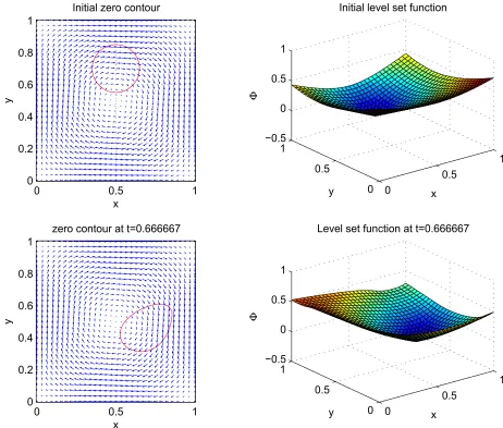
Consider the solid body rotation of a circular bub-ble of radius r=1 centered at(−1,0) in a vor-tex flow with velocity field(v1,v2) = (−x2,x1). A half cycle of rotation is performed, and the per-centage change in area of the circle during its mo-tion is measured. As can be seen from Table 6, the meshless IRBFN-LS scheme yields more accurate solutions with coarser point density in compari-son with the mesh-based level set method [Sethian (1999)]. Figure 4 shows the zero contours of the level set function at different points in time dur-ing the rotation of the circle. In this figure, the computational grid consists of 41 ×41 colloca-tion points and the time step size is chosen to be 0.0125. As can be seen from the figure, the mov-ing interface is well captured and reconstructed by the IRBFN-LS method.

5.6.2 Circular bubble moving in shear flow

Consider a circular bubble of radiusr=0.15, ini-tially centered at(0.5,0.7)moving by a shear flow in a cavity of size[0,1]×[0,1]with the velocity field(v1,v2)defined as follows

v1 = −sin(πx1)cos(πx2), (28) v2 = cos(πx1)sin(πx2). (29)

With such velocity field, the bubble is passively transported in forms of rotation and stretching. The IRBFN-LS scheme is used to capture the moving interface with time in a computational grid of 65×65. The time step sizeΔtin the semi-discrete scheme for solving the level set equation is chosen following the multidimensional CFL condition [Osher and Fedkiw (2003)]

Δt max

|v1| Δx1+

|v2| Δx2

Table 6: Solid body rotation: Comparisons between the mesh-based LSM [Sethian (1999)] and the IRBFN-LS method on the percentage change in area att=1.

Grid size 1st_{-order mesh-based LSM 2}nd_{-order mesh-based LSM IRBFN-LS}

21×21 51.88% 18.00% 1.6275%

41×41 37.981% 2.276% 0.3987%

−1.5 −1 −0.5 0 0.5 1 1.5

−1.5

−1

−0.5 0 0.5 1 1.5

0 0.5 1 0

0.2 0.4 0.6 0.8 1

x

y

Initial zero contour

0

0.5

1

0 0.5

1 −0.5 0 0.5 1

x Initial level set function

y

Φ

0 0.5 1

0 0.2 0.4 0.6 0.8 1

x

y

zero contour at t=0.666667

0

0.5

1

0 0.5

1 −0.5 0 0.5 1

x Level set function at t=0.666667

y

Φ

Figure 5: Circular bubble moving in shear flow: Zero contour and the level set function att=0 andt= 0.666667 during the rotation of a circle.

where α is the CFL number, 0< α <1 and α=0.5 for this example;|v1|and|v2|are the ab-solute values of normal and tangential velocity; Δx1 andΔx2are grid density in thex1−andx2− directions, respectively. In this example, the time step size is 0.0078125. Figure 5 shows the level set function and the moving interface as its zero level at different points in time during the rotation of the circle. Reinitialization is performed after each time step with 5 iterations for the level set function to be a signed distance function. Numeri-cal experiments are carried out with the number of steps greater than 1 where the reinitialization pro-cess is performed, and it is found that, although more computational work is needed,

reinitializa-tion after each time step yields more stable results.

6 Concluding remarks

0 0.5 1 0

0.2 0.4 0.6 0.8 1

x

y

zero contour at t=1.70833

0

0.5

1

0 0.5

1 −0.5 0 0.5 1

x Level set function at t=1.70833

y

Φ

0 0.5 1

0 0.2 0.4 0.6 0.8 1

x

y

zero contour at t=2.91667

0

0.5

1

0 0.5

1 −0.5 0 0.5 1

x Level set function at t=2.91667

y

Φ

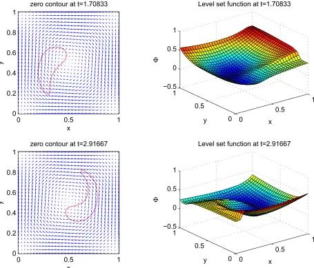
Figure 6: Circular bubble moving in shear flow: Zero contour and the level set function att=1.70833 and t=2.91667 during the rotation of a circle.

top corners. For moving interface problems, the present scheme combines the highly accurate ap-proximator coming from the IRBFN method with the advantage of the level set method in dealing quite naturally with the moving interface as the zero contour of a smooth function. It can be seen from the examples that the evolution of the mov-ing interface is captured very well by the present scheme.

Acknowledgement: L. Mai-Cao is supported by a USQ scholarship, USQ Faculty of Engineer-ing and SurveyEngineer-ing scholarship and a Moldflow scholarship.

References

Botella, O.; Peyret, R. (1998): Bench-mark spectral results on the lid-driven cavity flow. Computers & Fluids, vol. 27, pp. 421–433.

Bruneau, C.-H.; Jouron, C.(1990): An ef-ficient scheme for solving steady incompressible Navier-Stokes equations. Journal of Computa-tional Physics, vol. 89, pp. 389–413.

Deng, G.; Piquet, J.; Queutey, P.; Visonneau, M. (1994): Incompressible flow calculations with a consistent physical interpolation finite vol-ume approach. Computers & Fluids, vol. 23, pp. 1029–1047.

Fletcher, C.(1984): Computational Galerkin Methods. Springer-Verlag, New York.

Floryan, J.; Rasmussen, H.(1989): Numerical Methods for Viscous Flows with Moving Bound-ary. Applied Mechanics Reviews, vol. 42, pp. 323–341.

Ghia, U.; Ghia, K.; Shin, C. (1982): High-Re solutions for incompressible flow using the Navier-Stokes equations and a multigrid method. Journal of Computational Physics, vol. 48, pp. 387–411.

Hon, Y.; Ling, L.; Liew, K.(2005): Numerical analysis of parameters in a laminated beam model by radial basis functions. CMC: Computers, Ma-terials & Continua, vol. 2, pp. 39–50.

Kansa, E. (1990): Multiquadrics- A scat-tered data approximation scheme with applica-tions to computational fluid-dynamics-II. Solu-tions to parabolic, hyperbolic and elliptic partial differential equations. Computers and Mathemat-ics with Applications, vol. 19, pp. 147–161.

La-Rocca, A.; Power, H.; La-Rocca, V.; Morale, M. (2005): A meshless approach based upon radial basis function hermite collo-cation method for predicting the cooling and the freezing times of foods. CMC: Computers, Ma-terials & Continua, vol. 2, pp. 239–250.

Mai-Cao, L.; Tran-Cong, T.(2005): A Mesh-less IRBFN-Based Method for Transient Prob-lems. CMES: Computer Modeling in Engineer-ing & Sciences, vol. 7, pp. 149–171.

Mai-Duy, N. (2004): Indirect RBFN method with scattered points for numerical solution of PDEs. CMES:Computer Modeling in Engineer-ing & Sciences, vol. 6, pp. 209–226.

Mai-Duy, N.; Tran-Cong, T.(2001a): Numer-ical solution of differential equations using

mul-tiquadric radial basis function networks. Neural Networks, vol. 14, pp. 185–199.

Mai-Duy, N.; Tran-Cong, T. (2001b): Nu-merical solution of Navier-Stokes equations us-ing multiquadric radial basis function networks. International Journal for Numerical Methods in Fluids, vol. 37, pp. 65–86.

Mai-Duy, N.; Tran-Cong, T.(2003): Approxi-mation of function and its derivatives using radial basis function networks. Applied Mathematical Modelling, vol. 27, pp. 197–220.

Mai-Duy, N.; Tran-Cong, T.(2005): An effi-cient indirect RBFN-based method for numerical solution of PDEs. Numerical Methods for Partial Differential Equations, vol. 21, pp. 770–790.

Osher, S.; Fedkiw, R. (2003): Level Set Methods and Dynamic Implicit Surfaces, Applied Mathematical Sciences (Vol 153). Springer, New York.

Osher, S.; Sethian, J.(1988): Fronts propagat-ing with curvature-dependent speed: algorithms based on Hamilton-Jacobi formulations. Journal of Computational Physics, vol. 79, pp. 12–49.

Poliashenko, M.; Aidun, C.(1995): A direct method for computation of simple bifurcations. Journal of Computational Physics, vol. 121, pp. 246–260.

Sarler, B.(2005): A radial basis function col-location approach in computational fluid dynam-ics. CMES: Computer Modeling in Engineering & Sciences, vol. 7, pp. 185–194.

Sethian, J.(1999): Level Set Methods and Fast Marching Methods: Evolving Interfaces in Com-putational Geometry, Fluid Mechanics, Computer Vision, and Materials Science. Cambridge Uni-versity Press, New York.

Sussman, M.; Smereka, P.; Osher, S. (1994): A level set approach for computing solutions to incompressible two-phase flow. Journal of Com-putational Physics, vol. 114, pp. 146–159.

Tolstykh, A.; Shirobokov, D. (2005): Us-ing radial basis functions in a “finite difference mode”. CMES: Computer Modeling in Engineer-ing & Sciences, vol. 7, pp. 207–222.