Theses
8-2018
An Empirical Evaluation of the Indicators for
Performance Regression Test Selection
Kevin Hannigan
Follow this and additional works at:https://scholarworks.rit.edu/theses
This Thesis is brought to you for free and open access by RIT Scholar Works. It has been accepted for inclusion in Theses by an authorized administrator of RIT Scholar Works. For more information, please [email protected].
Recommended Citation
Indicators for Performance Regression
Test Selection
by
Kevin Hannigan
A Thesis Submitted in Partial Fulfillment of the
Requirements for the Degree of
Master of Science in Software Engineering
Supervised by
Dr. Mohamed Wiem Mkaouer
Department of Software Engineering
B. Thomas Golisano College of Computing and Information Sciences
Rochester Institute of Technology
Rochester, New York
nation Committee:
Dr. Mohamed Wiem Mkaouer Assistant Professor
Thesis Committee Chair
Dr. Christian D. Newman Assistant Professor
Dr. J. Scott Hawker Associate Professor
As a software application is developed and maintained, changes to the source code may
cause unintentional slowdowns in functionality. These slowdowns are known as
perfor-mance regressions. Projects which are concerned about perforperfor-mance oftentimes create
performance regression tests, which can be run to detect performance regressions. Ideally
we would run these tests on every commit, however, these tests usually need a large amount
of time or resources in order to simulate realistic scenarios.
The paper entitled ”Perphecy: Performance Regression Test Selection Made Simple but
Effective” presents a technique to solve this problem by attempting to predict the likelihood
that a commit will cause a performance regression. They use static and dynamic analysis to
gather several metrics for their prediction, and then they evaluate those metrics on several
projects. This thesis seeks to replicate and expand on their work.
This thesis aims in revisiting the above-mentioned research paper by replicating its
experiments and extending it by including a larger set of code changes to better understand
how several metrics can be combined to approximate a better prediction of any code change
that may potentially introduce deterioration at the performance of the software execution.
This thesis has successfully replicated the existing study along with generating more
insights related to the approach, and provides an open-source tool that can help developers
Abstract . . . .
1 Introduction. . . 1
2 Research Objective . . . 4
2.1 Motivation . . . 4
2.2 Contribution . . . 5
2.3 Research Questions . . . 6
3 Related Work . . . 7
4 Perphecy . . . 8
4.1 Summary . . . 8
5 Methodology . . . 11
5.1 Data Collection . . . 11
5.2 Data Analysis . . . 12
5.2.1 Determining Significant Changes . . . 12
5.2.2 Determining the Indicator Metrics . . . 13
5.2.3 Determining Thresholds . . . 15
6 Analysis & Discussion . . . 17
6.1 RQ1: What predictors does the Perphecy approach generate when used on a larger dataset? . . . 17
6.1.1 What is the potential for any test selection technique? . . . 17
6.1.2 Generating and Evaluating the Predictors . . . 18
6.2 RQ2: What are the most useful indicators when considered independently? 20 7 Threats to Validity . . . 25
4.1 Indicator Descriptions and Rationales . . . 9
5.1 Example indicator results . . . 13
6.1 Hit and Dismiss Rates for the three different predictors . . . 19
2.1 Example execution times . . . 5
5.1 Perphecy Threshold Algorithm . . . 15
6.1 Indicator 1 - Del Func≥X . . . 21
6.2 Indicator 2 - New Func≥X . . . 22
6.3 Indicator 3 - Reached Del Func≥X . . . 22
6.4 Indicator 4 - Top Chg by Call≥X% . . . 23
6.5 Indicator 5 - Top≥X% by Call Chg by≥10% . . . 23
6.6 Indicator 7 - Top Chg Len≥X% . . . 24
Chapter 1
Introduction
For many software projects, performance is a critical requirement. Such projects often
create performance tests alongside their other tests which specifically test for performance
bugs. Performance bugs are often problems with slow execution time, though other
quali-ties like memory usage can be considered too [10].
Performance tests come with some unique constraints as opposed to automated unit
testing. For performance tests to work, they typically need to use many resources, run for a
long time, or execute demanding functionality, because they require a realistic scenario in
order to operate. Ideally performance tests could be run for every commit, perhaps as part
of a continuous integration system, similar to having your unit tests run on every commit.
However, this is usually too expensive and time consuming to implement [2, 3].
Practically, as software evolves, a continuous set of code changes is being introduced,
within each, one or few changes may be responsible for introducing slowdowns or speedups
to the current system’s execution. This is known as a performance regression. Performance
regression defines any unexpected system performance in terms of runtime, when compared
to its previous state, before the change, for the same set of input values, and for the same
type of behavior (functional scenarios). Thus, developers are eager to detect any code
changes that accidentally introduces such significant slower runtime.
Detecting code changes responsible for performance regression is challenging due to
the rapidity of software evolution i.e., the number of committed changes is increasing on
a daily basis [4]. And so, it is hard to individually monitor these changes while being
separately test each code change for all possible functional test cases. Furthermore, some
changes may not directly reflect performance issues since they may be only triggered by
special cases (for specific type of users or workloads) and so, they may be detected later
in the testing process once other changes have been also committed. So, there is a need
of introducing better techniques in predicting whether a given change can be potentially
hazardous to the system’s performance [12].
Existing studies try to solve this issue by predicting whether or not a commit will cause
a regression to occur. The hope is that by creating a system that can successfully evaluate
the need to run the performance tests on a change, we can reduce the number of times
we run the tests, and thus save cost. The paper ”Perphecy: Performance Regression Test
Selection Made Simple but Effective” [9] presents a system that predicts whether or not a
commit will cause a performance regression. Their system works by looking at 8 metrics,
to predict for each benchmark whether or not a significant performance change will occur.
They look at 4 different projects, for a total of 429 commits. They use metrics called hit
rate (the percent of correct predictions of a performance regression) and dismiss rate (the
percent of correct predictions that a regression will not occur) to evaluate their system’s
performance.
The 8 indicators are discussed in detail in Chapter 4, Perphecy. However, to help
il-lustrate this, consider the following example. In listing 1.1, two excerpts from a diff are
shown. One of the metrics used in the study is based on the percent function length change.
In the first block in the example, we see that three lines from the function are deleted. The
percent static function length change, therefore, is 50%. In the second block, one line of
code is changed, but not added or removed. In this case, the static function length change
is 0%. However, a different metric could be affected, such as ”Highest percent overhead
function changed”, if this one line edit happened in a frequently called function.
Perphecy takes the calculated metrics and compares them to a predetermined threshold
value. The metrics and their thresholds are called an ”indicator” in the Perphecy paper. As
consider. The collection of indicators is called a predictor. If any of the thresholds of the
indicators in the predictor are exceeded, Perphecy predicts that a regression will occur. So,
in this example, if we had these two blocks edited between commits, If the predictor that
Perphecy had determined included ”static function length change”, and the threshold was
40%, Perphecy would predict a regression. Contrarily, if the threshold was 60%, it would
not predict a regression unless one of the other indicators in the predictor was affected.
Listing 1.1: Descriptive Caption Text
static intgitdiff_oldname(const char*line, struct patch *patch) {
- char*orig = patch->old_name;
patch->old_name = gitdiff_verify_name(line, patch->is_new, patch->old_name, DIFF_OLD_NAME);
- if(orig != patch->old_name) - free(orig);
return 0; }
@@ -459,7 +462,7 @@static int get_urlmatch(const char*var,const char*url) free(config.url.url);
free((void*)config.section);
- return 0;
+ return ret;
}
The Perphecy paper, however, has a few limitations. First, their dataset was fairly small.
As an example, one of the projects they ran on was git. They ran 5 tests on approximately
200 commits, and found 13 cases of regressions. This is a small sample size to base
con-clusions off of. Second, they did not show the final set of indicators that were used to give
their results. They only show the method of how they obtained them.
In this paper, we attempt to replicate this study. We look at one of the studied projects:
Git. We study 8596 of the more recent commits from the project, significantly more than
the 201 studied in the paper. We present insights about the original study, such as a flaw in
the original threshold selection algorithm and our mitigation, a more thorough analysis of
the potential of each individual indicator, and the results of the predictor that was generated
Chapter 2
Research Objective
2.1
Motivation
Executing tests on every software change is a popular practice in Continuous Integration,
with numerous benefits, namely the fast and continual detection of bugs throughout the
development lifecycle. Performance tests, however, can not practically be run this way
because it would be too expensive. The goal of this area of research is to develop techniques
which decrease the cost of performance testing, while still decreasing the time it takes for
developers to get feedback about whether their code has performance bugs or not.
The Perphecy study makes steps towards building a system that can predict whether
a change will cause a performance regression or not. A system like that can help limit
which commits need to be tested, which can save cost. If a system could be created which
very reliably could predict whether a performance bug would occur or not, it could be used
entirely in place of running the tests periodically, and would spend an optimal amount of
time running performance tests.
A performance regression, in the context of this paper, is defined as anytime a test’s
execution time is longer than for the previous commit’s in a statistically significant way.
In the original paper, and in this one, we identify statistically significant regressions by
taking 5 samples of the execution times for each commit and performing a t-test between
every two commits. In figure 2.1, we show an example of these execution times. In this
case, though it may be small, the t-test determined that there was a regression from commit
Figure 2.1: Example execution times
2.2
Contribution
Our main contribution is to replicate and extend the Perphecy paper. Our main contributions
are:
1. Scalability. Since performance regression can be linked to various aspects of code
changes, it is important to diversify the set of possible types of changes that may
trigger situations in which the software performance deteriorates. For that reason,
we examine, in this thesis, a larger dataset compared to the original study.
2. Prediction. The original study outcome was the generation of a predictor that
accu-rately predicts the occurrence of a performance regression, for a given set of code
changes. This predictor is constructed using an automatically generated combination
of tuned indicators and metrics. This generation of the combination of indicators
generated predictors. Thus, we explore the combination of indicators for a different
set of changes in order to demonstrate how the predictor is generated and provide
more details about its combination.
3. Indicators. The indicators represent the building block of the predictor and so they
are important in providing good prediction results, if the set of used indicators can
cover all the possible performance aspects. In this context, we explore the statically
and dynamically calculated indicators in terms of their performance in constructing
good indicators.
2.3
Research Questions
We revisit the Perphecy experiment to further elaborate on these questions:
• RQ1:What predictors does the Perphecy approach generate when used on a larger
dataset? In the Perphecy paper, they don’t give the actual predictors (combination of
indicators and thresholds) that were generated, only the hit and dismiss rates that the
predictor gave.
• RQ2: What are the most useful indicators when considered independently? For
our dataset, which of the indicators has the best combination of hit and dismiss rates
Chapter 3
Related Work
Regression Test Selection has been studied previously in many different papers . The most
relevant work is the study of regression test selection. However, this research has usually
been focused on correctness tests, like unit tests, rather than performance.
A study by Luo et al, ”Mining Performance Regression Inducing Code Changes in
Evolving Software”, [6] investigates how to identify the code changes that induced a
per-formance regression. The tool they create, PerfImpact, works by searching for input
combi-nations to a program which are likely to lead to a performance regression, and then profiling
the execution trace when using those inputs to estimate the impact of past code changes on
the detected regression. Using execution traces / dynamic profile information as they do in
this paper is a key part of the indicators used in the Perphecy study.
Alcocer et al [1] study what kinds of source code changes are responsible for
mance regressions in open source software. They determine if a commit causes a
perfor-mance variation with static analysis and dynamic analysis. They also show that they can
get good results without running dynamic profiling for every change.
One similar study by Huang et al. [5] looks into what they call Performance Risk
Analysis, or PRA. They use static analysis to estimate how expensive each function is
by looking at function length, loops, and known expensive functions. Through this static
analysis of a function’s ”expensiveness”, they predict the risk that a change will cause a
regression. Their analysis showed they could catch 87%-95% of regressions by testing
Chapter 4
Perphecy
4.1
Summary
Perphecy is a system which ”predicts if a code commit will affect the performance of a
benchmark in a benchmark suite”. Given a ”before” commit, an ”after” commit, and a
performance test (also called a benchmark), Perphecy will predict whether or not that test
will experience a performance regression from one commit to the other. By collecting
metrics about the source code through both static and dynamic analysis, the authors of
Perphecy found they were able to save as much as 83% of benchmarking time while still
detecting 85% of performance affecting code changes.
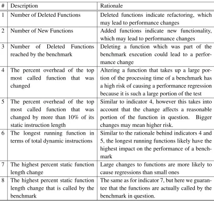
Perphecy uses 8 metrics which they distill into what they call ”Indicators”. The
indi-cators are determined to be true or false by comparing to a static threshold, which they
determined using a greedy algorithm that I will explain later. Each indicator is calculated
specifically for each ”old commit, new commit, benchmark” triplet that needs to be
con-sidered. These indicators, along with the rationale for each, are included below, in Table
4.1.
In order to calculate the metrics, both static and dynamic analysis is needed. Perphecy’s
solution for getting the dynamic results is to do a separate run of the performance tests with
the dynamic analysis tool active, anytime it predicts a regression. When calculating the
metrics, the most recent available dynamic analysis data for the benchmarks is used. Over
time though, it is certainly possible for this information to get out of date.
Table 4.1: Indicator Descriptions and Rationales
# Description Rationale
1 Number of Deleted Functions Deleted functions indicate refactoring, which
may lead to performance changes
2 Number of New Functions Added functions indicate new functionality,
which may lead to performance changes
3 Number of Deleted Functions
reached by the benchmark
Deleting a function which was part of the benchmark execution could lead to a perfor-mance change
4 The percent overhead of the top
most called function that was changed
Altering a function that takes up a large por-tion of the processing time of a benchmark has a high risk of causing a performance regression because it is such a large portion of the test
5 The percent overhead of the top
most called function that was changed by more than 10% of its static instruction length
Similar to indicator 4, however this takes into account that the change affects a reasonable portion of the function in question. Bigger changes may mean higher risk.
6 The longest running function in
terms of total dynamic instructions
Similar to the rationale behind indicators 4 and 5, the longest running functions likely have the highest impact on the performance of a bench-mark
7 The highest percent static function length change
Large changes to functions are more likely to cause regressions than small ones
8 The highest percent static function length change that is called by the benchmark
The same as for indicator 7, but here we guaran-tee that the functions are actually called by the benchmark in question.
meant by ”longest running function by total dynamic instructions”, but we could interpret
it two ways. Either they were referring to the total number of instructions executed in that
function over the course of the entire benchmark, or they were referring to the average
number of instructions executed by the function each time it was called - the average
dy-namic instruction length. If the former was true, this is effectively the same as indicator
4. Multiplying the percent overhead by the total number of instructions executed in the
number would be in perfect ratio relative to the other functions in the benchmark, and we
only compare the functions to each other, so there would be no effective difference between
these indicators. On the other hand, if the latter interpretation is true, it was unclear to us
how to determine the average dynamic instruction length using the tool recommended
-perf. Indicator 8 is similar, but it uses static function length instead of average dynamic
function instruction count. While it is a limitation that we were unable to replicate the
results of indicator 6, we believe that the other indicators provide sufficient coverage to
Chapter 5
Methodology
5.1
Data Collection
Replicating the study required first collecting all of the necessary data. There were three
kinds of data needed: - Results of running each performance test - Static information for
the indicators - List of functions and their start and end line in the source code - Dynamic
information for the indicators - Function overhead percentage for each benchmark
We collected data for 8798 commits originally. Those commits were chosen by
exe-cuting the ‘git rev-parse‘ command from the master branch at the time and going back to
the first commit we could find which had performance tests. Across that range of commits,
there were were 202 commits which, for various reasons, did not have any tests, so we
removed them. Thus in total we considered 8596 commits.
Running all of the performance tests for a single commit takes a long time (hence the
need for this study) so we parallelized the task across many machines. The results of the
git performance tests are reported in wall time, which can be impacted by using different
machines with different clock speeds, RAM, and such, so to mitigate this we used identical
DigitalOcean virtual machine servers. These virtual servers were the standard DigitalOcean
Ubuntu 16.04 x64 droplets with 1 CPU clocked at 2.2GHz and 1GB of RAM. Even after
taking these precautions, there can be noise in the data. To deal with this, we ran each test
five times, which is the same number of runs used in the original study.
The dynamic information was collected using linux perf which was used for some of
case though, the similarity of the machines is not very important because we only look at
which instructions are executed, which should be largely identical, especially if run on the
same operating system.
The static info - the list of functions and their location in the source code - was collected
by using the python lizard tool. While intended for calculating cyclomatic complexity, it
easily gave us a full list of functions identified in all of the source files in the repo for that
commit.
Note that all the data we gathered here is independent of the order of the commits. At
this point we did not calculate the number of functions deleted between two commits, but
rather the list of functions that existed in each commit. Because of this, and because of how
git source control works, we could technically compare commits which were not actually
developed one after the other and see whether or not the tool could predict a regression,
and validate whether the performance was in fact different from commit to commit. We
did not take advantage of this for the most part, but we discuss why this property is useful
in the Threats and Limitations section of the paper.
5.2
Data Analysis
Analyzing the data happened in several stages. First, we determined which commits and
tests experienced a performance regression. Second, we calculated the indicator metrics
for each test in each pair of commits. Once we had that data, we determined the optimal
thresholds for each metric using the greedy algorithm given in the original paper.
5.2.1
Determining Significant Changes
The first step was to determine the truth values for the experiment. If our tool worked
perfectly, what should it predict? For the 8596 commits that we ran on, we went through
each consecutive pair and for each pair, we performed a t-test with an alpha value of 0.05
between the two sets of results. If the t test showed a significant difference between the
then we declared that to be a regression for that benchmark.
5.2.2
Determining the Indicator Metrics
The indicator metrics are the numbers that matter for each of the 8 indicators used in the
original paper. Unfortunately, we were unable to collect the data needed to replicate the
6th indicator from the original paper, ”Top Chg by Instruction”, using the perf tool.
As mentioned before, the values were calculated for every (commit, commit,
bench-mark) triplet that we ran. We used all of the data from the Data Collection stage to calculate
these numbers.
The metrics for each indicator are given below:
1. Number of deleted functions
2. Number of new functions
3. Number of deleted functions reached by the benchmark
4. The highest percent called function for the benchmark that was changed
5. The highest percent called function for the benchmark that was changed by more
than 10% of its static length
6. Not Collected
7. The highest percent of static function length change across all functions
8. The highest percent static function length change for all functions called by the
benchmark
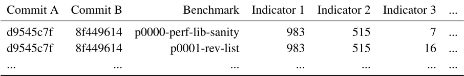
[image:21.612.93.546.601.676.2]This resulted in 176,667 results in a csv file which looked like the results in Table 5.1:
Table 5.1: Example indicator results
Commit A Commit B Benchmark Indicator 1 Indicator 2 Indicator 3 ...
d9545c7f 8f449614 p0000-perf-lib-sanity 983 515 7 ...
d9545c7f 8f449614 p0001-rev-list 983 515 16 ...
Note that these metrics are calculated assuming that dynamic profile data is available for
every commit. This is the optimal situation because it has up to date data for every commit
pair and benchmark. However, as described in the original paper, a dynamic profile would
only be run if a hit was predicted. This would mean the dynamic data slowly becomes out
of date as dismisses are accumulated.
Also note that when considering the dynamic profiling data for indicators 4 and 5, we
5.2.3
Determining Thresholds
Once we had the indicator metrics calculated, we analyzed them to find thresholds using
the approach in the paper. We sampled different threshold values in the range of 0 - 100
for each metric, and generated some graphs showing the hit and dismiss rates for each
threshold value. We show one of these graphs for each indicator in our Analysis Section
[image:23.612.274.513.257.648.2]for Research Question 2.
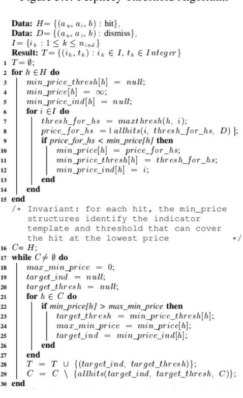
Figure 5.1: Perphecy Threshold Algorithm Our next step was to
repli-cate the algorithm which the
orig-inal paper used to determine the
thresholds. The original algorithm
is shown in Figure 5.1.
We did so, and realized that
there is in fact a problem with the
algorithm the paper used. The
au-thors wrote a basic greedy
algo-rithm which, to summarize in one
sentence, looks at each of the hits,
and finds the minimum
disjunc-tion of indicators which would
have a hit rate of 1.0 with the best
dismiss rate.
However, if a single hit entry
has zero values for all indicators,
due to how the algorithm is
writ-ten, the first indicator it chooses
while trying to create a predictor
will be any indicator with a threshold of 0. A threshold of 0 trivially marks all commits as
Thus, with this algorithm and our data as is, the system marks every commit as a hit, which
is essentially the same as if the system had never been run in the first place.
The basic issue with the greedy approach still applies if only some of the indicators are
zero and one of the indicators is very small. If for example, you have a row where every
indicator metric value is set to 0, except for ”Del Func” which is set to 1, then the algorithm
will pick that Del Func indicator and will wind up hitting a very large number of commits.
Due to this issue, we experiment with filtering out results with all-zero values and result
with any-zero values. We show a comparison of the generated predictors in the next section.
It may seem potentially unlikely for a regression to occur when all of the indicators
are zero values, but one theoretical example would be if a development team updated the
version of a third party framework in a commit. If the framework caused a regression, the
Chapter 6
Analysis & Discussion
In this chapter, we discuss the results of the study and the answers to our research questions.
6.1
RQ1: What predictors does the Perphecy approach
generate when used on a larger dataset?
6.1.1
What is the potential for any test selection technique?
Before we talk about the performance of the predictors that Perphecy generates, we should
put down a few statistics about the gathered data, to help characterize the data and manage
our expectations.
We ran on 8596 commits. Over time, tests were added and removed to the suite of
performance tests, but in general our range of commits begins with 11 tests and ends with
29 commits. Those tests are broken up into subtests, and the test result data is reported for
each subtest in terms of minutes, seconds, and milliseconds it took to complete the tasks.
We summed the subtest times to get a time duration for the test itself.
In all, looking at every combination of commit, commit, benchmark, we had 176,667
”commit, commit, benchmark” results to consider. Of those, 171,656 were dismisses,
ap-proximately 97%. Thus, there were 5011 hits, or 2.84%. This seems to be in line with the
results of the paper - there are proportionally very few commits that involve a significant
performance regression.
Additionally worth note, there were 152,110 rows which contained an indicator metric
a value of 0. This means that for more than half of our ”commit, commit, benchmark”
changes, no functions were added or deleted, the static instruction length of any function
was unchanged, and no function that was more than .01% of the overhead for the
bench-mark was changed. This seemed surprisingly large, but the vast majority of these commits
were either documentation changes, updates to unit tests, or involved things like changing
indentation or tweaking function calls, which do not impact static function length. These
findings tell us that not only do most commits not contain contain a performance
regres-sion, many are trivial changes that have no way of impacting performance tests, and many
are small enough edits in non-critical sections of code that our indicators cannot pick them
up.
Within the 97,420 results which had indicator metric values of all zeros, 1184 rows
(approx. 1.2% of the ”all-zero” rows, and approx. 0.6% of all the rows) were actually
registered as hits! Most of these changes were still of the trivial type - documentation
changes, small one line edits, and the like. We attribute most of these results to noise in
our data collection, however we keep them as part of our dataset because it is perfectly
plausible for changes with no effect on our indicators to impact performance - for example,
if a 3rd party library was updated, and the new version of that library causes a performance
regression.
6.1.2
Generating and Evaluating the Predictors
In order to generate the predictor, we calculated the metrics for the indicators for each
of our commit, commit, benchmark results, then ran the Perphecy threshold algorithm to
output a predictor. As discussed in the Methodology section, we uncovered a problem with
the original algorithm as written. So, when we ran our implementation on the 176,667
”commit, commit, benchmark” rows, the predictor was {Del Func ≥X: 0 }. This will
trivially mark every commit as a hit, giving a Hit Rate of 1.0 and a Dismiss Rate of 0.
To get around this, we tried two changes. First, we tried removing all the entries from
Del Func ≥ X: 1, New Func ≥ X: 1 } (Still fairly trivial). Second, we tried removing
all entries for which anyvalue for the indicators was 0. This gave us the most interesting
predictor: {New Func≥X: 44, Top Chg by Call≥X%: 8%, Reached Del Func≥X: 2,
Top Reached Chg Len ≥X%: 14%, Top Chg Len≥X%: 500%} . Remember that these
different values are handled as a disjunction; if any of these thresholds are met, we predict
a hit for a performance regression.
We evaluated each of these predictors on the three different subsets of our data (the one
with all values, the one with the rows with only zero values removed, and the one with any
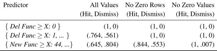
[image:27.612.118.500.321.411.2]rows that had a single zero value removed). The results are shown in Table 6.1.
Table 6.1: Hit and Dismiss Rates for the three different predictors
Predictor All Values No Zero Rows No Zero Values
(Hit, Dismiss) (Hit, Dismiss) (Hit, Dismiss)
{Del Func≥X: 0} (1, 0) (1, 0) (1, 0)
{Del Func≥X: 1, ...} (.764, .561) (1, 0) (1, 0)
{New Func≥X: 44, ...} (.645, .804) (.844, .553) (1, .007)
Some interesting things to point out about these results:
• The predictor generated with all the values is, of course, trivial for all subsets
• The other two predictors have hit rates of 1 for their training set and any subsets of
their training set. However, they also have dismiss rates equal or close to 0 for their
training sets / subsets, which is much different than the results in the paper. When
evaluating their predictor for git on the Full set of their data, they had a hit rate of 1
and a dismiss rate of .83.
• For the other two predictors, their performance on the sets that include data not
trained on shows that the hit rate drops noticeably, but the dismiss rate increases
In the original paper, they evaluate their results using K-fold cross validation - they
trained their indicators on 90% of the data, then evaluated on the remaining 10%, and did
that 10 times, each time for a different 10%. To gain further insight, we also tried training
on a different 90% of the data, looking at just the subset of values without any zero values
for any indicators. However, the predictors generated using this method were all exactly
the same, except for three folds: One where Top Chg by call was 6% instead of 7%, one
where Top Chg by Call was 8% instead of 7%, and one where the ”New Func” indicator
was gone altogether, but ”Del Func≥121” was added.
6.2
RQ2: What are the most useful indicators when
con-sidered independently?
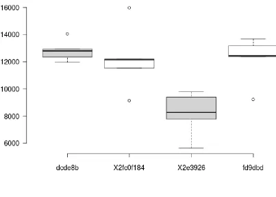
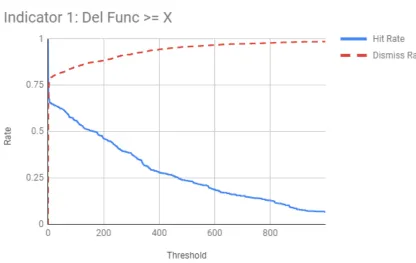
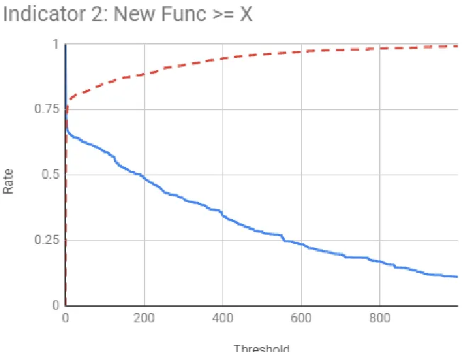
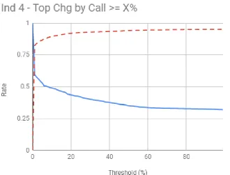
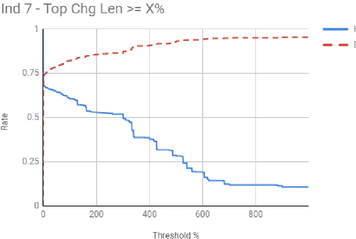
In order to answer the question of which indicators perform the best, we plotted the hit and
dismiss rate for each indicator for many different thresholds, on our full dataset of results.
We evaluated Indicators 1, 2, and 3 with threshold values from 0-1000, incrementing
by 1. We evaluated Indicators 4, 5, 7, and 8 with threshold values from 0-1 (0% - 100%)
incrementing by 0.01. As you can see, for each of these values the hit rate drops and the
dismiss rate spikes right at the first non-zero value. For your convenience, those first points
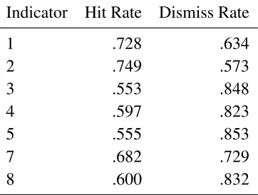
[image:28.612.220.401.528.665.2]are:
Table 6.2: Hit and dismiss rates for specific indicators
Indicator Hit Rate Dismiss Rate
1 .728 .634
2 .749 .573
3 .553 .848
4 .597 .823
5 .555 .853
7 .682 .729
Beyond this first point, the hit rate decreases and the dismiss rate increases, and tends
to level out at a certain threshold. If we define the best values for the indicators as the
values that give the highest hit rate while still actually dismissing some results, then the
threshold of 1 or 1% appears to be the best threshold for each of these values individually.
Furthermore, the best indicator, by that definition, would be indicator 2 - New Func ≥
X. Del Func is close, but it dismisses about 6% more at the cost of about 2% of the hits.
Indicator 8 dismisses about 23% more commits at that first threshold, but hits around 10%
fewer regressions.
Some other observations are that indicator 3 seems to have very little room between
hitting all the commits and hitting none of the commits, and that indicators 4, 5, 7, and 8
seem to quickly level out to a constant hit and dismiss rate, while for indicators 1 and 2 the
hit rate seems to decrease almost linearly as the threshold increases. Also, no matter what
threshold you pick, if you are using one indicator the best you can do for a hit rate with this
[image:29.612.97.513.422.685.2]data is 74.9%.
Figure 6.2: Indicator 2 - New Func≥X
Figure 6.4: Indicator 4 - Top Chg by Call≥X%
Figure 6.6: Indicator 7 - Top Chg Len≥X%
Chapter 7
Threats to Validity
In this chapter, we present factors that may impact the applicability of our observations in
real-life situations. We classify these factors into three categories [13].
Internal Validity. We report on the uncontrolled factors that interfere with causes and
effects, and may impact the experimental results.
Commits not necessarily sequential: The git project itself uses git as source control, and
employs a branching strategy with merges. If the project history branched and then merged,
when you view the history linearly you might have two commits next to each other which
technically were not developed sequentially when originally committed by the developer.
However, none of our metrics are dependent on that ordering. So, even if commit A is not
a direct parent to commit B in terms of how the development team wrote the code, our
system can still consider them as such because it makes no difference. In fact, if desired
we could jumble up the order of all the commits studied, and see if the system still works.
This would not be practical, because the amount of change between commits would likely
be dramatically higher, however for all our system knows the development team is just very
active and makes huge changes all the time.
Neither our study nor the original study consider accumulated change over time. Both
studies consider commits in pairs as they come in. If you have commits A, B, C, and D
pushed, in that order, Perphecy will evaluate the changes from A to B, then B to C, then C
to D. However, it may be more prudent to consider theaccumulatedchange over time, until
a hit occurs and we run our test again. In other words, assuming that the system predicts
after marking it as a dismiss, it would consider from A to C, then again after marking it
a dismiss, it would consider from A to D. With the way Perphecy works with thresholds,
if the predictor was, for example, ”Del Func ≥ 3”, and each commit involved deleting
one line, the first approach would not detect a performance hit, but the second approach
would, because the accumulated change would be marked as risky. In an extreme case
where a development team always limits commits to a single line of code, Perphecy would
likely not function properly. Considering accumulated change would fix this issue, and
may naturally decrease the need for periodic testing external to what Perphecy predicts.
Construct Validity.Herewith we report on certain challenges that validate whether the
findings of our study reflect real-world conditions.
Certain git code is platform dependent. We did not perform any testing on Windows
operating systems, so Windows specific code would not be executed during our dynamic
profiling, and thus any indicators depending on that profiling have no chance of activating
due to Windows specific changes.
The results of our experiments are influenced heavily by the definition of a performance
regression. We used the same definition as in the original paper, however this definition has
its limitations. For example, simply performing a t-test between two commits does not
consider the history of times. One could try performing a t-test between the samples of all
of the last X commits and the samples from the new commit. In a more realistic scenario,
running tests more than once would be unreasonable, so another approach could be keeping
a circular buffer of the last ten execution times and defining a regression as being a certain
number of standard deviations away from the mean. However, evaluating different methods
of defining performance regression is outside the scope of this work.
Using different computers for running performance tests: In order to execute the
per-formance tests for over 8000 commits in a timely manner, the task was parallelized across
multiple machines. This could become a threat because the results for the performance
and other random variables between machines. To mitigate this, identical digitalocean
(ci-tation?) VMs were used for all performance test results, which means CPU speed, RAM,
and so on were identical. Additionally, we ran each test 5 separate times, such that each
execution was at a different time of day on a different VM. This helps mitigate other
un-controllable random noise in the results of the testing.
External Validity. The prediction of performance regression was limited only to one
project. The generated predictor does not necessarily give the best results for other projects
[7]. This is due to the nature of changes performed by the developers, and so, for each set
of changes, there is eventually a need to refine the predictor. We mitigate this limitation
by simply re-executing our approach for the new system’s changes as input and update the
predictor.
Also, the diverse nature of commits may bias our results, we tired to address this
lim-itation by analyzing a large number of diverse commits written by multiple developers to
make the changes more representative. Similarly, not all projects utilize GitHub to track
and manage changes; and not all projects provide a performance testing set in the publicly
available source base. This may reduce the usability of our approach since is relies on
Chapter 8
Conclusion & Future Work
The goal of this work is to create a system which can accurately predict performance test
regressions. We have replicated the Perphecy paper on 8596 commits of the git project and
have found that the Perphecy approach does not perform as well as reported in the original
paper. The original paper found that for the same project on less commits, they were able to
correctly predict 85% of commits with regressions while correctly dismissing 83% of other
commits. In our study, we found that with our least aggressive cleaning of the training data
and our most realistic evaluation data set, a 76% hit rate with a 56% dismiss rate was more
realistic. We also identify and discuss a flaw in the original paper’s threshold selection
algorithm, and a larger dataset with further analysis on the individual indicators used in the
original study.
We plan to extend this study by adding additional indicators not considered in the
orig-inal paper. We plan to add five indicators based on 3 metrics - Flux, or the number of added
lines plus the number of deleted lines between two commits, Cyclomatic Complexity, and
Coupling between objects. Flux would provide a similar kind of indicator as number of
added functions or number of deleted functions, but it is based on lines rather than
func-tions. Some of the results we found that had only zero values for all the indicators would
have a non-zero value for flux. For cyclomatic complexity and coupling between objects,
we would look at the highest changed value between two commits, and also look at the
highest changed value that is also reached by the given benchmark. Though these are
typ-ically metrics used for correctness bugs, we wish to examine their impact on performance
This study can also be expanded to consider accumulated change, as discussed in the
Threats chapter. One last extension can be to experiment with different ways of using
the raw metric data other than determining static thresholds as is done in this study. For
instance, the values of the metrics could be fed directly into a neural network. Depending
on how the network is set up, this could lead to usage of conjunction between indicators as
Chapter 9
Acknowledgement
We would like to thank the members of the #git-devel IRC community for answering some
Bibliography
[1] Juan Pablo Sandoval Alcocer, Alexandre Bergel, and Marco Tulio Valente. Learning
from source code history to identify performance failures. InProceedings of the 7th
ACM/SPEC on International Conference on Performance Engineering, pages 37–48.
ACM, 2016.
[2] Gabriele Bavota, Abdallah Qusef, Rocco Oliveto, Andrea Lucia, and Dave
Bink-ley. Are test smells really harmful? an empirical study. Empirical Softw. Engg.,
20(4):1052–1094, August 2015.
[3] Shadi Ghaith, Miao Wang, Philip Perry, and John Murphy. Profile-based,
load-independent anomaly detection and analysis in performance regression testing of
soft-ware systems. InSoftware Maintenance and Reengineering (CSMR), 2013 17th
Eu-ropean Conference on, pages 379–383. IEEE, 2013.
[4] Peng Huang, Xiao Ma, Dongcai Shen, and Yuanyuan Zhou. Performance regression
testing target prioritization via performance risk analysis. InProceedings of the 36th
International Conference on Software Engineering, pages 60–71. ACM, 2014.
[5] Peng Huang, Xiao Ma, Dongcai Shen, and Yuanyuan Zhou. Performance regression
testing target prioritization via performance risk analysis. InICSE 2014 Proceedings
of the 36th International Conference on Software Engineering, pages 60–71. ACM,
2014.
[6] Qi Luo, Denys Poshyvanyk, and Mark Grechanik. Mining performance regression
inducing code changes in evolving software. In2016 IEEE/ACM 13th Working
[7] Nuthan Munaiah, Casey Klimkowsky, Shannon McRae, Adam Blaine, Samuel A.
Malachowsky, Cesar Perez, and Daniel E. Krutz. Darwin: A static analysis dataset
of malicious and benign android apps. InProceedings of the International Workshop
on App Market Analytics, WAMA 2016, pages 26–29, New York, NY, USA, 2016.
ACM.
[8] Thanh HD Nguyen, Bram Adams, Zhen Ming Jiang, Ahmed E Hassan, Mohamed
Nasser, and Parminder Flora. Automated detection of performance regressions using
statistical process control techniques. InProceedings of the 3rd ACM/SPEC
Interna-tional Conference on Performance Engineering, pages 299–310. ACM, 2012.
[9] Augusto Born de Oliveira, Sebastian Fischmeister, Amer Diwan, Matthias Hauswirth,
and Peter F. Sweeney. Perphecy: Performance regression test selection made simple
but effective. In2017 IEEE International Conference on Software Testing, Verification
and Validation (ICST), pages 103–113. IEEE, 2017.
[10] Fabio Palomba, Gabriele Bavota, Massimiliano Di Penta, Fausto Fasano, Rocco
Oliveto, and Andrea De Lucia. On the diffuseness and the impact on maintainability
of code smells: a large scale empirical investigation.Empirical Software Engineering,
Aug 2017.
[11] Michael Pradel, Markus Huggler, and Thomas R Gross. Performance regression
test-ing of concurrent classes. In Proceedings of the 2014 International Symposium on
Software Testing and Analysis, pages 13–25. ACM, 2014.
[12] Weiyi Shang, Ahmed E Hassan, Mohamed Nasser, and Parminder Flora. Automated
detection of performance regressions using regression models on clustered
perfor-mance counters. InProceedings of the 6th ACM/SPEC International Conference on
[13] Claes Wohlin, Per Runeson, Martin H¨ost, Magnus C Ohlsson, Bj¨orn Regnell, and
An-ders Wessl´en.Experimentation in software engineering. Springer Science & Business