Teaching mechatronics principles using laboratory classes

Teaching mechatronics principles using laboratory

classes

John Billingsley,

Faculty of Engineering and Surveying, University of Southern

Queensland,

Reg Dunlop,

Department of Mechanical Engineering, University of Canterbury.

The introductory module of a new course in mechatronics is based on

practical experiments in which the control is created entirely by the

student. Concepts of control system design in the presence of sharp

nonlinearities and of topology of the feedback structure are introduced and

illustrated with the example of an inverted pendulum, the culmination of

the first sequence of experiments. For a further experiment, a

three-wheeled variation on the mecanum mobile has been designed as the base

of a pendulum to be balanced in both directions.

Keywords:

Inverted pendulum, mecanum, feedback topology.

1. INTRODUCTION

An introductory module must give motivation to the students as well as starting to lay the foundations control theory relevant to mechatronics. The inverted pendulum experiment has the attraction of apparent difficulty, whereas a successful outcome can be achieved quite simply when the control task is viewed correctly. The task presents the essential problems of measurement and actuation, while a real-time control program can be created in terms of a few lines of code.

2. THE INVERTED PENDULUM

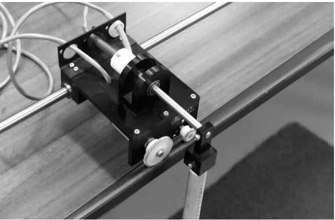
This well known experiment [1] provides exemplary problems of sensing and actuation. For the development of this particular sequence of experiments, using the opportunity of an Erskine Fellowship at the University of Canterbury, a much more sophisticated piece of existing apparatus was simplified to a suitable fundamental level.

Fig.1 Inverted pendulum apparatus

A 'trolley' is moved along a track by a motor. As seen in figure 1, a simple pinion on the end of a motor-gearbox runs on a rack. On the same rack runs a pinion driving a ten-turn potentiometer to provide a position signal. The students enter just seven lines of code in the controlling computer to create a function ADC() that will read an analogue channel.

As a 'half-way house' a position control experiment can be performed as one of a sequence of exercises. It demonstrates the need for a velocity signal, leading to an exercise in real-time signal processing to derive an approximate velocity from the position. The code to implement this is of the form

x = ADC(0)

v = kv * (x - xslow) xslow = xslow + v * dt

The students also become familiar with a simple H-bridge circuit and a software routine to convert a motor control value u into a mark-space output to the bridge.

With this, they can investigate the performance of a 'real' positioner, where the stiffness of the closed loop is of importance and can be tested by pushing against the trolley. A satisfactory result requires near-bang-bang control. It is found that suitable velocity feedback to avoid overshoot requires a gain many times the 'textbook' value [2]. They perceive the crisp performance that can be achieved and that will certainly be demanded by an industrial client.

Measurement of the tilt angle of the pendulum is performed with a simple Hall-effect sensor and a small magnet. When the rod is vertical, the field cuts the sensor 'edge on'. As the rod tilts there is a component of the magnetic field normal to the sensor and a voltage output is obtained.

Software to read the tilt and estimate its derivative is almost identical to the code used for position and velocity. Closing the feedback loop to achieve good performance presents a few more problems, however.

3. FEEDBACK TOPOLOGY

When a system and its controller are both linear, the state equations can be arranged in numerous ways to represent the same simple arrangement whereby each input is calculated from a linear combination of state variables. The characteristic equation is simply determined and the control design usually hinges on selection of parameter values to place the poles in desirable locations [3, 4].

Few if any of the systems encountered by the mechatronic engineer are linear. For example any motor has a drive that limits when the full supply voltage is applied. To over design the system so that full drive is seldom applied is not economic. When performance and safety are paramount, the limitations and nonlinearities play a dominant part in system design. Even more important for complex systems can be the consideration of zero placement. The algebra reflects the answer to "What is fed back to where?"

By way of an example, consider the pitch control channel of an aircraft. There are two significant inputs, the elevator and the throttle. The variables that must be controlled by them are the airspeed and the height. A simplistic approach to the topology of the feedback structure would be to use the velocity error to determine the throttle setting and the height error to dominate the elevator.

Given a low-speed stall warning, however, the first action of an experienced pilot is to 'push the stick forward'. Speed fluctuations may more readily and safely be controlled with the elevator, while opening the throttle can be seen to apply more power to enable the aircraft to climb at constant speed.

We see the decomposition of the control task into sub-loops, with a structure that can be viewed as a question of topology.

3.1 The bicycle and the pendulum

proportional acceleration. The bicycle's wheel displacement acceleration is proportional to the handlebar angle (to a fair approximation) while the trolley's acceleration is proportional to the motor drive. In both cases there is a hard input constraint, when full voltage is applied to the motor or when the handlebar hits the rider's knee.

The lateral acceleration of the rider is proportional to the bicycle's angle of 'lean' while the acceleration of the top of the pendulum is proportional to its tilt. From these, the acceleration of the wheel and trolley must be subtracted, respectively, to yield the accelerations of lean and tilt angles.

For the purpose of teaching the principles we make a number of simplifying assumptions. We assume that the no-load speed of the trolley motor is high, so that for now the 'back emf' damping can be neglected. We assume that both rider and pendulum behave as a point mass and that the effect of the pendulum on trolley acceleration can be neglected.

If we define the handlebar and the motor inputs both to be u and trolley and wheel displacements to be x, we have:

d2x/dt2 = b1 u for the bicycle and

d2x/dt2 = p1 u for the pendulum, while

d2lean/dt2 = (g lean - b1 u)/h and

d2tilt/dt2 = (g tilt - p1 u)/h

where h is the length of the pendulum or the height of the rider above the ground. p1 is the full-drive acceleration of the trolley motor, while b1 is proportional to the square of the bicycle velocity divided by its wheelbase. In both cases we may take u to be limited in magnitude to unity.

Whereas the inverted pendulum is regarded as a challenging control task, the bicycle can be mastered at a very early age!

3.2 Analysis of the pendulum

A simple linear feedback scheme can see u expressed in terms of the four state variables x, dx/dt, tilt and dtilt/dt as

u = (a x + b dx/dt + c tilt + d dtilt/dt)/p1

and the characteristic equation is then obtained as

s4 + (d/h - b)s3 + (c/h - g/h - a)s2 +(b g/h)s + a g/h = 0

A glance at the coefficients will reveal that in requiring them all to be positive for stability, the position and velocity feedback coefficients must also be positive. This might come as a surprise to at least one major vendor of laboratory experiments.

controlled position loop for the trolley, we are already committed to a large amount of negative position feedback that must be countered in an external loop.

If instead we take our lead from the cyclist, we must concentrate first on the 'tilt' or 'lean' loop that presents a threat of falling over. A positive value of c will cause the trolley to drive to the right in response to a tilt to the right - the trolley will run underneath the pendulum bob. A positive value of d will add damping to this 'power assisted steering' effect; holding the top of the pendulum will cause the trolley to power to a position that keeps the stick vertical.

Provided the value of c is substantially greater than g, this inner loop will be stable even when the pendulum top is briefly released. Quickly, however, the trolley will drift to one end or the other and a violent reaction will result. It is necessary to control the trolley’s position.

Once again the experience of the cyclist can be drawn upon to give an intuitive solution. To turn, a cyclist demands a lean angle in the direction of the desired turn. If the trolley is displaced to the right and we wish it to move to the left, we must demand that the pendulum lean to the left and the tilt loop will do the rest. In order to cause the pendulum to lean to the left the trolley must first move further to the right – and once again we see the application of positive position feedback.

It is a relatively straightforward matter for the students to hold the top of the pendulum and move it from side to side while the trolley tracks it, noticing the ‘virtual pivot’ above the pendulum top defined by the position feedback gain. They adjust this gain in their software to give a pivot height of about two metres, add a modicum of positive velocity feedback and the tuning task is done. All that remains is the algebraic analysis to see why it works and an investigation of the merits of limiting the tilt angle demand.

4. AN EXTRA DIMENSION

For the second stage, the linear track is replaced by a two-dimensional mecanum-style trolley, to be driven to balance the pendulum in two dimensions. This is shown at a prototype stage in figure 2.

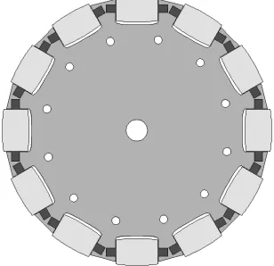
As can be seen in the drawing of figure 3, the wheels have ‘tyres’ of miniature wheels or rollers. In the ‘true mecanum’ [5], these are skewed to overlap so that rolling is smooth. Instead, we accept the ‘lumpiness’ as contact passes from one roller to the next in exchange for a simpler kinematic equation. If the three rim velocities are A, B and C, then azimuth rotation of the platform is proportional to A + B + C, while motion in two orthogonal directions is defined by modes in which

A = - B, C = 0 for one mode and A = B = -2 * C for the other.

Fig. 2. A Three-wheeled trolley

Fig. 3. Arrangement of rollers around the rim of each wheel

5. CONCLUSIONS

those regarded as its components. By stripping the task to bare unadorned essentials, the fundamental concepts can be grasped in a way that gives confidence in the associated mathematical analysis.

The embellishment added by the two-dimensionally moving base will probably not add much to the theory already grasped by the students, but it will stick in their minds as a spectacular demonstration.

Acknowledgment

This collaboration was made possible through an Erskine Fellowship at the University of Canterbury, Christchurch, New Zealand.

References

1. Shao, J. Inverted Pendulum Systems for Mechatronics Education. Proc. 2nd Int. Conf. on Mechatronics and Machine Vision in Practice, pp. 320-325, Hong Kong, September 1995

2. J Billingsley, On the design of position control systems, Proc IEE Part D, vol 138, no 4, July 1991, pp 331-336.

3. Carnegie Mellon University and University of Michigan ‘8/11/97 CJC’, Control tutorials for Matlab,

http://www.engin.umich.edu/group/ctm/examples/pend/invpen.html 4. University of Newcastle notes on control system design http://csd.newcastle.edu.au/control/simulations/pend_sim.html