Process capability for a complete electronic product assembly

Rochester Institute of Technology

RIT Scholar Works

Theses Thesis/Dissertation Collections

6-2016

Process capability for a complete electronic product

assembly

Flavia Carvalho Resende [email protected]

Follow this and additional works at:http://scholarworks.rit.edu/theses

This Thesis is brought to you for free and open access by the Thesis/Dissertation Collections at RIT Scholar Works. It has been accepted for inclusion in Theses by an authorized administrator of RIT Scholar Works. For more information, please [email protected].

Recommended Citation

Process capability for a complete electronic product

assembly

by

Flávia Carvalho Resende

Thesis submitted in partial fulfillment of the requirements for the

Degree of Master of Science in Manufacturing and Mechanical System

Integration

Rochester Institute of Technology

College of Applied Science & Technology

Department of Manufacturing and Mechanical System

Integration

Rochester Institute of Technology

College of Applied Science & Technology

Master of Science in Manufacturing and Mechanical System

Integration

Thesis Approval Form

Student Name: Flávia Carvalho Resende

Thesis Title:

Process capability for a complete electronic product

assembly

Thesis Committee

Name

Signature

Date

Dr. Robert Parody

Chair

Dr. S. Manian Ramkumar

Committee member

Dr. James Lee

Abstract

There are many studies about the process capability indices which are used to study if a

process can meet specification. Unfortunately, there are few studies about the product capability.

So, the main aim of this thesis is to present an alternative to determine the product capability. It

is important to determine if when the quality characteristics of a product are assembled the final

product will still meet the specification. This study proposes an approach to determine the

product capability using the 𝐶_𝑝𝑚 to analyze the capability of the quality characteristic. Also, this

thesis proposes the use of weight to determine the influence of the quality characteristic in the

final quality of the product. This study was divided in four steps, the first one the definition of

the product and quality characteristics that will be used. The second one is the simulation study

where the estimators used to determine the process capability indices are defined. The third one

is the characteristic study which presents the CPI and the yield for the characteristics analyze.

Acknowledgments

I would like to present my gratitude to who, directly and indirectly, helped to conclude

this thesis.

Professor Dr. Robert Parody, who accepted to be my adviser and guided me during all the

process to develop this project.

Professor Dr. Manian Ramkumar, who help me to better understand the project and open

my mind about the paths that this project could take.

My mother, who always supported me and even away, is present in my day, taking care

of me and being an example to me.

My brothers, Samuel and Thyago, who are always there for me.

My friends from Brazil, who even away are present in my day.

My friends from here, especially, Marcos, Celline, Danial, Mariah, Aaron and

Alessandra, who make easier these two years away from my hometown.

And finally, I would like to thank CAPES/CNPq for funding my master program under

the Brazilian Scientific Mobility Program (Ciência sem Fronteiras), process number

I

Table of Contents

1. Introduction ... 1

2. Related Work ... 3

2.1. Process Capability ... 3

2.1.1. Process Capability Index 𝑪𝒑 ... 3

2.1.2. Process Capability Index 𝑪𝒑𝒌 ... 5

2.1.3. Process Capability Index 𝑪𝒑𝒎 ... 5

2.2. Process Capability for entire product ... 6

2.3. Sensitivity Analysis ... 10

2.4. Process capability in the electronic industry ... 11

3. Methodology ... 13

3.1. Define the product ... 13

3.2. Simulation Study ... 13

3.2.1. Sample Size Analysis ... 14

3.3. Characteristic Study ... 14

3.4. Product Study ... 16

3.4.1. Determining the weight 𝒘𝒊... 18

3.4.2. How to analyze the product to determine the product capability ... 18

3.4.3. Process capability using the PCIs ... 19

3.4.4. Process capability using the yield ... 21

3.4.4.1. Process capability for nom-normal samples ... 22

4. Results ... 25

4.1. Define the product ... 25

4.2. Simulation Study ... 25

4.3. Characteristic Study ... 26

4.4. Product Study ... 26

4.4.1. Determining the weight 𝒘𝒊... 26

4.4.2. Product capability using the PCIs ... 32

II

5. Discussion... 38

5.1. Simulation Analyses ... 38

5.2. Quality Characteristics Analyses ... 38

5.3. Product Capability Analyses ... 43

6. Conclusion ... 45

7. Reference ... 47

Appendix A: Yield to Process Capability Conversion (𝑪𝒑𝒌) ... 50

Appendix B: Yield values for different 𝑪𝒑𝒎 ... 51

Appendix C: Simulation Study ... 53

Appendix D: Data Assumption Test ... 54

III

List of Figures

Figure 1 Distribution for five different samples (Montgomery, 2009) ... 4

Figure 2 MPPAC with capability zones ... 9

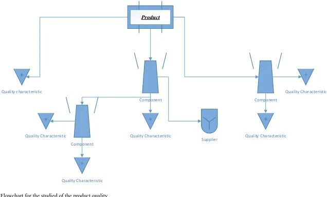
Figure 3 Flowchart for the studied of the product quality ... 20

Figure 4 Flowchart methodology ... 24

Figure 5 H-type chip resistor (Ouyang et al., 2013) ... 27

IV

List of Tables

Table 1 The Cpm values and respective yield (Chen and Huang, 2007) ... 17

Table 2 Probability Distributions and their respective yield ... 23

Table 3 : Specification of the H-type chip resistor(unit: mm) (Ouyang et al., 2013) ... 28

Table 4: Mean and variance for the quality characteristic. ... 29

Table 5: PCIs for the quality characteristics ... 30

Table 6 Yield for the quality characteristics ... 31

Table 7 Process capability for the components using the PCIs ... 33

Table 8 Process capability for the components using the PCIs (without weight) ... 34

Table 9 Process capability for the components using the yield ... 35

Table 10 Process capability for the components using the yield (without weight) ... 37

Table 11 Comparison between the real data and the simulation data ... 40

Table 12 Quality characteristics summary results ... 41

V

Table of Abbreviations

PCI Process Capability Index

LSL Lower Specification Limit

USL Upper Specification Limit

1

1. Introduction

Quality is the new wave trend for companies nowadays and for good reason. Every

company wants to reduce their costs and increase customer satisfaction. The best way to do this

is by increasing the quality management of their products. By doing this, the number of

nonconformities and the time spent in inspection will decrease alongside with the increase in

reliability of the product and customer satisfaction. Usually, the increase of quality will result in

the increase of total cost, so it is extremely important to balance this quality improvement with

the final cost of the product.

To achieve this balance, it is necessary to determine the deficiencies of the process, the

best yield of the components, and to identify the improvements that will have more of an impact

on the quality of the process. Unfortunately, in general, the resources available for improvements

are limited. It is difficult to determine the deficiencies of the process because a product is made

of different components with different standard quality characteristics (Ouyang, Hsu, & Yang,

2013). Also, a consequence of this process complexity is that it is hard to determine what

improvements will have more of an impact on the final product.

In the electronic industry, these difficulties are even worse. The tolerance design of the

components is tight, so the stability and reliability of the components will have a high impact on

the quality of the product. Even small deviation can cause unpredictable results to the system

(Zhai, Zhou, Ye, & Hu, 2013). Besides this, the output of some components will directly impact

the output of others, so it is extremity important to analyze all of the connections between the

parts and determine which components are more crucial for the whole product.

Due to all of these difficulties, there are many studies about the improvement of quality,

2

three parameters that have been widely used to measure the ability of the process to meet

specification, they are the process yield, process expected loss, and the process capability indices

(PCIs) (Chen, Huang, & Li, 2001). The process yield is the percentage of products units that

pass the inspection, the process expected quality loos is the cost related with poor quality, and

the PCIs are indices used to determine if a process if capable to meet the specifications. The

higher the PCIs and process yield, the lower the cost due to poor quality.

There are many studies about PCIs and how they can be used to determine if a product

meets the specifications. In this research, several methodologies to determine the process

capability of an entire product is presented. Given this background, the best approach to analyze

the process capability of electronical products is chosen. The Monte Carlo simulation will be

utilized to generate the data that will be used to determine the PCIs values. The report will also

3

2. Related Work

2.1.Process Capability

The process capability indices are used to determine if a process is capable of producing

products within a specification limit. It is important to remember that the use of the PCIs is

recommended just for the process in statistical control, in other words, in any process where

special causes of defects were identified and removed (Shewhart, 1939). In general, the PCI will

compare the natural variability of the process and can be defined as

𝑃𝐶𝐼 =𝐴𝑙𝑎𝑤𝑎𝑏𝑙𝑒 𝑝𝑟𝑜𝑐𝑒𝑠𝑠 𝑠𝑝𝑟𝑒𝑎𝑑

𝐴𝑐𝑡𝑢𝑎𝑙 𝑝𝑟𝑜𝑐𝑒𝑠𝑠 𝑠𝑝𝑟𝑒𝑎𝑑

(2.1)

In the last twenty years, several process capability indices were proposed. The first

generation process capability index is based on the idea that if the process is within specification

limits, the quality of the product will be good (Kureková, 2001). There are two first generation

PCIs, the 𝐶_𝑝 and the 𝐶_𝑝𝑘.

2.1.1. Process Capability Index 𝑪_𝒑

The 𝐶_𝑝 was proposed by Juran (1974) and is defined as

𝐶_𝑝 = 𝑈𝑆𝐿 − 𝐿𝑆𝐿

6 ∗ 𝜎 =

𝑑 3 ∗ 𝜎

(2.2)

Where the USL and LSL are the upper and the lower specification limit respectively, the

σ in the process standard deviation and the 𝑑 is the half specification.

The 𝐶_𝑝 measures the variability of the process relative to the specification limits, so the

bigger its value, the smaller the variability will be. This index doesn’t take into account the

deviation of the process mean from the target value and how the data is spread within the

4

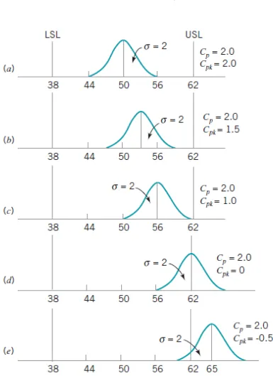
when the process has high variability and out of target. Figure 1 shows five different process

samples that present a similar 𝐶𝑝 value:

5

Looking at Figure 1, the five samples present similar standard deviations, so the 𝐶_𝑝

values are similar. Observing this result, it is possible to assume that all the processes are capable

but this assumption is wrong. The processes present data out of the specification limits and the

mean for the processes b, c, d and e are off target. Only process “a” is capable.

2.1.2. Process Capability Index 𝑪_𝒑𝒌

To overcome this problem, Kane (1986) proposed the 𝐶_𝑝𝑘, this index takes into

consideration the deviation of the process mean from the target value. The 𝐶𝑝𝑘is defined as

𝐶_𝑝𝑘 = 𝑚𝑖𝑛𝑖𝑚𝑢𝑚 {𝐶_𝑝𝑢 , 𝐶_𝑝𝑙}= 𝑚𝑖𝑛𝑖𝑚𝑢𝑚 {𝑈𝑆𝐿−µ

3𝜎 , µ−𝐿𝑆𝐿

3𝜎 }

(2.3)

Where µ is the process mean.

Looking at figure 1 the distribution of the data affects the 𝐶_𝑝𝑘 and also, that of the 𝐶_𝑝𝑘 is

equal or smaller than the 𝐶𝑝. These values will be equal when the process is on target and when

the data mean is equal to the target process.

The 𝐶𝑝 and 𝐶𝑝𝑘 are independent of the target value, so the use of these indices are

recommended for cases where the reduction of the variability and process yield are important

(C.-W. Wu, Pearn, & Kotz, 2009). When the target differs from the mean between the upper and

lower specifications, these process capabilities indices will lead to the wrong acceptance of the

process. In contrary, these indices don’t analyze the cost related with the departure from the

target.

2.1.3. Process Capability Index 𝑪𝒑𝒎

To overcome these limitations, the second generation process capability index (𝐶_𝑝𝑚) was

proposed. Being within the specification limits alone will not be enough to ensure that the

product has high quality, it is also necessary to analyze how the values studied are spread within

6

The 𝐶_𝑝𝑚was proposed by (Chan et al., 1988) and (Hsiang & Taguchi, 1985)

independently and it is defined as

𝐶_𝑝𝑚 = 𝑈𝑆𝐿 − 𝐿𝑆𝐿

6(𝜎2 _{+ (µ − 𝑇)}2₎1/2

(2.4)

Where T is the target value of the process. Looking at this equation, it is possible to

notice that the minimum value of 𝐶_𝑝𝑚is 0 and that the maximum value will occur when µ − 𝑇 =

0 and this value is equal to 𝐶𝑝, so

0 ≤ 𝐶_𝑝𝑚 ≤ 𝑈𝑆𝐿 − 𝐿𝑆𝐿

6 ∗ 𝜎 = 𝐶𝑝

(2.5)

To apply these PCIs to analyze a process, the sample used in the study must follow a

normal distribution in order to calculate the PCIs necessary to use as estimators to replace µ

(process mean) and 𝜎 (process standard deviation). Instead of using µ and 𝜎, the sample mean

(𝑋̅) and the sample variance (S) will be used. They are defined as

𝑋̅ = ∑𝑥𝑖 𝑛

𝑛

𝑖=1

(2.6)

S = √∑(𝑥𝑖−𝑥̅)

2

𝑛 − 1

𝑛

𝑖=1

(2.7)

For a sample that follows the normal distribution these estimators will be reliable, but for

a different distribution they are not dependable. Other more appropriate and complex PCIs must

be used (Pearn & Chen, 1997).

2.2.Process Capability for entire product

In relation to the information presented in the previous section, the process capability

7

single product’s characteristic. However, it is necessary to determine if when all these processes

are put together, if the final product will also be able to meet the specifications required.

To determine the process capability of a final product some approaches were proposed.

The first approach to calculate the process capability for an entire product was presented by

Bothe (1992). Overall, this method uses the characteristic yield to determine the process

capability of the product. Firstly, it is necessary to determine the yield of each characteristic and

in order to determine this value it is necessary to calculate the 𝑍_𝑈𝑆𝐿and 𝑍_𝐿𝑆𝐿, that are defined as

𝑍𝑈𝑆𝐿 =

𝑈𝑆𝐿 − µ 𝜎

(2.8)

𝑍𝐿𝑆𝐿 =

µ − 𝐿𝑆𝐿 𝜎

(2.9)

Using the 𝑍𝑈𝑆𝐿 and the Z-table it is possible to determine the probability of the product

be below the upper specification limit (Prob. Bad Below) and the probability of the product to be

above the upper specification limit (Prob. Bad Above). The yield of the characteristic with

bilateral specification is equal to

𝑌𝑖𝑒𝑙𝑑𝑛 = 𝑃𝑟𝑜𝑏. 𝐺𝑜𝑜𝑑 = 1 − (Prob. Bad Below + Prob. Bad Above) (2.10)

For unilateral specification, the yield will be determined as

𝑌𝑖𝑒𝑙𝑑_𝑛 = 𝑃𝑟𝑜𝑏. 𝐺𝑜𝑜𝑑 = 1 − (Prob. Bad Below or Prob. Bad Above) (2.11)

The yield of the product will be equal to the product of the yield of all characteristics, as

shown below

𝑃𝑟𝑜𝑑𝑢𝑐𝑡 𝑌𝑖𝑒𝑙𝑑 = ∏ 𝑌𝑖𝑒𝑙𝑑𝑛

𝑛

𝑖=1

(2.12)

Using this information is possible to determine the 𝐶_𝑝𝑘 of the product using the

8

𝐶_𝑝𝑘 = 𝑍𝑆𝑐𝑜𝑟𝑒 3

(2.13)

Where the 𝑍_{𝑆𝑐𝑜𝑟𝑒} is determined using Z-table and the probability (𝑝_𝑏𝑎𝑑) that the product

will not meet specification, this value is defined as

𝑝_𝑏𝑎𝑑 =1 − 𝑝𝑟𝑜𝑑𝑢𝑐𝑡 𝑦𝑖𝑒𝑙𝑑

2

(2.14)

For each 𝐶_𝑝𝑘 value there is a respective yield value for the product. For example, for

𝐶𝑝 = 1, the yield of the process is equal to 93.30%. Appendix A presents example 𝐶𝑝𝑘 and its

respective yield.

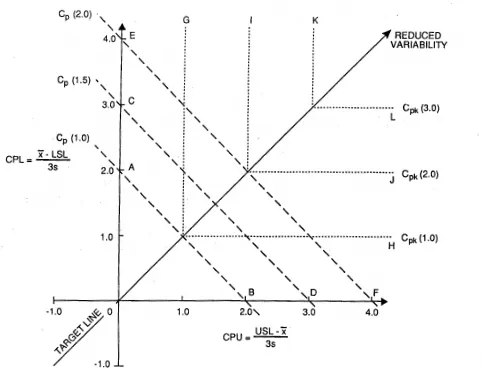
Another method used to analyze the product capability was proposed by Singhal (1990).

He presented a visual tool, the Multiprocess Performance Analysis Chart (MPPAC), that presents

how the processes behaves in a multi process environment. The chart shows the 𝐶_𝑝, 𝐶_𝑝𝑘, the

departure of the process mean from the target, and the variability of the process. One of the

limitations of this chart is that it does not present where the process capability must be to ensure

the quality of the product, so it is not possible to analyze the performance of the process.

To overcome this problem, Singhal (1992) proposed an improvement to the chart. He

added capability zones to it . Figure 1 presents this chart.

This is a very useful visual tool to analyze different processes, but the chart presents

some limitations it that it cannot be used to determine the final product quality. Other charts

(Chen et al., 2001; Ouyang et al., 2013) were proposed to analyze multi-processes, but they were

9

10

Nowadays, there is an approach that studies the product capability and has been widely

used (Chen et al., 2001; C. C. Wu, Kuo, & Chen, 2004; Yu, Sheu, & Chen, 2007). Knowing that

𝑝 = ∏ 𝑝𝑖

𝑛

𝑖=1

(2.15)

This method assumes that for a desired 𝑝, the product yield, the characteristic yield must

be at least 𝑝_𝑖 = 𝑝1/𝑛. To apply this equation, the characteristics must to be independent. This

information can be added to the charts presented to help to determine the capability zones. This

is a quick way to determine the product capability but this method will result in some loss.

When a minimum value for the yield of the product is fixed, all the characteristics need to

meet this requirement. In many cases, some parts of the product don’t need to present high

quality as the final product and occasionally the part that is critical for the product and this

minimum value is not enough to ensure the quality of the final product. The best approach is to

look each part individually first and determine the specifications and level of quality of each one

looking how it will impact in the final product.

2.3.Sensitivity Analysis

With the data presented, it is possible that it may still be missing some important

information to determine the process capability of a product. These approaches don’t take into

consideration the level of impact of quality of different characteristic in the final product. When

the process capability of the product is calculated, it is necessary to take in consideration the

weight of the unit (Mu, He, Chang, & Ma, 2009).

Yu, Sheu & Chen (2007) presented one approach to add the influence of importance of

the characteristic in the calculation of the process capability for the product. Their proposal

11

𝑃𝐶𝐼𝑐𝑚 = [∏(𝑃𝐶𝐼_𝑖)𝑤𝑖

𝑛

𝑖=1

]

1 ∑𝑛𝑖=1𝑤𝑖

(2.16)

Where 𝑤_𝑖 is an integer number between 1 and 5. The most important characteristic will

have 𝑤_𝑖 = 5 and the less important 𝑤_𝑖 = 1.

Another alternative was proposed by Mu at el (2009). In his approach, firstly, the weight

is multiplied by the PCI and then all the PCIs are summed. The equation proposed by him is

presented bellow

𝑃𝐶𝐼𝑇2 = ∑ 𝑤𝑖

𝑛

𝑖=1

∗ 𝑃𝐶𝐼𝑖

(2.17)

Where 𝑤𝑖 is a number between 0 and 1.

To determine the value of the weight is important to look the type of process that will be

analyzed. For example, for a medical process, the characteristics must to be studied take into

account the risk that poor quality will have to the patient. The scale used to the weight must be

aligned to the safety of the patient. For a mechanical process, the weight must to be decide

following the characteristics that will have a bigger impact in the functionality of the product.

2.4.Process capability in the electronic industry

The electronic products are different than others types of products, due to tighter

tolerance and specification limits, so the process yield sensitivity will have a bigger impact in the

quality of the product (Huang & Kong, 2010). It is extremely important to determine the best

tolerance requirements and specification limits. Spence (1984) presented a parameter space,

which is a chart that uses as a input the output of different characteristics and relate these

information. He presents an idea of cost and quality balance, so the parameter space will not be

12

It is important to do a sensitivity analysis to determine what parameters will be

13

3. Methodology

This research aims to present an approach to determine the process capability of

electronic products. This research was divided into 4 phases: define the product, simulation

study, quality characteristic study and product study.

3.1.Define the product

To start this analysis, it is necessary to determine the product that will be studied and

what quality requirements are. Knowing the product, the next step is to determine the quality

characteristics that will be used to determine the quality of the final product.

The quality characteristic is a quantitative characteristic of a component that has impact

on the quality of the final product. This characteristic can be measured and its data is used to

determine if the characteristic does or does not meet the specifications.

For each quality characteristic, it is necessary to determine the specification limits, mean,

standard deviation, target, and quality requirements. The data acquired will be used to determine

the yield and the process capability indices.

3.2.Simulation Study

To calculate the yield and the process capability indices of the characteristics, it is

necessary to calculate their estimator, that is the sample mean (𝑋̅) and the sample variance (𝑆2).

To determine these values, a sample of the process data is required. This sample can be obtained

in two ways: using real data of the manufacturing process or using a simulation.

To obtain the data using the first option is not easy, it is necessary to find a company

record of the data as well as permission to use such information, so the second option was used

14

random data using the sample mean and standard deviation. To run the Monte Carlo simulation,

the first step to determine the sample size.

3.2.1. Sample Size Analysis

It is necessary to determine the sample size for each one of the characteristics. To

determine this number, the following equation will be used

𝑛 = [100 ∗ 𝑧 ∗ 𝑆

𝐸 ∗ 𝑥̅ ]

2 _(3.1)

Where z is the z-score related to the confidence interval required for the data, E is the

error percentage acceptable for the mean. The equation presents three unknown variables: n, S

and 𝑥̅. For this case, 𝑆 and 𝑥̅ can be replaced by the historical data, σ and µ respectively (Driels

& Shin, 2004). How the characteristics differ in mean and variance, the sample size will be

different as well. But, how the same product is being analyze, the sample size will be equal to the

sample size of the characteristic that has the bigger value.

This research uses electronic products as the subject. The variance and tolerance for this

kind of product is tight, so any variance can result in impact of the quality of the product. The

confidence interval must to be high and the error must to be low.

Using the sample size, standard deviation, and mean it was possible to create random data

for all of the characteristics. It is important to remember that the data must be in statistical

control and must follow the normal distribution.

3.3.Characteristic Study

Using the estimators calculated in the section Simulation Study, it will be possible to

determine the yield of the characteristic and the process capability index. In this project, the 𝐶𝑝,

𝐶_𝑝𝑘 and 𝐶_𝑝𝑚 were calculated and compared. To determine the value of these indices, the

15

𝐶𝑝𝑖=

𝑈𝑆𝐿 − 𝐿𝑆𝐿

6 ∗ 𝑆 =

𝑑 3 ∗ 𝜎

(3.2)

𝐶_𝑝𝑘𝑖 = 𝑚𝑖𝑛𝑖𝑚𝑢𝑚 {𝐶_𝑝𝑢 , 𝐶_𝑝𝑙}= 𝑚𝑖𝑛𝑖𝑚𝑢𝑚 {𝑈𝑆𝐿−𝑥̅

3∗𝑆 , 𝑥̅−𝐿𝑆𝐿

3∗𝑆 }

(3.3)

𝐶𝑝𝑚𝑖 =

𝑈𝑆𝐿 − 𝐿𝑆𝐿 6(𝑆2_{+ (𝑥̅ − 𝑇)}2₎1/2

(3.4)

Where 𝑖 is a number between 1 and n.

It was also used to calculate the yield of the product using the 𝐶_𝑝𝑘 and 𝐶_𝑝𝑚. The yield

using the 𝐶𝑝𝑘 is calculated following the equation x

𝑝𝑖 = %𝑌𝑖𝑒𝑙𝑑 = ϕ(3 ∗ 𝑍_𝑚𝑖𝑛) (3.5)

The Appendix A presents a table with the yield value for respective 𝐶_𝑝𝑘.

To determine the yield using the 𝐶𝑝𝑚, it is necessary to use the equation proposed by

Chen and Huand (2007). The relationship is presented below

𝑝𝑖 = %𝑌𝑖𝑒𝑙𝑑 = ϕ (1 + √1/(3 ∗ 𝑐)

2_{− (S/𝑑)}2

𝑆/𝑑 ) + ϕ (

1 − √1/(3 ∗ 𝑐)2_{− (S/𝑑)}2

𝑆/𝑑 )-1

(3.6)

Where 𝐶𝑝𝑚𝑖 = 𝑐, 𝑑 = (𝑈𝑆𝐿 − 𝐿𝑆𝐿)/2.

Knowing that

0 ≤ 𝐶_𝑝𝑚 ≤𝑈𝑆𝐿 − 𝐿𝑆𝐿

6 ∗ 𝜎 =

𝑑 3 ∗ 𝜎

(3.7)

We conclude that 𝜎/𝑑 is between zero and 1/3𝑐. This relationship can be approximated

to 𝜎 𝑑 = ℎ 30∗𝑐 (3.8)

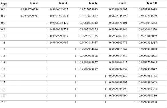
Where h is a integer number between 1 and 10. Using this relationship, Chen and Huang

16

presents these result. Appendix b presents the table with the yield values for 𝐶_𝑝𝑚 varying

between 0 and 1 with 0.01 as increments and h varying between 1 and 10.

For the unilateral specification, the 𝐶𝑝𝑙 and the 𝐶𝑝𝑢 will be used as process capability

indices. In this case, for the characteristics with lower specification limits, the yield and the 𝐶_𝑝𝑙

will be calculated as

𝐶𝑝𝑙𝑖 = (1/3)𝜙−1∗ (𝑝𝑙)

𝑝𝑙 = %𝑌𝑖𝑒𝑙𝑑 = 𝑃(𝑥 > 𝐿𝑆𝐿) = 𝜙(3𝐶𝑝𝑙𝑖)

For the characteristics with upper specification limits, the yield and the 𝐶_𝑝𝑢 will be

calculated as

𝐶𝑝𝑢𝑖 = (1/3)𝜙−1∗ (𝑝𝑢)

𝑝𝑢 = %𝑌𝑖𝑒𝑙𝑑 = 𝑃(𝑥 < 𝑈𝑆𝐿) = 𝜙(3𝐶_𝑝𝑢𝑖)

3.4.Product Study

The last phase of this study is to determine the process capability of the product. To

determine the product process capability, two approaches were used: using the process capability

indices and process yield. Aside from the PCIs and the yield, it is necessary to know the

influence of each characteristic in the quality of the final product. This influence is numeral

17

Table 1 The C_pm values and respective yield (Chen and Huang, 2007)

𝑪_𝒑𝒎 𝐡 = 𝟐 𝐡 = 𝟒 𝐡 = 𝟔 𝐡 = 𝟖 𝐡 = 𝟏𝟎

0.6 0.9999794334 0.9864026657 0.9522023043 0.9318429007 0.9281393618

0.7 0.9999999893 0.9984553624 0.9848691887 0.9692345598 0.9642711589

0.8 1 0.9998958420 0.9961695712 0.9876871101 0.9836049282

0.9 1 0.9999958773 0.9992290125 0.9956490149 0.9930660524

1.0 1 0.9999999049 0.9998771335 0.9986467043 0.9973002039

1.1 1 0.9999999987 0.9999845457 0.9996303775 0.9990331517

1.2 1 1 0.9999984694 0.9999115067 0.9996817828

1.3 1 1 0.9999998808 0.9999814540 0.9999038073

1.4 1 1 0.9999999927 0.9999966013 0.9999733085

1.5 1 1 0.9999999997 0.9999994559 0.9999932047

1.6 1 1 1 0.9999999239 0.9999984133

1.7 1 1 1 0.9999999907 0.9999996603

1.8 1 1 1 0.9999999990 0.9999999334

1.9 1 1 1 0.9999999999 0.9999999880

18

3.4.1. Determining the weight (𝒘_𝒊)

The weight was calculated comparing the influence of the quality characteristic in the

final quality of the product. The higher value is given to the most important characteristic and the

weight of the other characteristics will be determined based on the most important one. There are

many ways to determine the weights; to standardize it, each characteristic was assigned a value

𝑘_𝑖 between 1 to 10, where 10 is the most important and 1 is the least important quality

characteristic.

Using these values, it is possible to determine 𝑤_𝑖 for any approach. For example, for the

approach presented by Yu et al. (2007), 𝑤_𝑖 is a number between 1 and 5, so it will be equal to

𝑤_𝑖 = 𝑘_𝑖/2 (3.9)

For the approach presented by Mu at el (2009), 𝑤𝑖 is a number between 0 and 1, so it will

be equal to

𝑤𝑖 =

𝑘_𝑖 ∑𝑛𝑖=1𝑘𝑖

(3.10)

3.4.2. How to analyze the product to determine the product capability

To manufacturing a product, many parts must to be assembled together. A company can

manufacture all the components need or can get it from outside suppliers. When we try to

determine the quality of the product all this parts used to manufacture the product must to be

studied such as the quality of the characteristics, the components quality and the quality of the

parts provided by the suppliers.

The quality characteristic is the part that is studied individually, it is a part that is

independent of all the others parts of the product. The component is built of different quality

characteristics, so the quality of this part will depended of the quality of the characteristics. The

19

how this part is provided by an outsource, the quality of this part will be analyzed as a quality

characteristic.

To determine the quality of the product is necessary to look the interaction between

quality characteristics, quality characteristics and components, quality characteristics and parts

provided by suppliers, components and parts provided by suppliers, and quality characteristics,

components and parts provided by suppliers. The figure 3 presents a flowchart of this interaction.

3.4.3. Process capability using the PCIs

Analyzing everything that was presented in the previous sections, it is possible to notice

that the most used PCI to determine the capability of a product is the 𝐶_𝑝𝑘. In this project, instead

of using the 𝐶𝑝𝑘, the 𝐶𝑝𝑚 was used. In addition, the capability of the product will also be

calculated using the weight of influence of each characteristic in the final product. Also, it will

be presented in an equation to analyze not just components assembling to form the product, but

also the subcomponents.

Using the PCI to determine the product capability, the weight will be calculated using the

Mu at el (2009) approach. For a component with n quality characteristic the PCI is defined as

𝑃𝐶𝐼_𝑖𝑐 = ∑ 𝑤_𝑖

𝑛

𝑖=1

∗ 𝑃𝐶𝐼_𝑖

(3.11)

Where the PCI can be replaced by the 𝐶_𝑝𝑘 and 𝐶_𝑝𝑚 and the 𝑤_𝑖 is the weight for each

quality characteristic.

To determine the product capability is necessary to look all the parts that are assembled

to manufacture this product. So the product capability is defined as

𝑃𝐶𝐼𝑝 _{= ∑(𝑤}

𝑖 𝑝

∗

𝑔

𝑖=𝑖

𝑃𝐶𝐼_𝑖𝑔)

20

Product

Component Component

Quality characteristic

Supplier Quality Characteristic

Component

Quality Characteristic

Quality Characteristic

Quality Characteristic Quality Characteristic

21

Where 𝑤_𝑖𝑝 is the weight for each one of the parts, that can be: quality characteristic,

component and part provided by suppliers. The 𝑃𝐶𝐼_𝑖𝑔 is the process capability of each part and g

is the number of parts.

To compare, the weight will be also calculated using the Yu et al. (2007) approach. The

equation below shows how to calculate the capability for a component

𝑃𝐶𝐼_𝑖𝑐 = [∏(𝑃𝐶𝐼_𝑖)𝑤𝑖

𝑛

𝑖=1

]

1 ∑𝑛𝑖=1𝑤𝑖

(3.13)

For a product with g components, the product capability is defined as

𝑃𝐶𝐼𝑝_{= {∏ 𝑃𝐶𝐼}

𝑖 𝑔 𝑔

𝑖=1

}

1

∑𝑛_𝑖=1𝑤_𝑖𝑔 (3.14)

To determine the product capability, different approaches with and without the use of the

weights were calculated and compared. Also, instead of using only the 𝐶_𝑝𝑚, the 𝐶_𝑝𝑘 was also

analyzed. Doing so allows comparison of the two process capability indices to determine the

advantages of the use of the 𝐶_𝑝𝑚.

It is important to remember that, the 𝐶_𝑝𝑚 and 𝐶_𝑝𝑘 is used to analyze characteristics with

bilateral specification. For characteristics with unilateral specification, the 𝐶_𝑝𝑢 will be used for

characteristics with just upper specification limits and 𝐶𝑝𝑙 for characteristics with just lower

specification limit and

3.4.4. Process capability using the yield

Analyzing what was presented in the previous sections, it is known that the PCI can be

22

component, the yield will be used. Using the yield value and the tables presented in Appendix A

and B, it is possible to determine the 𝐶𝑝𝑚 and 𝐶𝑝𝑘 for the product.

In this case, the yield of the product can be determined using the following equation

𝑌_𝑝𝑐𝑖𝑝 = ∏ 𝑌_𝑝𝑐𝑖𝑐

𝑚

𝑖=1

(3.15)

Where the 𝑌_𝑝𝑐𝑖𝑐 is the yield of each quality characteristic and the m is the number of

quality characteristics. To compare with the results obtained in the previous section, the yield

will be calculated using the 𝐶_𝑝𝑚 and 𝐶_𝑝𝑘.

3.4.4.1. Process capability for nom-normal samples

Extending the equations presented in the previous section for other types of sample

distributions, it will be possible to determine the yield of the product. It is important to remember

that anything different from a normal distribution in this case, the yield can’t be converted into a

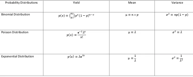
process capability index. Table 2 presents how to calculate the yield for different distributions.

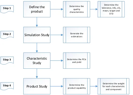
The flowchart in figure 4 summarizes all the steps required to determine the product

23

Table 2 Probability Distributions and their respective yield

Probability Distributions Yield Mean Variance

Binomial Distribution _{𝑝(𝑥) = (}𝑛

𝑥) 𝑝𝑥(1 − 𝑝)𝑛−𝑥 µ = 𝑛 ∗ 𝑝 𝜎

2_{= 𝑛𝑝(1 − 𝑝)}

Poisson Distribution

𝑝(𝑥) =е

−𝜆_𝜆𝑥

𝑥!

µ = 𝜆 𝜎2_{= 𝜆}

Exponential Distribution 𝑝(𝑥) = 𝜆е𝜆𝑥 _{µ =}1

𝜆 𝜎

2 ₌ 1

24

Define the

product

Simulation Study

Characteristic

Study

Product Study

Determine the quality characteristics

Generate the estimatiors

Determine the PCIs and yield

Determiine the product capability

Determine the tolerance, USL, LSL,

mean, target and STD

Determine the weight for each characteristic

and component

Step 1

Step 4 Step 2

Step 3

25

4. Results

The objective of this thesis is to determine the best approach to calculate the process

capability of products in the electronic industry. The results obtained will be presented following

the steps of the methodology.

4.1.Define the product

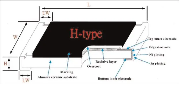
The product chosen for this study is the same one used by Ouyang, Hsu & Yang (2013)

in their paper. The product is the H-type chip resistor as show in the figure 4.

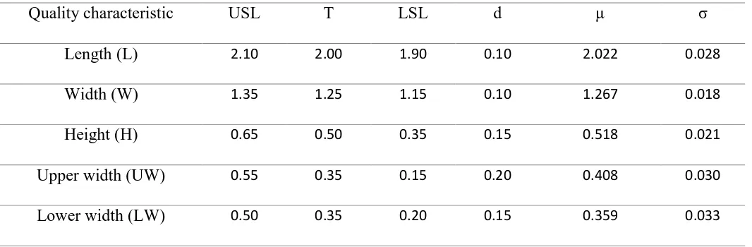
The characteristics analyzed are length, width, height, upper-width, and lower-width. The

mean, standard deviation, upper and lower specification limit, and the target are presented in the

table 3.

To apply the ideas presented in this paper, instead of considering the five quality

characteristic as part of one component, they will be analyzed in groups. The length, width, and

height will be analyzed as a quality characteristic of one component and the upper and lower

width as quality characteristic of another component. The final product is composed of these two

parts.

4.2.Simulation Study

The first step is to run the simulation; this is to determine the number of samples. In this

case, the sample size (n) is 761. The Appendix C presents how these values were calculated. To

run the simulation, it was ran using the Excel function NORMINV; this function generates

random numbers that follows the normal distribution. Appendix C also presents the steps on how

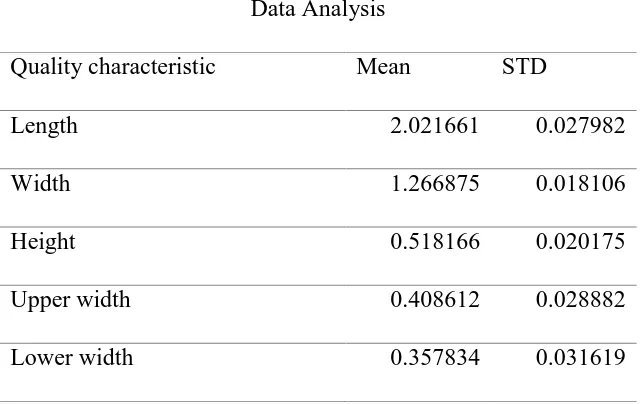
to use this function. Using this data, the estimators were calculated. Table 4 presents these values

26

For this study, the data obtained in the simulation must be in statistical control and follow

the normal distribution. Appendix D shows the test for these assumptions.

4.3.Characteristic Study

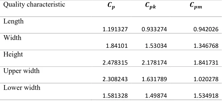
Using the data obtained in the last section, the 𝐶𝑝, 𝐶𝑝𝑘 and 𝐶𝑝𝑚 was calculated. Table 5

presents the results.

Using this data, it is also possible to determine the yields of the characteristics. The yield

was calculated using the method presented by Bothe (1992). Table 6 presents these results.

The yield was also calculated using the method presented by Chen & Huang, 2007. Table

7 presents the results obtained.

The Appendix E presents the equations that were used in this section.

4.4.Product Study

To calculate the product process capability, the yield and PCIs that were calculated in the

previous section were used. Aside from this, it is also necessary to determine the weight of each

characteristic. To do this, the first step is to determine what characteristics are more important.

4.4.1. Determining the weight (𝒘_𝒊)

For the quality characteristics of the product, we will assume that for the first component

the most important quality characteristic is the length (𝑘 = 10), followed by the height (𝑘 =

7) and then the width (𝑘 = 5). For the second component, the most important is the upper width

(𝑘 = 10), followed by the lower width (𝑘 = 8). Observing the components, the first (𝑘 = 9) is

27

28

Table 3 : Specification of the H-type chip resistor(unit: mm) (Ouyang et al., 2013)

Quality characteristic USL T LSL d µ σ

Length (L) 2.10 2.00 1.90 0.10 2.022 0.028

Width (W) 1.35 1.25 1.15 0.10 1.267 0.018

Height (H) 0.65 0.50 0.35 0.15 0.518 0.021

Upper width (UW) 0.55 0.35 0.15 0.20 0.408 0.030

29

Table 4: Mean and variance for the quality characteristic.

Data Analysis

Quality characteristic Mean STD

Length 2.021661 0.027982

Width 1.266875 0.018106

Height 0.518166 0.020175

Upper width 0.408612 0.028882

30

Table 5: PCIs for the quality characteristics

Quality characteristic 𝑪_𝒑 𝑪_𝒑𝒌 𝑪_𝒑𝒎

Length

1.191327 0.933274 0.942026

Width

1.84101 1.53034 1.346768

Height

2.478315 2.178174 1.841731

Upper width

2.308243 1.631789 1.020278

Lower width

31

Table 6 Yield for the quality characteristics

Quality characteristic Prod. Good using Bothe approach

Prod. Good using Chen & Huang approach Length

0.9974366 0.989537

Width

0.9999978 0.999984

Height

1 1

Upper width

0.9999995 0.999998

Lower width

32

4.4.2. Product capability using the PCIs

The first analysis follows the method presented by Mu at el (2009). The weight is

between 0 and 1. Table 7 presents the value of the weight of each characteristic as well as the

𝐶_𝑝𝑚𝑖𝑐 and 𝐶_𝑝𝑘𝑖𝑐 for each one of the components.

𝐶_𝑝𝑘𝑝 = 9 ∗ 𝐶𝑝𝑘1

𝑐 _{+ 10 ∗ 𝐶}

𝑝𝑘2𝑐

19 = 1.4938

𝐶_𝑝𝑚𝑝 = 9 ∗ 𝐶𝑝𝑚1

𝑐 _{+ 10 ∗ 𝐶}

𝑝𝑚2𝑐

19 = 1.261455

To determine the influence of the use of the weights, it is necessary to repeat this analysis

and use the characteristics and components with the same weight. The results are presented in

table 8.

Using the results presented in Table 8, it is possible to determine the product capability

indices.

𝐶_𝑝𝑘𝑝 = 1 ∗ 𝐶𝑝𝑘1

𝑐 _{+ 1 ∗ 𝐶}

𝑝𝑘2𝑐

2 = 1.556264

𝐶_𝑝𝑚𝑝 =1 ∗ 𝐶𝑝𝑚1

𝑐 _{+ 1 ∗ 𝐶}

𝑝𝑚2𝑐

2 = 1.32722

The first analysis follows the method presented by Yu et al. (2007). In this case, the

weight is between 1 and 5. Table 9 presents the weight for each one of the characteristics and

also the 𝐶_𝑝𝑚𝑖𝑐 and 𝐶_𝑝𝑘𝑖𝑐 for each one of the components.

𝐶_𝑝𝑘𝑝 = √𝐶𝑐

𝑝𝑚14.5∗ 𝐶𝑝𝑚25

(4.5+5)

= 1.449035

𝐶_𝑝𝑚𝑝 = √𝐶𝑝𝑘14.5∗ 𝐶𝑐𝑝𝑘25

(4.5+5)

33

Table 7 Process capability for the components using the PCIs

Quality characteristic Weight (𝒘_𝒊) 𝑪_𝒑𝒌𝒊 𝑪_𝒑𝒌𝒊∗ 𝒘_𝒊 𝑪_𝒑𝒎𝒊 𝑪_𝒑𝒎𝒊∗ 𝒘_𝒊

Length

0.454545 0.933274 0.424215 0.942026 0.428194

Width

0.318182 1.53034 0.486926 1.346768 0.428517

Height

0.227273 2.178174 0.49504 1.841731 0.418575

First Component 𝐶_𝑝𝑘1𝑐 = 1.406181

𝐶_𝑝𝑚1𝑐 = 1.275286 Upper width

0.555556 1.631789 0.90655 1.020278 0.566821

Lower width

0.444444 1.49874 0.666107 1.534918 0.682186

Second Component 𝐶_𝑝𝑘2𝑐 = 1.572656 _𝐶

34

Table 8 Process capability for the components using the PCIs (without weight)

Quality characteristic Weight (𝒘_𝒊) 𝑪_𝒑𝒌𝒊 𝑪_𝒑𝒌𝒊∗ 𝒘_𝒊 𝑪_𝒑𝒎𝒊 𝑪_𝒑𝒎𝒊∗ 𝒘_𝒊

Length 0.333333 0.933274 0.311091 0.942026 0.314009

Width 0.333333 1.53034 0.510113 1.346768 0.448923

Height 0.333333 2.178174 0.726058 1.841731 0.61391

First Component 𝑪_𝒑𝒌𝟏 1.547263 𝑪𝒑𝒎𝟏 1.376842

Upper width 0.5 1.631789 0.815895 1.020278 0.510139

Lower width 0.5 1.49874 0.74937 1.534918 0.767459

35

Table 9 Process capability for the components using the yield

Quality characteristic Weight (𝒘_𝒊) 𝑪_𝒑𝒌𝒊 𝑪_𝒑𝒌𝒊𝒘𝒊 _𝑪

𝒑𝒎𝒊 𝑪𝒑𝒎𝒊𝒘𝒊

Length

5 0.933274 0.70802 0.942026 0.741847

Width

3.5 1.53034 4.433611 1.346768 2.834815

Height

2.5 2.178174 7.002153 1.841731 4.60326

First Component 𝐶_𝑝𝑘1𝑐 =

1.324351 𝐶𝑝𝑚1𝑐 = 1.229214

Upper width

5 0.933274 0.70802 0.942026 0.741847

Lower width

4 1.53034 4.433611 1.346768 2.834815

Second Component

5 𝐶𝑝𝑘2 𝑐 ₌

36

To determine the influence of the use of the weight, it is necessary to repeat this analysis

and use the characteristics and components with the same weight. The results are presented in

table 10.

Using the PCI for the first and second components presented in the Table 10, it is

possible to determine the product capability.

𝐶_𝑝𝑘𝑝 = √𝐶𝑐

𝑝𝑚11∗ 𝐶𝑝𝑚21

2

= 1.510935

𝐶_𝑝𝑚𝑝 = √𝐶_𝑝𝑘11∗ 𝐶𝑐 𝑝𝑘21

2

= 1.288639

4.4.3. Process capability using the yield

Using the yield obtained in the table 6 it is possible to determine the product yield. Using

this value and the data presented in the Appendix A and B it is possible to determine the 𝐶_𝑝𝑘𝑝 and

the 𝐶_𝑝𝑚𝑝 .

For the 𝐶_𝑝𝑘𝑝 , the yield used is obtained by the product of the data presented in the table 6

𝑌_𝐶𝑝𝑘𝑝 = 99.7426

Using this value and the data presented in Appendix A, we have that

𝐶_𝑝𝑘𝑝 = 1.45

For the 𝐶_𝑝𝑚𝑝 , the yield used is obtained by the product of the data presented in the table 7

𝑌_𝐶𝑝𝑘𝑝 = 98.94

Using this value and the data presented in the Appendix B, we have that

37

Table 10 Process capability for the components using the yield (without weight)

Quality characteristic Weight (𝒘𝒊) 𝑪𝒑𝒌𝒊 𝑪𝒑𝒌𝒊𝒘𝒊 𝑪𝒑𝒎𝒊 𝑪𝒑𝒎𝒊𝒘𝒊

Length

0.33 0.933274 0.966061 0.942026 0.97058

Width

0.33 1.53034 1.237069 1.346768 1.160503

Height

0.33 2.178174 1.475864 1.841731 1.357104

First Component 𝐶_𝑝𝑘1𝑐 =

1.459811 𝐶𝑝𝑚1𝑐 = 1.326968

Upper width

0.5 1.631789 1.277415 1.020278 1.010088

Lower width

0.5 1.49874 1.22423 1.534918 1.238918

Second Component 𝐶_𝑝𝑘2𝑐 =

1.56385 𝐶𝑝𝑚2

𝑐 ₌

38

5. Discussion

To better analyze the results, the discussion will be divided into three parts. The first one

presents the discussion of the simulation results, the second presents the quality characteristic

study results analyses and the third presents the product study results analyses.

5.1.Simulation Analyses

To determine if the data obtained in the simulation is accurate, it is necessary to compare

the values obtained for the mean and standard deviation with the historical values. Table 11

presents the results obtained for the µ, σ, 𝑋̅ and 𝑆. Also, the table presents the error for this data.

The results presented in Table 11 of the simulation is accurate. For the mean, all of the

errors are less than 1%, so the data generated presents values close to the mean. For the standard

deviation, the errors are less than 5%for four characteristics, and the 𝑺is smaller than the

historical standard deviation.

5.2.Quality Characteristics Analyses

The process capability indices are used to determine if a process is capable of meeting the

specification, Table 12 presents 𝐶𝑝, 𝐶𝑝𝑘 and 𝐶𝑝𝑚 values. Looking at this table, all of the quality

characteristics has the 𝐶_𝑝 as the biggest value This happen because this CPI doesn’t analyze the

departure of the mean from the target as well as the distribution of the sample. If the mean is not

equal to the target, the 𝐶𝑝 will induce a wrong acceptance of the process. Figure 5 shows that all

the characteristics presented are off target.

The 𝐶_𝑝 doesn’t analyze how the mean is located in relationship to the specification limits.

If the distance between the mean to the upper and lower specification limit is different, the 𝐶𝑝

39

𝐶_𝑝𝑘 is more sensitive to how the data is spread and also to the location of the mean

relative to the specification limits. The 𝐶_𝑝𝑚 is more sensitive to the mean departure from the

target. Table 12 shows the variability between the mean and the target as well as the variability

between the mean and the specification limits.

Analyzing table 12 it is possible to conclude that the upper width presents the biggest

variance between the mean and the target, due to this, the 𝐶_𝑝𝑚 presents a smaller value. Lower

width and the length present similar values for the 𝐶_𝑝𝑚 and 𝐶_𝑝𝑘; this happens because the

variability between the mean and target is small and the distance between the mean and the

specifications limits are close.

Even with the variability between the mean and the target (being lower for the width), the

mean is not centered between the specifications limits, so the 𝐶𝑝𝑚 also presents a small value.

For the height, the variance between the mean and target and the distance between the mean and

40

Table 11 Comparison between the real data and the simulation data

Quality Characteristic µ 𝒙̅ error (%) σ 𝑺 error (%)

Length

2.02200

2.02166 0.01677 0.02800 0.02798 0.07143

Width

1.26700

1.26688 0.00987 0.01800 0.01811 0.58889

Height

0.51800

0.51817 0.03205 0.02100 0.02018 3.92857

Upper width

0.40800

0.40861 0.15000 0.03000 0.02888 3.72667

Lower width

0.35900

41

Table 12 Quality characteristics summary results

Quality characteristic

µ T µ − 𝑻

µ ∗ 𝟏𝟎𝟎

USL USL- µ LSL µ-LSL 𝑪_𝒑 𝑪_𝒑𝒌 𝑪_𝒑𝒎

Length 2.021661 2 1.071446 2.1 0.078339 1.9 0.121661 1.191327 0.933274 0.942026

Width 1.266875 1.25 1.332018 1.35 0.083125 1.15 0.116875 1.84101 1.53034 1.346768

Height 0.518166 0.5 3.505826 0.65 0.131834 0.35 0.168166 2.478315 2.178174 1.841731

Upper width 0.408612 0.35 1.434417 0.55 0.141388 0.15 0.258612 2.308243 1.631789 1.020278

42

43

5.3.Product Capability Analyses

The product capability analyzes the capability of a product to meet the quality standard

required. To determine this, it is necessary to analyze the quality characteristics and the

components of the product. In this project, the product capability was determined using the PCIs

and the yield.

Using the PCIs, the product capability was determined with and without the influence of

weight in the quality characteristics. Table 13 summarizes the results obtained in this study.

Observing the results presented in table 13, it is possible to arrive to some conclusions.

First, the use of the weight will impact in the product capability. The difference between the PCI

with and without the use of the influence of the quality characteristic shows the importance of

this study. The use of the weight results in a more accurate PCI value because in a manufacturing

process a product is composed of different components and each one will have a different

influence in the final quality of the product. Using the weight first will allow to determine if each

characteristic is critical. Secondly, it will help in determining where the investment must be done

to improve the product quality.

In analyzing the 𝐶_𝑝𝑘 and the𝐶_𝑝𝑚 values, he 𝐶_𝑝𝑚 is smaller than the 𝐶_𝑝𝑘. This shows that

the use of the 𝐶_𝑝𝑘 to analyze the product capability can lead to a wrong acceptance of the

product.

Using the yield to determine the product capability, we have that the 𝐶_𝑝𝑘𝑝 is equal to 1.45

and the 𝐶_𝑝𝑚𝑝 is equal to 0.95. Observing the results presented in the table 14, it is possible to

conclude that the use of the yield to determine the 𝐶_𝑝𝑘𝑝 is accurate, but to determine the 𝐶_𝑝𝑚𝑝 this

approach will present some errors. This happens because for the 𝐶_𝑝𝑘𝑝 , the value of the yield will

44

Table 13 Product capability using the PCI of the characteristics and components

Chen and Huan approach Yu et al approach

With 𝑤𝑖 Without 𝑤𝑖 With 𝑤𝑖 Without 𝑤𝑖

𝑪_𝒑𝒌 1.4938 1.556264 1.449035 1.510935

45

6. Conclusion

Observing everything that was presented in this thesis, it is possible to conclude a few

things:

 The use of the Monte Carlo simulation to generate data when the real data of the

process is not available is accurate. When the deviation of mean and standard

deviation value is small, the random data created can be used to determine the

estimators of the sample.

 To determine the PCIs values, the data must be in control and must follow the

normal distribution, if the data doesn’t attend this assumption, the use of the PCIs

is not possible.

 Between the process capability indices presented, the 𝐶_𝑝𝑚 will lead to more

accurate results because analyzing the variability of the data also presents high

sensibility to the mean deviation from the target. The use of the 𝐶_𝑝 and the 𝐶_𝑝𝑘 for

the process of a target will result in the wrong acceptance of the process.

 To determine the capability of the product, it is necessary to firs determine the

influence of each quality characteristic in the final quality of the component that

composes the product. Lastly, it is then necessary to also determine the weight of

the component. Using this weight, the product capability will be more accurate

and also, this will help determine the right place as to where to invest in order to

result in a higher improvement of quality.

 There are two approaches to apply to the weight of the process capability. One

uses the sum and the other uses the product. For this study, any of the approaches

46

 The use of the yield to determine the product capability is accurate when the

process capability index analyzed is the 𝐶𝑝𝑘, for the 𝐶𝑝𝑚 . The use of the yield can

lead to the wrong results.

 To analyze a process that doesn’t follow the normal distribution, the use of the

yield is a good option. It’s not possible to determine the process capability index,

but it is possible to determine the range of parts that meet the specification, which

47

7. Reference

Bothe, D. R. (1992). A Capability Study for an Entire Product. Annual Quality Congress, 46(0).

Chan, L. K., Cheng, S. W., & Spiring, F. A. (1988). A new measure of process capability: Cpm.

Journal of Quality Technology, 20(3).

Chen, K. S., & Huang, M. L. (2007). Process Capability Evaluation for the Process of Product

Families. Quality & Quantity, 41(1), 151-162. doi:10.1007/s11135-005-6223-7

Chen, K. S., Huang, M. L., & Li, R. K. (2001). Process capability analysis for an entire product.

International Journal of Production Research, 39(17), 4077-4087.

doi:10.1080/00207540110073082

Driels, M. R., & Shin, Y. S. (2004). Determining the Number of Iterations for Monte Carlo

Simulations of Weapon

Effectiveness. Retrieved from

Hsiang, T. C., & Taguchi, G. (1985). A tutorial on quality control and assurance — the Taguchi

methods. Las Vegas, Nevada: Annual Meetings of the American Statistical Association.

Huang, W., & Kong, Z. (2010). Process Capability Sensitivity Analysis for Design Evaluation of

Multistage Assembly Processes. IEEE Transactions on Automation Science and

Engineering, 7(4), 736-745. doi:10.1109/TASE.2009.2034633

Juran, J. M., Bingham, R. S., & Gryna, F. M. (1974). Quality control handbook (Vol. 3d). New

York: McGraw-Hill.

Kane, V. E. (1986). Process capability indices. 18(1), 41-52. .

Kureková, E. (2001). Measurement Process Capability – Trends and Approaches.

MEASUREMENT SCIENCE REVIEW, 1(1).

48

Mu, W., He, Y., Chang, W., & Ma, Z. (2009, 2009). A study on comprehensive evaluation model

of product producing process capability.

Ouyang, L.-Y., Hsu, C.-H., & Yang, C.-M. (2013). A new process capability analysis chart

approach on the chip resistor quality management. Proceedings of the Institution of

Mechanical Engineers, Part B: Journal of Engineering Manufacture, 227(7), 1075-1082.

Pearn, W. L., & Chen, K. S. (1997). Capability indices for non-normal distributions with an

application in electrolytic capacitor manufacturing. Microelectronics Reliability, 37(12),

1853-1858. doi:10.1016/S0026-2714(97)00023-1

Shewhart, W. A. (1939). Statistical method from the viewpoint of quality control.

Singhal, S. C. (1990). A New Chart for Analyzing Multi Process Performance. Quality

Engineering, 2(4).

Singhal, S. C. (1992). Miltiprocess Performance Analysis Chart (MPPAC) With Capability

Zones. Quality Engineering, 4(1).

Spence, R. (1984). Tolerance analysis and design of electronic circuits. Computer-Aided

Engineering Journal, 1(3), 91. doi:10.1049/cae.1984.0010

Wu, C.-W., Pearn, W. L., & Kotz, S. (2009). An overview of theory and practice on process

capability indices for quality assurance. International Journal of Production Economics,

117(2), 338-359. doi:http://dx.doi.org/10.1016/j.ijpe.2008.11.008

Wu, C. C., Kuo, H. L., & Chen, K. S. (2004). Implementing process capability indices for a

complete product. The International Journal of Advanced Manufacturing Technology,

49

Yu, K. T., Sheu, S. H., & Chen, K. S. (2007). Testing multi-characteristic product capability

indices. The International Journal of Advanced Manufacturing Technology, 34(5),

421-429. doi:10.1007/s00170-006-0598-z

Zhai, G., Zhou, Y., Ye, X., & Hu, B. (2013). A method of multi-objective reliability tolerance

design for electronic circuits. Chinese Journal of Aeronautics, 26(1), 161-170.

50

Appendix A: Yield to Process Capability Conversion (𝑪_𝒑𝒌)

Yield % Sigma 𝑪𝒑𝒌

6.70% 0 0

15.90% 0.5 0.17

30.90% 1 0.33

50.00% 1.5 0.5

69.10% 2 0.67

84.10% 2.5 0.83

93.30% 3 1

97.70% 3.5 1.17

99.40% 4 1.33

99.87% 4.5 1.5

99.98% 5 1.67

99.9968% 5.5 1.83

51

Appendix B: Yield values for different 𝑪_𝒑𝒎

Com h

1 2 3 4 5 6 7 8 9 10

0,05 0,00000 0,00002 0,00357 0,02383 0,05499 0,08266 0,10163 0,11264 0,11785 0,11924

0,10 0,00000 0,00034 0,01462 0,06045 0,11896 0,16895 0,20335 0,22354 0,23322 0,23582

0,15 0,00000 0,00404 0,04650 0,12143 0,19845 0,26122 0,30481 0,33096 0,34378 0,34729

0,20 0,00004 0,02878 0,11904 0,21431 0,29566 0,35963 0,40500 0,43319 0,44748 0,45149

0,25 0,00715 0,12528 0,24832 0,33858 0,40763 0,46190 0,50219 0,52861 0,54265 0,54675

0,30 0,17109 0,34495 0,42866 0,48353 0,52688 0,56388 0,59413 0,61577 0,62810 0,63188

0,35 0,70888 0,63721 0,62559 0,63070 0,64348 0,66052 0,67845 0,69353 0,70312 0,70628

0,40 0,97982 0,86456 0,79395 0,76075 0,74790 0,74708 0,75306 0,76115 0,76750 0,76986

0,45 0,99981 0,96792 0,90662 0,86075 0,83346 0,82017 0,81656 0,81835 0,82150 0,82298

0,50 1,00000 0,99535 0,96564 0,92768 0,89759 0,87826 0,86843 0,86537 0,86573 0,86639

0,55 1,00000 0,99960 0,98984 0,96665 0,94155 0,92169 0,90901 0,90287 0,90110 0,90106

0,60 1,00000 0,99998 0,99760 0,98640 0,96912 0,95220 0,93941 0,93184 0,92871 0,92814

0,65 1,00000 1,00000 0,99955 0,99511 0,98492 0,97236 0,96119 0,95353 0,94974 0,94882

0,70 1,00000 1,00000 0,99993 0,99846 0,99321 0,98487 0,97611 0,96923 0,96535 0,96427

0,75 1,00000 1,00000 0,99999 0,99957 0,99718 0,99217 0,98587 0,98024 0,97666 0,97555

0,80 1,00000 1,00000 1,00000 0,99990 0,99892 0,99617 0,99198 0,98769 0,98464 0,98360

0,85 1,00000 1,00000 1,00000 0,99998 0,99962 0,99823 0,99564 0,99256 0,99013 0,98923

0,90 1,00000 1,00000 1,00000 1,00000 0,99988 0,99923 0,99772 0,99565 0,99381 0,99307

0,95 1,00000 1,00000 1,00000 1,00000 0,99996 0,99968 0,99886 0,99753 0,99621 0,99563

1,00 1,00000 1,00000 1,00000 1,00000 0,99999 0,99988 0,99945 0,99865 0,99774 0,99730

1,05 1,00000 1,00000 1,00000 1,00000 1,00000 0,99996 0,99975 0,99928 0,99868 0,99837

1,10 1,00000 1,00000 1,00000 1,00000 1,00000 0,99998 0,99989 0,99963 0,99925 0,99903

52

1,20 1,00000 1,00000 1,00000 1,00000 1,00000 1,00000 0,99998 0,99991 0,99978 0,99968

1,25 1,00000 1,00000 1,00000 1,00000 1,00000 1,00000 0,99999 0,99996 0,99988 0,99982

1,30 1,00000 1,00000 1,00000 1,00000 1,00000 1,00000 1,00000 0,99998 0,99994 0,99990

1,35 1,00000 1,00000 1,00000 1,00000 1,00000 1,00000 1,00000 0,99999 0,99997 0,99995

1,40 1,00000 1,00000 1,00000 1,00000 1,00000 1,00000 1,00000 1,00000 0,99999 0,99997

1,45 1,00000 1,00000 1,00000 1,00000 1,00000 1,00000 1,00000 1,00000 0,99999 0,99999

1,50 1,00000 1,00000 1,00000 1,00000 1,00000 1,00000 1,00000 1,00000 1,00000 0,99999

1,55 1,00000 1,00000 1,00000 1,00000 1,00000 1,00000 1,00000 1,00000 1,00000 1,00000

1,60 1,00000 1,00000 1,00000 1,00000 1,00000 1,00000 1,00000 1,00000 1,00000 1,00000

1,65 1,00000 1,00000 1,00000 1,00000 1,00000 1,00000 1,00000 1,00000 1,00000 1,00000

1,70 1,00000 1,00000 1,00000 1,00000 1,00000 1,00000 1,00000 1,00000 1,00000 1,00000

1,75 1,00000 1,00000 1,00000 1,00000 1,00000 1,00000 1,00000 1,00000 1,00000 1,00000

1,80 1,00000 1,00000 1,00000 1,00000 1,00000 1,00000 1,00000 1,00000 1,00000 1,00000

1,85 1,00000 1,00000 1,00000 1,00000 1,00000 1,00000 1,00000 1,00000 1,00000 1,00000

1,90 1,00000 1,00000 1,00000 1,00000 1,00000 1,00000 1,00000 1,00000 1,00000 1,00000

1,95 1,00000 1,00000 1,00000 1,00000 1,00000 1,00000 1,00000 1,00000 1,00000 1,00000

53

Appendix C: Simulation Study

To calculate the sample size, it is necessary to know the confidence level required, the

error acceptable, the standard deviation, the mean and how the product studied presents a tight

tolerance. The confidence level will be 99.75%, which gives a 𝑧 = 3 , and the error will be 1%

for all the characteristics. The table below presents the data used and the sample size for each

characteristic.

Quality characteristic z e µ σ n

Length (L) 3 1 2.022 0.028 18.0

Width (W) 3 1 1.267 0.018 19.0

Height (H) 3 1 0.518 0.021 148.0

Upper width (UW) 3 1 0.408 0.030 487.0

Lower width (LW) 3 1 0.359 0.033 761.0

To use the excel function NORMINV, these steps must to be followed:

 Determine the function input

o Mean

o Standard deviation

 Write the function = NORMINV(rand();mean; standard deviation)

 Select the cells that you want to save (the result of the simulation) and the

cell with the number of runs

 Go to Data – What If Analysis – Data table

 For the Column/Row input cell: select any empty cell

 Click OK

54

Appendix D: Data Assumption Test

To use the process capability indices, the data must be in statistical control and must

follow the normal distribution. To check the normal distribution assumption, it is necessary to