Analysis and hardware implementation of color map inversion algorithms

Rochester Institute of Technology

RIT Scholar Works

Theses

Thesis/Dissertation Collections

8-1-2002

Analysis and hardware implementation of color

map inversion algorithms

Michael Martin

Follow this and additional works at:

http://scholarworks.rit.edu/theses

This Thesis is brought to you for free and open access by the Thesis/Dissertation Collections at RIT Scholar Works. It has been accepted for inclusion in Theses by an authorized administrator of RIT Scholar Works. For more information, please [email protected].

Recommended Citation

Analysis and Hardware Implementation of

Color Map Inversion Algorithms

by

Michael W. Martin

A Thesis Submitted in Partial Fulfillment

of the Requirements for the Degree of

MASTER OF SCIENCE

Computer Engineering

Approved By:

Principal Advisor

Kenneth Hsu, Professor, Computer Engineering

Committee Member

-Soheil Dianat, Professor, Electrical Engineering

Committee Member

_

Athimoottil Mathew, Professor, Electrical Engineering

Department Head

Andreas Savakis, Associate Professor and Department Head, Computer Engineering

Department of Computer Engineering

College of Engineering

Rochester Institute of Technology

Rochester, New York

REPRODUCTION PERMISSION STATEMENT

PERMISSION DENIED

Analysis and Hardware Implementation of

Color Map Inversion Algorithms

I, Michael W. Martin, hereby deny permission to any individual or organization to

reproduce this thesis in whole or in part.

Michael W. Martin

Abstract

Thepurposeofthis thesis isto investigateseveral algorithmsthatare usedto computethe

inverse of a forward printer map. The forward printer _map models the printer

by

mapping points in the printer's input color space to points in the printer's output color

space. The inverseofthis forward_map isrequiredto convertinputcolor specificationsin

adevice-independentcolor spaceto a colorin the printer's device-dependentcolor space

before

being

presented to the print engine. The accuracy of the inverse printer _map

directly

affects the _accuracy ofthe reproduced colors.

Therefore,

_anymeasured change

in the forward printer _map requires re-computation ofthe _{inverse map if} accurate and

consistent color reproduction is to be maintained. An efficient and accurate method of

computingtheinverse map couldbeusedinan automaticcolor correction system.

Three algorithms for computingtheinverse ofthe forwardprinter_map arestudiedinthis

thesis project. These are the

Shepard's,

Moving

Matrix,

and

Iteratively

Clustered

Interpolation

(ICI)

algorithms. The algorithms are implemented in C and simulated in

ordertobenchmarktheirrelativeaccuracy, speed, and complexity. The simulations show

the ICI algorithmto be the fastest and most accurate at _computing the inverse map, and

its _{complexity does} not far exceed that ofthe other algorithms. The ICI algorithm was

implemented in VHDL and synthesized to a Synopsys generic

library

in order to

determine the approximate size and speed of an ASIC that could perform the inverse

computation. The finalimplementationresultedintwomodules: onethatimplementsthe

ICI _algorithm, andonethat implementsthetrilinearinterpolation functionthat isused

by

synthesized trilinear interpolation module contained 190,357 cells. The

timing

ofthe

modules resulted in a 40 nanosecond clock _period, which corresponds to a maximum

operating

frequency

of25 MHz. These synthesized results show that this algorithm is

Table

of

Contents

1 INTRODUCTION

2 BACKGROUND INFORMATION

2.1 The XerographicPrinting Process 3

2.2 Color Spaces 4

2.2.1 RGBColor Space 4

2.2.2 CMY Color Space 4

2.2.3 LAB Color Space 6

2.3 Gamut Mapping 7

3 DEVICE MODELING 10

3.1 Forward Printer Map 11

3.2 Inverse Printer Map 12

4 THEORY 13

4.1 Algorithms 16

4.1.1 Shepard's Algorithm 17

4.1.2 Moving Matrix Algorithm 18

4.1.3 Iteratively Clustered Interpolation Algorithm 19

4.1.4 Trilinear Interpolation 23

5 SOFTWAREIMPLEMENTATION 25

5.1 Algorithm Metrics 25

5.1.1 DeterminingAlgorithm Complexity 25

5.1.2 DeterminingAlgorithmExecution Speed 26

5.1.3 DeterminingAlgorithm Accuracy 26

5.2 OptimalParameters 27

5.2.1 Shepard'sAlgorithm 28

5.2.2 Moving Matrix Algorithm 28

5.2.3 ICI Algorithm 28

5.3 Simulation Results 30

6 ICI HARDWAREIMPLEMENTATION 32

6.1 Design Methodology 32

6.1.2 Datastorage 33

6.1.2.1 Operation 34

6.1.2.2

Memory

Data Layout 35

6.1.3 Data Representation ₃₆

6.2 Synthesis Methodology 37

6.3 Simulation&Testing ₃₉

6.4 Hardware Modules 40

6.4.1 TrilinearInterpolation Module

(tritop.vhd)

40

6.4.1.1 Operation 42

6.4.1.2 Sub-blocks 43

6.4.1.3

Summary

ofResults 50

6.4.2 ICIModule

(icitop.vhd)

51

6.4.2.1 Operation 55

6.4.2.2 Input Description 55

6.4.2.3 Sub-blocks 56

6.4.3 SummaryofResults 63

6.5 SystemOverview 63

7 CONCLUDING REMARKS 65

7.1 Conclusions 65

7.2 Future Work 66

7.3 Acknowledgements 66

8 REFERENCES 68

9 APPENDICES 69

9.1 Software Simulation accuracy Results 69

9.1.1 Shepard'sInterpolation 70

9.1.2 Moving Matrix 71

9.1.3 ICI 71

9.2 VHDL Code 73

9.2.1 TRIJTOP.VHD 73

9.2.2 TRI_CTRL.VHD 77

9.2.3 TRICXBLOCK.VHD 84

9.2.4 TRI_TERM_BLOCK.VHD 85

9.2.5 TRI_ADDRJBLOCK.VHD 86

9.2.6 TRI_TB_TOP.VHD 87

9.2.7 ICITOP.VHD 89

9.2.8 ICI_CTRL.VHD 93

9.2.9 ICIJDP.VHD 103

9.2.10 DIS_DP.VHD 104

9.2.11 ADDR_CALC.VHD 105

List

of

Figures

Figure 1: The Xerographic

Printing

Process 3

Figure 2: AxesoftheCIELAB color space ₆

Figure 3: Gamut

Mapping

for Constant LightnessandHue ₁₀

Figure 4: Systemof P"1

andP ₁₄

Figure 5: Sub-cubewith_{Lattice Points Determined}

During

_{Extraction 23}

Figure 6: ID LinearInterpolation ₂₄

Figure 7:

Memory

Module Diagram 34

Figure 8:

Top

Level DiagramofTrilinearInterpolationModule 40

Figure 9: Submodule DiagramofTrilinearInterpolationModule 41

Figure 10:

Top

LevelDiagramof_{Trilinear Interpolation TRICTRL Block 44}

Figure 11:

Top

Level Diagramof_{Trilinear Interpolation TRIADDRBLOCK} 45

Figure 12: DatapathArchitectureofTRIADDRBLOCK 46

Figure 13:

Top

Level Diagramof_{Trilinear Interpolation TRICXBLOCK} 47

Figure 14: DatapathArchitectureofTRI_CX_BLOCK 47

Figure 15:

Top

Level Diagramof_{Trilinear Interpolation TRI_TERM_BLOCK} 48

Figure 16: Datapath ArchitectureofTRITERMBLOCK 49

Figure 17:

Top

Level Diagram ofICI Module 51

Figure 18: Submodule DiagramofICI Module 52

Figure 19:

Top

Level DiagramofICI_CTRL Block 57

Figure 20:

Top

Level Diagram ofICIADDRCALCBlock 58

Figure 21: Datapath ArchitectureofICIADDRCALCBlock 58

Figure 22:

Top

Level Diagram ofICI DIS_DP Block 59

Figure 23: Datapath ArchitectureofICI DISDP Block 60

Figure 24:

Top

Level DigramofICIDP Block 61

Figure 25: Datapath ArchitectureofICIJDPBlock 62

Figure 26: DiagramofSystemto Compute P"

64

List

of

Tables

Table 1:

Optimal

AlgorithmParameters 29

Table 2: Algorithm

Accuracy

30

Table 3: Algorithm Execution Time 30

Table 4: Algorithm

Complexity

30

Table5: Trilinear Interpolation Module I/O Signals 42

Table6: Trilinear Interpolation ModuleSynthesisResults 50

Table 7: ICIModule I/OSignals 53

1

Introduction

One of the most crucial challenges

facing

today's printer manufacturers is to design

printers that _accurately and _consistently reproduce the colors in images [1]. This is a

difficulttaskbecause the transformation fromtheprinter'sinput color spaceto its output

color space isnon-linear and drifts overtime. Colorreproductionis also affected

by

the

physicalproperties of_{the media,}

including

temperature,

moisture _content,

brightness,

and

weight. These variables are _{constantly changing} and can lead to inaccurate and

inconsistentcolorreproduction. Whenthis occurs,theprinter mustbere-calibrated. The

calibrationprocess is

typically

manual and

time-consuming

and reduces the_productivity

oftheprinter.

Acolor correction system is neededto account forthese variationsin orderto _accurately

and_consistentlyreproduce thecolors inprintedimages. Solutions that can automatethe

color correction process will lead to _very productive printers with little "downtime".

There is an abundance of research activity aimed at

developing

efficient and effective

colorcalibration and control systems

[6, 8,

10]. The forward andinverseprintermaps are

centralto_manyofthesesystems.

A forward printer_map is apractical and accurate model ofaprinter. This forward map

takes the form of a multidimensional

look-up

table and is constructed

by

performing

input-output color experiments on an actual printer. The inverse ofthis forward map,

called the inverse printer map, is needed to convert an input color specification in a

before

being

presentedto theprint engine. Ifthe

inverse

printer_mapis _{accurate, the}print

engine will produce a color reproduction that _closely matches the original

device-independent color specification.

Any

measured change in the forward printer _map

requires re-computation ofthe inverse _map if color _accuracy and _consistency is to be

maintained. A method for _accurately and _{efficiently computing} the inverse of the

forward map issought.

Section 1 ofthis paper is this briefintroduction. In Section

2,

several important topics

relating to this project will be discussed. Section 3 describes howprinters are modeled.

Section 4presentstheproblem athand andthe

theory

behindtheproblem. Theinversion

algorithms are also discussed in this chapter. Section 5 describes the software

implementation and results. Section 6 describes the hardware implementation and

results.

Finally,

Section 7 concludes the paper with a discussion ofconclusions, future

work, and acknowledgements. ReferencesandAppendices canbe foundattheend ofthe

paper. The CD accompanying this paper includes the paper itselfas well as data

files,

2

Background Information

2. 1

The

Xerographic

Printing

Process

Imaging

systems consist of a network _{consisting primarily} of video

display

monitors,

scanners, and printers. Each ofthese devices havetheir owndevice-specific color _space;

generally RGB for monitors and scanners and CMY for printers. These devices

communicate image data with each other _using a psycho-physical based and

device-independentcolor_space, suchas LAB.

Aspecificationinthedevice-independentcolor spaceistransformedintoa

device-dependentcolor space _usingamultidimensional color correctiontableorinversecolor

map. Thisinverse _mapisbasedontheforwardtransformationcharacteristicsofthe

printer. Onceconvertedintothedevice-dependentcolor_space,thecolor-separatedimage

isconvertedto halftonesanddeliveredto theprintenginethatisresponsibleforthe

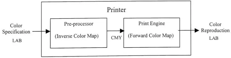
physical productionoftheprint [8]. Thisprocessisillustrated in Figure 1.

Color

Specification

LAB

Printer

Pre-processor

(Inverse Color_{Map) CMY}

Print Engine

(ForwardColorMap)

Color

-?Reproduction

[image:12.499.42.434.489.588.2]

LAB

2.2

Color

Spaces

Coloris specified inathree

dimensional

space where each point inthe space describesa

single color. There are several such color _spaces, such as

RGB, CMY,

and LAB. This

project focuses on _printers;

therefore,

_{this research work was}

done using the CMY and

LAB color spaces described in this section. The RGB color space is also described in

order to further explain and contrast the additive and subtractive nature ofthe color

systems. Although not used

directly

in the _{printing process,} RGB is the color system

used on the displays that show the images prior to _printing and to which the color

reproductionis often compared.

2.2.1

RGB

Color Space

IntheRGB _space, a color consists ofthe_primarycomponents_{red, green,} andblue. The

RGB system is _{additive, meaning} that _varying amounts of the primaries are added

together to produce agiven color. The additive nature ofthe RGB system makes it the

color system of choice for devices that are _{self-illuminating light sources,} such as

displays and scanners. This color space is known as a device-dependent color space

becausethesameRGB colorspecificationwill_{vary perceptually}ondifferent devices.

2.2.2

CMY Color Space

Another device-dependent color space isthe CMY space. A colorin this space consists

meaningthat_varyingamounts oftheprimaries are used together to absorbcertaincolors;

thosecolorsthatare_reflected,ratherthan_absorbed,combineto formtheperceived color.

Colorprints are illuminated

by

an external light _source, and theperceived colors aredue

to the combination of reflected wavelengths.

Thus,

a printer's input color space is

typically

described in CMY.

Printers

typically

add a fourth ink

-black

-which results in four-color CMYK. The

black ink is addedforseveral reasons. Toproduce_{black using only}theCMYprimaries,

100percent ofeachinkmustbeused. Thisisadisadvantagebecausecolorinksare more

expensive andbecause_{using 100}percentofthe threeprimariesresults ina_verywet print

thatis susceptibleto wrinkles andtakesa

long

time todry.

Furthermore,

thecombination

offull CMY usuallyresults inmore of a_{muddy brown} thanblack color.

Also,

because

the _overlayof_{inks may}notbeexact,blackportions of a print_{may have} edgesthatdonot

have full CMY coverage. Ifthese reasons are not enough,

including

black in the color

mix can increase the contrast of colors

thereby

increasing

a printer's color gamut.

Replacing

some percentage of the three primaries is achieved

by

_gray component

replacement and under color removal [7]. A color can be specified _{using only} these

primaries; theblack component is addedlater

by

a separate and independent _processing

step. In _{this project,} we need _only consider the three primaries _{cyan, magenta,} and

2.2.3

LAB

Color Space

The LAB

(CIELab)

color system was

developed

by

the Commission Internationale de

l'Eclairage

(CIE)

in 1976 [7]. There is adistributionof wavelengthsfor _any given light

thatis calledthe spectral power

distribution.

This system _{is based}onthe spectral power

distribution of colors. The CIE

defined

three _{color-matching functions for humans} that

arebased onthe humanpsycho-physical perception of color. The integral ofthe spectral

powerdistribution is weighted

by

the three _{color-matching functions} to provide what is

known as the tristimulus values of the color. The LAB system defines a three

dimensional color space with tristimulus values

L,

_a, and b. The L component is a

measure oflightnessof a color. Thisaxis variesfrom 0

(black)

to 100 (referencewhite).

The a component is a chromatic measure of _red-green, and the b component is a

chromatic measure ofblue-yellow. The maximum of_a,specified _only

by

_{+a, isonly}red

with no _green, whilethe minimum of_a, specified_only

by

_-a, is _only green with no red.

Similarly,

the maximum of

b,

specified_only

by

+b,

is _only yellow withno

blue,

andthe

minimum of

b,

specified_only

by

_-b, is _onlybluewith no yellow. The axes ofthis color [image:15.499.163.343.482.638.2]

space are shownin Figure 2.

The LAB color space is

device-independent;

color specification _using this system are

representative _only ofthe color's spectral power distribution and is in no_way relatedto

anyparticulardevice. Colors withidentical spectral power distribution are perceivedto

be exactly the same _color, provided

they

are seen in the same visual _{environments,}

regardless ofthe manner in which the color is

being

displayed. This color space is the

industry

standardfor

describing

colors ina mannerthatis independentof_{any device.}

2.3

Gamut

Mapping

Printersareincapable of_{reproducing every}single colorina givencolor space. The set or

range ofcolors that aprinter can reproduce is known as theprinter's color gamut. An

input color specification canbe located either inside or outside ofthis gamut. A printer

can

immediately

reproduce a colorthatis insidethe gamut. Colors locatedoutside ofthe

gamut are notreproducible

by

theprinterandmustbemappedtoacolorinthegamut.

This section describes the gamut _mapping process that was used in this project [4].

Gamut mapping was _necessary after _constructing the structured input of the inverse

printer_{map (see Section 4). The}process consists oftwo steps: first

determining

whether

an input color specification (input _point) is located inside or outside _{the gamut, then}

mappingcolorsthatare outside ofthegamuttocolors insidethegamut.

The procedure to determine whether an input point is located inside or outside ofthe

printer gamut begins

by

_{upsampling the} forward printer map P. This 133

upsampledto 643 _using trilinear

interpolation.

_{The upsampling} creates a continuous 3D

solid with a smooth

boundary

in the CMY and _{corresponding LAB} color spaces. The

boundary

points ofthe CMY structure are assumedto correspondto the

boundary

points

oftheLAB structure. Thisis a practical and acceptable assumption formostxerographic

printers.

The inputpoint andthe

boundary

points oftheLAB structure are shifted with respect to

the centroid ofthe LAB structure. This centroidis the average of all ofthepoints inthe

gamut, approximately

L=50,

a=0, and b=0 for most xerographic printers. These points

are then converted to spherical coordinates _{r, a,} and 9. The conversion is given

by

the

following

equations:

r =

J{L-LE)2+{a-aE)2+{b-bEy

a =_arctan

f(b-bE)^

K{a-aE)j

9=arctan

f \

(L-LE)

J(a-aE)2+(b-bE)

2 J

In the above equations,

[LE

aE

bE]

specifies the centroid ofthe LAB structure, r is the

distance fromthecentroidto theinputpoint, ais thehueangle with range360. 9isthe

angleinaplane of constant awith range 180.

The setof

boundary

pointsissearched forthosepointsthatfall into therange aAaand

cone around the inputpoint. Theaverage distance ris calculated forall

boundary

points

that fall within this cone. Ifthedistance parameter oftheinputpoint is greaterthan this

average, then the inputpoint is consideredto beoutside ofthe gamut.

Conversely,

ifthe

inputpoint'sdistanceisless_{than the average,} itis consideredtobe insidethegamut.

Apoint outsidethegamut shouldbemappedto a pointinthegamut suchthat the original

and mapped points are as _perceptually close as possible. Research has shown that the

perceptual difference between two colors is lowest when the lightness and hue ofthe

colors are equal

[5,

7].

Therefore,

the_mapping approachused forthisproject aimed to

preservethe lightness andhue ofthe originalpoint. The

boundary

ofthe LAB structure

was searchedtofindthepointthatbest satisfiedthe_mappingcriteriadescribedaboveand

given

by

thefollowequations:

L= L'

a'

=_arctan =arctan

[a]

[L a

b]

specifies the original input point and [L' a'

b']

specifies the mapped point. The

mapping is illustrated in Figure3.

b

Note: a-b planeforconstantLshown

(L=L')

Figure 3:Gamut

Mapping

for Constant LightnessandHue

3

Device

Modeling

Device color calibration requires a model ofthe device. These models are _generally

either theoretical or empirical. The advantage of theoretical models is that color

prediction can be performed with _{relatively few} actual measurements.

However,

these

analytical models are _usually not _very accurate because

they

do not _adequately capture

the nonlinearities ofreal systems due in large part to external variables. Examples of

such external variables are _temperature,

humidity

and the weight and type of printable

media. These variables have a significant affect onthe colors that are reproduced. The

Neugebauerequations areaclassic example ofcolorprediction_using atheoretical model

Polynomial regression isonetypeof empirical model. This model suffers from accuracy

problems; predictionofcolors close tothe sample points used fortheregression provide

acceptable _accuracy,but fortherest ofthepoints inthegamutthereisno guarantee [9].

Themost accurate and_practical, andtherefore the

industry

_standard, empirical modelis a

look-up

table _containing input-output pairs that characterize the device. This model is

discussed in detail inthe

following

section.

3. 1

Forward Printer

Map

A colorprinter canbe viewed as a devicethatmaps colors from aninput color spaceto

an output color space. Theprinter canbemodeled

by

a

look-up

table_containingpointsin

theinput color spaceandtheir_{corresponding mapping}topointsintheoutputcolorspace.

The fullmodel canberealized

by

interpolation for inputpoints not containedinthelook

up table. The

look-up

table is anapproximationto the actual printer

function;

thelarger

the

look-up

table, the better the approximation. This

look-up

table characterizes the

printer function and is referred to the forward printer map. The forwardprinter _{map is}

denoted P.

The forwardprinter _{map is} constructed _{experimentally}

by

_printing colors inthe device's

input color space on paper and _measuring these color patches in the output color space

using a spectrophotometer. The disadvantage of this model is that many color

experiments must be performed in order to construct a forward map that is an accurate

especiallybecausethisprocess_{currentlynon-automated. For}

example, tocovertheentire

gamut of a_{typical printer,} a

10x10x10

entrytable_resulting in 6,000parameters is needed

foracceptable_{modeling accuracy}

[6,

_8].

The input ofthe forward printer_map can be structured

by

_sampling the printer's input

spaceinequal steps_alongeach axis ofthesource domain. These sampledpoints become

the

"node", "grid",

or "lattice"points ofthe forwardmap. Forn levels of

division,

this

gives (n-1)3 cubes and

n3

lattice points. The n3

lattice points ofthe source space are

printed, and these color patches are measured to determine the output color space

specification. _{The corresponding}values fromthe source anddestination spaces populate

the

look-up

table. Note that the output of P will be unstructured _{(or non-uniform)}

because the transformation from input color space to output color space is

typically

highly

nonlinear.

3.2 Inverse Printer

Map

The inverseprinter_map, denoted

F1

',

isconstructedfromtheforwardprinter_{map P. The}

inverse _map associates points in the output color space with points inthe device's input

color space.

Simply

_swappingthedata from P isnotdesirable fortwo reasons.

First,

the

inverse

look-up

tablewill notbewelldefinedforcolorsnearthegamut

boundary

_because

it ispossiblethatmorethanoneinputpointbemappedto the same output point.

Second,

it results in a

look-up

table with unstructured input. Interpolation with data that has

unstructured input is complex and time-consuming. On the other

hand,

ifthe _{input is}

Geometrical linear

interpolation

is preferred over other non-linear interpolation

techniques because it is more efficient and accurate. There are several geometrical

interpolations,

including

trilinear,

prism,pyramid, andtetrahedral [5]. Eachofthese_vary

in terms of _accuracy, extraction (or _{search) complexity,} and interpolation (or

computation) complexity. In _{this thesis project, trilinear} interpolation was utilized for

look-up

tableinterpolation(see Section4.1.4).

Instead of _{simply swapping} the data from

P,

algorithms are required that interpolate

irregularly

sampled multi-dimensionaldata from P. These algorithmsmustbecapable of

efficiently computingthe inverse map sothat it has structuredinputpoints and so that it

is as best an approximation to the true inverse as possible. Several ofthese algorithms

arediscussedinthenextsection.

4

Theory

Consider the forwardprinter_{map P}thatmaps apoint vintheprinter's inputcolorspace

to a pointzintheoutput color space. Alsoconsidertheinverseprinter_map P1

thatmaps

a pointxinthe targetcolor spaceto apoint _{y in}theprinter'sinputcolor space. Given a

point x in the target color space, the inverse color _map is used to find a point v in the

printer's inputcolor spacethat theprinter will_map to a point zinthe output color space.

-? z

Figure4: SystemofP1andP

Thedesiredresultis fortheprintertoprint a colorz

that,

when_measured, willbeas close

as possibletothe requested colorx. The difference betweenthe target andoutput colors

can be quantified

by

_{computingtheEuclidean distance betweenthem. This difference is}

knownas

AE(P(y),x)

or_{simply AE}andisgiven

by

Equation 1.

AE=

\\z-x\\

=

\\P{y)-x

(1)

Notethat

z=P(y)

In general, and _specifically for _{this project, the target} and output color space is the

device-independent LAB color space. For thetarget color

(LAB)jn

andthe output color

(LAB)out,

Equation 1 becomes:

A=J{Loul-LJ2+{Aoul-

Am

f

+

{Boul

Thesmallerthe valueofAE fora given

input,

thebettertheinversemap. Humansdonot

perceive color differences less than 1.0. AE = _{1.0 is}

know as the "just noticeable color

difference."

Thisleadsto the

following

optimization problem:

Given atarget colorx andthe forwardprinter_map

P,

find theprinter input_ythat

solves

minAE{P{y),x)

(2)

y

Solving

this optimization problem results in the inverseprinter _map P'1

. The structured

inverseprinter

look-up

table isconstructed _accordingto the_methodologyoutlined in

[1],

re-statedbelow:

1. Obtainthe estimated forwardprintermap,

P,

ofa given color printer. This is

achieved

by

_{equally sampling} theprinter input space

Y

andthen theprinted

color _Zj for each grid node _y is obtained from experiments on the actual

printer. In addition, some interpolation technique is used to estimate the

outputs_{corresponding to}inputpointsthatarenotgridnodes.

2. Gridthe target color spaceXXo obtain an ordered collection of vectors _Xj, i =

1,

2,

..., h (each x{ corresponds to a grid node). This

will result in gridnodes

that are outside ofthe printergamut; thesepoints must be firstmapped onto

thegamut_usingthe approachdescribed in Section 2.3.

3. Obtainthe yf thatsolvesEquation2 forXj and

P,

fori=

4. Select a mutidimensional

interpolation

technique to obtain the _{inverse map}

outputs _{ycorresponding}to inputpointsxthat arenot_exactlygridnodes.

Several algorithms have been proposed for _solving the optimization problem given

by

Equation 2. These algorithms can _{vary widely in}terms of_accuracy,numerical stability,

speed, and complexity. Three of these algorithms are Shepard's Interpolation

[3],

Moving

Matrix

[2],

and

Iteratively

Clustered Interpolation [1]. These algorithms were

the subject of _{study in} this thesis. The details of each algorithm are discussed in the

following

sections. Trilinear interpolation is used

frequently by

the ICI algorithm to

interpolatethroughPand

F1;

it is discussedattheend ofthis section.

4.1

Algorithms

The algorithms will be presented in an abstract _sense, where x represents colors in the

targetcolor _{space, y}represents colors in theprinter's input color_space, andzrepresents

colorsintheprinter's output color space.

Forthealgorithms discussed inthis section,recall thathe forwardprintermap Pcontains

Nnumber of entries anddefinesthemapping function:

For the forward printer _map used in this _project, the printer's input color space was

CMY,

anditsoutput color space wasLAB. Thealgorithms canbeappliedto this specific

application

by

_{rememberingthat x, y,} andzare equivalentto thecolorspacevectors:

x =

[LAB]

y =

[CMYj

z=[LAB]

4.1.1

Shepard's Algorithm

Shepard's algorithm is based on the work ofDonald Shepard and is a well-established

method for

interpolating

scattered data [3]. It is essentially an application of weighted

averaging. The value for a giveninput point is calculated

by

a weighted average of all

otherdata_points, where the _weighting isa function ofthe distance from the givenpoint

to theotherdatapoints.

Givena color xin the target color _space, Shepard's algorithm computes the inversej?

by

the

following

equation:

y

ifdj

^ 0 for all z }

y.

if

dj

=0 for _some

Zj

where

dj

is the

Lp

normbetweentheinputpointx and z/.

There aretwo variable parameters inthis algorithm:_p andju. The p parameter specifies

howthe distances betweenpoints are calculated. The /uparameter affects the

locality

of

the_weighting

function;

largevalues of /u resultinmore local

behavior,

which means that

onlythosepoints closestto theinputpoint willbesignificant.

4.1.2

Moving

Matrix Algorithm

The

Moving

Matrix algorithm computes theprinter inverse using linearweighted

least-squares regression [2]. The inverse is given

by

the

following

_equation, whereA is the

transformationmatrix.

y =

xAT

(3)

ThetransformationmatrixA is found

by

_{minimizing the}weightedsquared error given

by

the

following

equation:

E=z;=I^h-^ir

(4)

Differentiating

Equation 4 with respect to

A,

_setting it equal to zero, and _{solving for A}

yieldstheclosedformsolution:

A Ut^I

where

.=IJ'>jk4

md

The weighting is a function ofthe _{distances from} the input point x to all ofthe other

points_Zjcontainedintheforwardprinter map:

1

df+e

Here

dj

istheEuclideandistance fromtheinputpointxto thepoint Zj.

The variable parameters of this algorithm are /u and s. These parameters affect the

locality

ofthe regression. Large values of/u and small values ofs give

W)

more local

behavior,

whichmeansthat_onlythosepoints closestto theinputpoint willbesignificant.

4.1.3

Iteratively

Clustered Interpolation Algorithm

The

Iteratively

Clustered Interpolation

(ICI)

algorithm is a gradient-based optimization

methodthatusesaniterativetechniquetogenerate initialpoints [1].

An unconstrained gradient-based optimization algorithm to solve Equation 2 would be

given

by

[11]:

y{k+

\)

=_y{k)-f3

rdAE{y,x)2^

dy

k>

0,

fora given_y(0)

(5)

Notethat

AE(y,x)

isEquation

1,

restatedbelow:

A=

[z-x|

=

Thus,

A(

y,x)2 =

\\P{y)

-xf

=

(P{y)

-xj

(P{y)

-x)

Thegradientof

AE(y,x)2

with respect_{to y}forafixedxisthen:

dAE{y,x)2

dy

=

2J{y)'{P{y)-x)

(6)

Substituting

Equation 6 into Equation 5 givesthe

following

update equation:

y{k+

\)

=

y{k)-vJk<{P{y{k))-x)

(7)

where /u=2fi.

P{y{k))

-x is a component vector ofthe differences between thetarget

color x and the output color z produced

by interpolating

_y(k) through the forwardprinter

map P:

P{y{k))-X=

Zk,0 XQ

Zk,l -X,

Jk.2 _{-x2_}

Jk

istheJacobianof

(P(y(k))

-x) evaluatedatv =

y(k), andisgivenby:

Jk

=

dz1

dz2

dz3

dyx

dzx

dy,

dz2

dy,

dz3

dy2

dz]

dy2

dz2

dy2

dz3

This matrix is also known as the gradient matrix. It is calculated _using numerical

differentiation of the forward printer _{map P. dz is} an average of the forward and

backward finite differences that result from _{separately varying} each component ofv and

interpolating

throughP.

Gradient-based optimization methods suffer from drawback that a solution _{may be}

optimal_{only in}alocal _sense,ratherthan

being

theglobaloptimum. Inorderto avoidthis

situation, theinitial estimation oftheinverse mustbe closeto the actual _globallyoptimal

solution. A novel and efficient procedure to determine a

"good"

initial estimate is

presentedin

[1]

andisre-statedasfollows:

1. Searchthe

z,-points ofPfortheonethatis closestto the giventargetpoint x. Call

thispoint zaux.

2. Find _{the corresponding}pointyaux. This is thepoint suchthatzaux =

P(yauJ-Yaux

is anode point inthegridofthe Yspace,whichis apointintheinputspace ofthe

forwardprinter_{map P. This}yauxis acourse estimatefortheinverseof x.

3. Select Mpoints inthe neighborhood_ofyaux; generate a cluster ofMpoints

(yauxl,

yaux2, , yauxM)

by

moving along axes around

yaux.

Map

these Mpoints to obtain

Zauxj=

P(yauxj),

j

=

1,

2,

...,M.

4. Findthe closest ofthe _zauxjpoints to the inputx and call this point z0. Take the

P(yo)-After usingthis procedure to find the initial estimate

P(0),

the update equation given

by

Equation 7 can be used. Define parameters

kmax

and sthat are the _stop criteria ofthe

iterationoftheupdate equation.

s specifiestheerrorthresholdat whichtheupdateiterationscan_stop, suchthat

|P(y(*))-x|<*

(8)

kmax

is the maximum number ofiterations that algorithm will perform when _computing

the inverse for a given point. It is useful to define this parameter as a _stop criteria

becausenot _{every input} pointwill result in an errorthatis belowthe threshold s. When

either Equation 8 is satisfied or k >

kmax,

the algorithm stops and_y(k) is taken as the

solution.

The parameter 8 for this algorithm specifies the perturbation used in the numerical

differentiationmethod usedto computethegradient matrix.

The parameter ju should be selected in order to achieve fast convergence and to meet

accuracyrequirements. Thisparameter shouldbebounded

by

the

following

equation, as

discussed in [1]:

2 0<ju<

4.1.4 Trilinear

Interpolation

Trilinear interpolation of a

look-up

table is a three-dimensional geometric method for

computing the output values ofinputpoints that are not containedin the

look-up

tables

[5]. For the sake ofthis

discussion,

the

look-up

table is either the forward or inverse

printer _map, andthisinterpolation technique isused withthesemaps forinputpoints that

are not grid points.

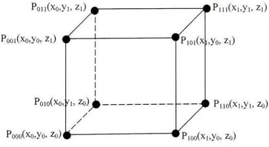
Trilinearinterpolationconsistsoftwosteps:theextraction _stepandtheinterpolation step.

In theextraction_{step, the} sub-cubeinthe source color spacethatcontains theinput point

is determined

by

a series of comparisons. The eight vertices ofthis cube are the lattice

points inthe source space, as shownin Figure 5.

Pon(xo,yi, zO

Pooi(xo!yo,z0

Poio(xo,Vi,_ZoLfc

Pooo(xOryo,Zo)

Pm(xi,yi,Zi)

y<>,zO

Pno(xi,yi,zo)

[image:32.499.103.365.396.539.2]

Pioo(xi>yo,Zq)

Figure 5: Sub-cubewithLattice Points DeterminedDuringExtraction

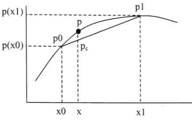
The interpolation _step consists of the repeated use of one-dimensional linear

Referring

to Figure

6,

a point_p on the curve between lattice points_po andpi is to be

interpolated.

[image:33.499.136.332.98.222.2]

xO x

Figure 6: ID Linear Interpolation

The interpolated value, pc(x), is

linearly

proportional to the ratio (x-xo)/(xi-xo).

Therefore,

Pc(x)=

P(X0)+

[p{*i)

-P{*o)]

Oi-*o)

Three-dimensional trilinear interpolation consists of seven linear interpolations on the

sub-cubedepictedin Figure 5. Thisresultsinthe

following

equations [5]:

Ax =_x

-xo

Ay=y-y0

Az= z-zo Co =Pooo ci =

(pioo

-pooo)/

(xi

-x0)

C2 =

(poio

-pooo)/

(yi

-yo)

C3 =

(P001

-POOO)/

(Zl

-Zo)

c4=

(pi

io-poio -pioo +Pooo)/

[(xi

-x0)

(yi

-yo)]

C5 =

(Pioi

-pooi-Pioo

+P000)

/

i(xi

-xo)

(z\-zo)]

C6 =

(pon

-Pool -Poio+P000) /

[(yi

-yo)

(zi-z0)]

cj=

(pm

-pon -pioi -pi10 +Pioo +Pooi +

Poio-Pooo)/

[(xi

-x0)

(yi

-yo)

(zi

-z0)]

p(x,y,z) =c0 +cjAx +_c2Ay +c3Az +c4AxAy +

5

Software

Implementation

Softwareprograms

implementing

the

Shepards, Moving

Matrix,

and ICIalgorithms were

written inthe _{C programming} language. Theprograms readdata files that contained the

forward printer _map and the gamut-mapped input points of the inverse map. The

programs executedthe algorithms onthis datato computetheinverse forthe giveninput

points; this output datawas written to separate data files for lateranalysis. The forward

printer _map was represented

by

two data files: one had 133

CMY _entries, and the other

had the _{corresponding} 133 LAB entries. This experimental printer data was obtained

from Dr. L. K. Mestha from Xerox.

5. 1

Algorithm Metrics

These software implementations and simulations provided relative accuracy, execution

time, andcomputational_complexityinformation foreach algorithm.

5.1.1

Determining

Algorithm

Complexity

The _complexity ofthe algorithms was measured objectively

by

including

code to count

the number ofmultiplication/division and square root operations performed to compute

the inverse. These operations are _costly in hardware because the modules to perform

themareboth large and slow ascomparedtoother operations. The algorithms were also

arithmetic _modules, the amount of parallelism that might be _exploited, and the

complexityofthe required control logic. A combination ofthe objective and subjective

complexitywas usedto rate each algorithm's overall_complexityrelativeto the others.

5.1.2

Determining

Algorithm

Execution Speed

The csh command interpreter_running ontheUnix platformhas abuilt-in utilitythat can

be used to determine the amount oftime a program is executing on the system. The

executiontimes ofthe programs were measured_{usingthis utility,} whichis an executable

named time. In order to form a valid _comparison, the programs were executed on the

same machineunderthe same environment. Program developmentand executionwas on

Rochester Institute ofTechnology's Grace computing system. Grace is an Alpha 4100

5/533 with3 EV5.6 CPUs. It has 1.5GB of_memoryandis running Tru64

UNIX,

version

4.0F.

5.1.3

Determining

Algorithm

Accuracy

The programs computed the inverse forthe 133

gamut-mapped LAB points x _using the

forward printer _{map data.} The completion of the programs resulted in a data file

containing

133

CMYentriesthatdefinedthe_{inverse y}:

y =

Eachpoint

5>;

was

interpolated

throughthe forwardprinter_{map P}to findthe_resultingzj.

The differences

AEj

_{between zy} and the _{corresponding xj} such that jk=

F'(xj)

were

computed. Thiscanbeshown_graphicallyas:

"j

*,.

>yj

>ZJ

AEj

'

Themean error and standard

deviation,

theminimumerror, andthemaximum error were

calculated from the

AEj

-these statistics representedthe _accuracyofthe algorithms. It

should be noted that these error statistics were computed _using the node points ofthe

inverse map as inputs. The accuracymetrics of each algorithmwere usedto comparethe

algorithms in terms of accuracy. Separate programs were written to perform the

interpolationthroughP and to compute the _accuracymetrics; these are also included on

the_{CD accompanying}thispaper.

5.2

Optimal Parameters

Each algorithm was executed several times while _varying the algorithm parameters.

Accuracy

metrics for each trial were measured to gain insight into how the parameters

affectthe accuracy. Thesetrials also ledto the values oftheparametersthatresultinthe

best accuracy. Tables _{showing the accuracy}data for differentparametervalues foreach

algorithm are shown in the Appendix (see Section 9.1). The results ofthese trials are

5.2.1

Shepard's Algorithm

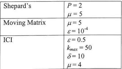
ForShepard's algorithm, there arethetwo variableparameters/* andju. The/?parameter

specifies how the distances between points are calculated. The trials showed that the

value of_p does not have much affect on the accuracy.

Therefore,

_p = ₂

was taken

because this isthemostconvenient as itresults inadistance measurementthat is_simply

the Euclidean distance. The /j. parameter affects the

locality

ofthe _{weighting function.}

The simulation results showthatju=₅

providesthebestaccuracy.

5.2.2

Moving

Matrix Algorithm

The variableparameters inthe

Moving

Matrix algorithm arejuand e. Similarto thesame

parameter in Shepard's _{algorithm, the} // parameter affects the

locality

ofthe regression.

Simulations showed that ju= ₅

resulted in thebest accuracy. The eparameter does not

have a significant affect on the _accuracy and is taken as a small value to avoid

ill-conditioningofthe

Si

matrix. Inthese simulations, fwastakenas

10" .

5.2.3 ICI Algorithm

The ICI algorithm has parameters _e,

kmaXt

5,

and /j.. s and

kmax

are the _{stop criteria;} s

specifies the error threshold at which the update iterations can _stop, and

kmax

is the

maximum number ofiterations that algorithm will perform when _computing the inverse

for a given point. Theparameter 8 for this algorithm specifies the perturbation used in

fu should be selected in order to achieve fast convergence and to meet _accuracy

requirements.

The software simulations showedthat themean errorforthisalgorithm canbereduced

by

decreasedthe errorthreshold s. Inorderto achieve _{fast convergence,} swastakenas0.5.

This is belowthe"justnoticeabledifference"ofAE= _{1.0. Other}

simulationshave shown

that even _{better accuracy} can be obtained

by

further _reducing s [4]. The software

simulations also showed that the best choice of

kmax

is 50.

Increasing

this parameter

beyond 50 does not result in substantial gains in _accuracy; ifthe algorithm is going to

converge for a given input _point, it will do so within 50 iterations. The perturbation 5

was determined to not _{have any} measurable affect on the _accuracy of_{the algorithm;} 5

was taken to be

10,

which is approximately a 4% variance ofthe printer's input color

components

(

0<

C, M,

Y<₂₅₅ and

10/255=0.04)

andis more orless arbitrary.

Finally,

thesimulations showed/j.=_4tobe

[image:38.499.135.347.553.673.2]

a good choiceintermsof_accuracyand convergence.

Table 1 showstheoptimal parameters foundforeach algorithm.

Table 1: Optimal Algorithm Parameters

Shepard's P=₂

/j= ₅

Moving

Matrix

=10"4

ICI 5=0.5

5=10

5.3

Simulation

Results

Theaccuracy, speed, and_complexityofeach algorithmis summarizedin Tables

2, 3,

and

4,

respectively. The metrics are obtained from the simulations _using optimal algorithm

parameters and _operating on the same data and on the same machine in the same

environment. All measurements are made forthe algorithms _computing the 133 inverse

map fromthe

133

[image:39.499.79.419.250.326.2]

forwardmap.

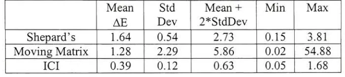
Table 2: Algorithm_Accuracy

Mean

AE

Std

Dev

Mean+

2*StdDev

Min Max

Shepard's 1.64 0.54 2.73 0.15 3.81

Moving

Matrix 1.28 2.29 5.86 0.02 54.88

ICI 0.39 0.12 0.63 0.05 1.68

Table 3: Algorithm Execution Time

ExecutionTime

(sec)

Shepard's 12

Moving

Matrix 17

ICI 7

Table4: Algorithm_Complexity

Shepard's LOW

Moving

Matrix HIGH

ICI MEDIUM

ICIis_clearlythe winnerinterms of_accuracyand execution speed. Abrief discussion of

each algorithm's_complexityfollows.

Moving

Matrix has significantlymore multiplications than Shepard's and _{approximately}

slow design.

Moving

Matrixalso would require complex control logictoperform matrix

operations such as matrixinversion.

Shepard's algorithm would be quite _easy to implement because it requires a small

number ofresources and is data flow oriented thus _{requiring very little} control logic.

However,

therearealargenumber of multiplications(threetimes thatof

ICI),

which will

result in a slow design. Even if more resources were used to perform some ofthe

processing inparallel (whichwouldincrease the design area), it is still _{unlikely it}would

beatout ICIinterms of speed. _{Although easy}to

implement,

Shepard's is inaccurateand

would most

likely

be slowerin hardwarethanICI.

ICI has the smallest number of _{multiplications,} which could result in a less complex

circuit.

However,

ICI has two significant drawbacks.

First,

this algorithm requires

trilinear

interpolation,

whichitselfisa non-trivialhardware implementation.

Second,

ICI

will require control logic for computing thegradientmatrix and for computingtheinitial

estimate

by

the_clusteringtechnique.

Of the three algorithms, ICI is the best in terms of speed, accuracy, and hardware

complexity. This algorithm was chosen for hardware implementation in VHDL. The

6

ICI

Hardware

Implementation

NOTE: All source VHDL files are located on the _{accompanying CD} under the

"Hardware/VHDL Source Code"

folder. The area and

timing

reports for each

sub-module described in this section can also be found on the _{accompanying CD} under the

"Hardware/Reports"

folder. VHDL source code is also shown in the Appendix (see

Section 9.2).

6. 1

Design

Methodology

The algorithm was implemented _{using VHDL.} The design was simulated with Mentor

Graphic's

ModelSim;

the simulation results were compared with results obtained from

software models _operating on the same input data. Correct

functionality

ofthe design

was guaranteed since the hardware simulation results matched those of the software

models.

The hardware modules were synthesized _{using Synopsys's Design Compiler} and was

targeted to a generic

library

providedwith the Synopsys'stools. _{The resulting}synthesis

resultsprovideanet-listthatcanbeusedfor ASIC fabrication.

Several important design decisions were made about the system _partitioning and

architecture, data storage, and datarepresentation. These decisions will be described in

6.1.1

System

Partitioning

and

Architecture

The ICI algorithm makes extensive use oftrilinearinterpolation. Trilinear interpolation

is a geometric method to calculate the output of a 3D function at a given input point,

where the 3D function is defined

by

a finite set ofinput and output pairs. A detailed

discussion oftrilinear

interpolation

can be found in Section 4.1.4. _{An entirely} separate

module was designed to perform trilinear

interpolation;

this module is used

by

the ICI

design and can alsobeusedinother applications.

Both the trilinear interpolation module and ICI module were designed using datapath

blocks and control blocks. This approach allows for

highly

controlled use of the

arithmetic units that make _up the datapaths. The advantage of

having

such control over

these units is that operations can be pipelined and the units can be shared where

appropriate.

6.1.2 Datastorage

Therearesix valuesfor each_{entry in}theforwardprinter_map

P;

oneforeach oftheinput

space components andone foreach ofthe output space components. For example, ifthe

P defines a_mapping from CMY to

LAB,

then there is a value for

C, M,

and Y for the

inputcolor _space, and avalue for

L, A,

andB forthe output colorspace. An

N3

look-up

table requires

6N3

bytes of storage. For

N=13,

this results in 13,182 bytes of required

Synthesis tools are still

incredibly

inefficient

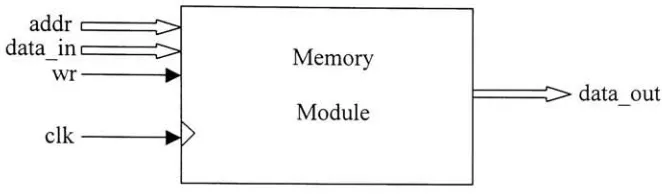
at _{synthesizing memory; therefore,} this

design assumes that an external _memory module exists that contains P. The memory

module in Figure 7 is assumed for designpurposes. The interpolation and ICI modules

aredesignedtointerfacewiththis_memorymodule.

[image:43.499.89.420.173.270.2]

C>data out

Figure 7:

Memory

Module Diagram

6.1.2.1 Operation

The memory module is synchronous and clocked

by

the elkinput _signal; all reads and

writes occur onthe _risingedge of elk and completeinone clock cycle. The operation of

themoduleisdescribed below.

(a)

Read: Readsoccur when wris

low;

data_outbecomesthevalue stored atthe

locationspecified

by

addr.

(b)

Write: Writes occur when wris

high;

thelocationspecified

by

addrisstored

(c) Memory

location: addr specifies the _{memory location} to read from

during

reads and the location to write to

during

writes. Its value can range from zero to

6N3-1.

The

interpolation

and ICImodulesthat

interface

to this_memorynever writeto

it;

thewr

and data_in signals are

included

forcompleteness.

6.1.2.2

Memory

Data Layout

It is assumed that the_memory module contains the fowardprinter

look-up

tableprior to

using the

functionality

oftheinterpolation and ICI modules.

Furthermore,

it is assumed

that thevalues are arrangedinthe_memorymoduleinthe

following

fashion:

Memory

Location Contents

0

Co

1

M0

2

Y0

3

Lo

4

A0

5

B0

6

Ci

7

Mi

8

Y,

9

Li

10

A,

6.1.3

Data Representation

The project specification requiredthat twodecimal places of_{accuracy be}retainedforthe

LAB values. This meant that the design would have to implement

floating

point

operations.

Floating

point_{hardware is}more complex and slowercomparedto fixedpoint

hardware.

Additionally,

the design resources did not have floating-point libraries that

containpre-compiled and optimizedfloating-pointmodules. These librarieswould either

have to be purchased, or a significant amount oftime and effort would be required to

designcustomfloating-pointarithmetic modules.

An alternative is to use fixed point arithmetic and scale all ofthe data to integers. The

approach allows for the use ofpre-compiled and optimized fixed point integer_modules,

whichsimplifiesthedesignand reduces designtime.

To preserve two decimal _{places, the} data had to be scaled

by

a factor of 100. For

example, 123.45 would be scaled as 123.45*100 = _{12345. Integer}

addition and

subtraction would occur normally.

However,

multiplications would require theresultto

bescaleddown. Thiscanbeshown

by

the

following

equations:

Original Operation: A* _B=_AB

With Scaled Data:

(

1 00

A)

*

(

1

00B)

= _{1 0000AB}

However,

we _onlywant

100AB,

which meansthisresultmustbe scaleddown

by

afactor

scaled fixed point _{arithmetic; multiplication operations must be followed}

by

division.

This disadvantage is a fair trade-off compared to the _complexity involved in

implementing

adesigntosupport

floating-point

numbers.

Itwas_necessaryto determine if_usingthis

integer-based

approach would compromisethe

accuracyofthe ICI algorithm. The ICI C language implementation files weremodified

touse _onlyinteger datainordertoinvestigatetheissue. The integerbased ICI Ccode is

located on the _accompanying CD under the "Software/integer-based ICI"

folder.

Simulation results showed that the _accuracy of the integer-based implementation was

equalto its

floating-point-based

counterpart.

6.2

Synthesis

Methodology

The control blocks of the trilinear interpolation and ICI modules are the _only

synchronous

(clocked)

blocks ineach ofthe designs. Theseblocks weresynthesized for

speed, and the maximum path

delay

through them defined the clock and maximum

operating

frequency

for the entire design. All otherblocks are _{asynchronous,} and their

maximum path delays are either shorter or longer than the defined clocked. For those

blocks that have a shorter maximum path

delay,

there is no concern because the circuit

will provide valid results within the clock period. For those blocks that have a longer

maximum path

delay,

thecontrolblocksmust either wait theappropriate amount of clock

cycles for the resultsto become valid or continueon with processing. In the latter case,

computation inthe block would continue as the control block would proceed with other

the logic flow. This concept of parallel computation motivated the design of several

separate datapaths that perform _{different functions. Wherever this type} ofparallelism

could not be _{exploited, the} control block _simply waits the appropriate amount ofclock

cycles forvaliddata.

There were no _{design specifications,} such as area or _speed, provided

by

the project

requirements for the hardware implementation.

However,

the design has application in

real-time and near real-time applications. Itwas also designed for ASIC implementation

inmind. For _{these reasons, the} designblocks were synthesized forthe fastest possible

performance. This is a reasonable synthesis constraint since the goal is real-time

computation, and the ASIC platform allows for larger and more complex designs as

comparedtoprogrammable

logic,

such as fieldprogrammable gate arrays(FPGA).

Theasynchronousblockswere constrained

by

_{specifying input}and outputdelays equalto

the defined clock. These constraints forced the synthesis tool to generate the fastest

possible

design,

but one that would never meet the

timing

constraints because ofthe

complexityofthe operations

being

performed. Several ofthe synthesizedblocks'

timing

reports _clearlyshowthat

they

donot meet

timing

constraints. This is acceptablebecause

inthis designmethodologyit is understoodthat theseblocks requiremorethanone clock

6.3

Simulation &

Testing

The VHDL code was simulated _{using Mentor} Graphic's ModelSim tool. Testbenches

were written in order to test and _verify correct

functionality

of the hardware design.

These testbenches read input data from

files,

_{fed it}to the module under _test, and wrote

the output data into another data file. Other inputs were also controlled

by

the

testbenches;

these

inputs,

such as algorithm _parameters, were the same as those used in

the C language software simulations. The output data files written

by

the testbenches

were compared to the output data files written

by

the C software models. Correct

functionality

of the VHDL design was guaranteed because the data contained in the

output files matched. The VHDL source code for the testbenches can be found in the

6.4

Hardware Modules

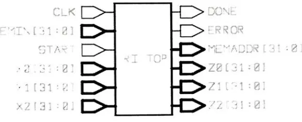
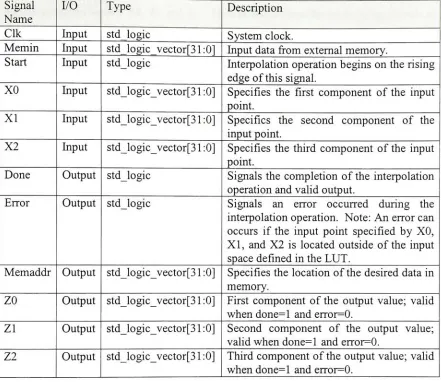
[image:49.499.99.410.223.349.2]

6.4.1 Trilinear Interpolation Module

(trijop.vhd)

Figure 8 shows the I/O signals ofthe trilinear interpolationmodule, andFigure 9 shows

theblock diagram ofthemodule. Inputand outputsignals aredescribed in Table 5.

I -8

O **t

5fAR'f

'H3t'8

O-"<? i.,erst.

r ADS?

-O

a;.

c

-f**>2atj: as

-Ozra: 2

.TERfc.

[image:50.499.48.450.32.657.2]

Table5:Trilinear InterpolationModule I/O Signals

Signal

Name

I/O Type Description

Clk Input stdlogic Systemclock.

Memin Input std_logic _{vector[31:0] Input datafrom}externalmemory.

Start Input std_logic Interpolation operationbeginsonthe

rising

edge ofthissignal.

XO Input std_logic_vector[3_{1 :0]} Specifies the first component of the input

point.

XI Input std_logic_vector[3_{1 :0]} Specifics the second component of the

inputpoint.

X2 Input std_logic_vector[3_{1 :0]} Specifies the third component ofthe input

point.

Done Output stdlogic Signals the completion ofthe interpolation

operation andvalidoutput.

Error Output std_logic Signals an error occurred

during

the

interpolationoperation. Note: Anerror can

occurs ifthe input point specified

by

XO,

XI,

and X2 is located outside ofthe input

spacedefined intheLUT.

Memaddr Output std_logic_vector[3_{1 :0]} Specifiesthelocationofthedesired data in

memory.

ZO Output std_logic_vector[3_{1 :0]} First component ofthe output _value; valid

whendone=l and error=0.

Zl Output std_logic_vector[31_:0] Second component of the output _value;

valid whendone=l and error=0.

Z2 Output std_logic_vector[31_:0] Thirdcomponent oftheoutput _value; valid

whendone=l and error=0.

6.4.1.1

Operation

The system clockmusthave aperiod of40nanoseconds or_{greater; this} correspondsto a

maximum _operating

frequency

of25 MHz. Simulationresults show that this design can [image:51.499.28.469.85.467.2]

The

rising

edge of startbegins

interpolation

attheinputpoint specified

by

signals

XO,

XI

and X2. Done is asserted when

interpolation

_is complete. Iferror is not _raised, valid

output occurs on signals

ZO,

Zl and Z2. Memin and memaddr are interface signals to

the external _memorymodule. _{Memin is data comingfromthe memory;} memaddris the

location in _memory of desired data and is controlled

by

the interpolation module's

controlblock.

6.4.1.2

Sub-blocks

6.4.1.2.1

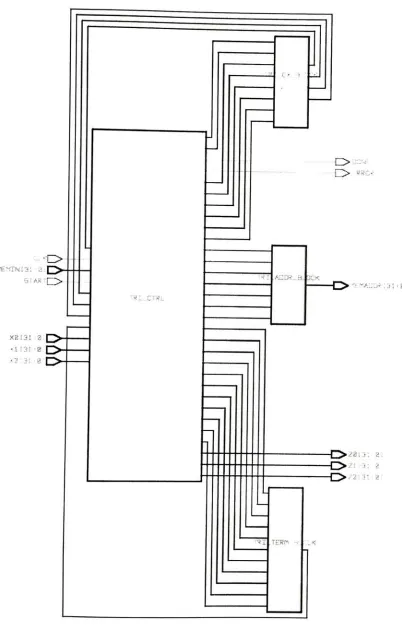
TRI_CTRL_BLOCK

(trictrl.vhd)

This blockcontains the control logic neededto _carryout the interpolation. Its input and

output signals interface to the other sub-blocks and to the external _memory module to

control data flow. It is also responsible for

beginning

the interpolation when start is

raisedandfor asserting done and errorwhentheinterpolation is complete.

The

top

level diagram is shown in Figure 10. A lower level block diagram is not

available because it contains too _{many low-level} components

(primarily

_registers) and

ADDl.^KS.uLTtj'.*21 c^O-fCHlNI3iai

sta*-

rj>-SUB1.RESULT131_i!3 SuB2.,.RE5Ui.7i3la

?>jy:i..RESULT'3! JZ|

T. *E.SU-7t3!81 x*r3!;?i x.H3l>81 X2C21:8. OADDlAt:ji .a) OAHJ1Bl3l=ai -ODO -t>&SOS? 4J*^Su8lAt31tai OsuBib;^: 31 -^:>wH2A;21 -21 Os-^;'::i:-*8J f3>s.u:i:tA:a: a;

^g^P*&Jl&4:' . '&>.

f^T*I-MXnJB>-334l(31 z: HD^'^i A.j.^ ;>>_BC!3l:SI

OtI.A0aR_SP_IN3131>B!

PTgi-ADaa jy-m!3i-0! PTg X-AICT JP 3>ft131Bi

O"^X-ADOR-DP.JCNB1 31m

"OTKI..ADLK_0>*_I>i/*3i m ">Uli3! <|]

O

"--CJI3I:J -5*T_C2:31'81

4S>T-X35 3!:ii!;

<0*..r^!31'Bi

f^1"-CSi3i-a.

4Q>Tj:8f3t

k-|">T.X?!3! :2;

f^"..;;xf3l ;!

f^TJjriSI =81

>0"_D2t3I^l

-0/;i3t <bi

[image:53.499.70.430.42.435.2]

0/tni:^. n -gi

Figure 10:

Top

Level DiagramofTrilinear Interpolation TRI CTRLBlock

The area ofthisblock is 18,148 cells. The maximum path

delay

through this block is

6.4.1.2.2

TRI

ADDR BLOCK

(triaddrblock.vhd)

This block defines the datapath for_calculating the_memory address of adesiredvalue in

memory. The dataneeded from_memory arethe lattice points ofthe cell _{containing the}

inputpoint andtheir_{corresponding}pointsinthe output. These latticepoints are located

by

indices which were determined

by

_searching the input space forthe appropriate cell

containing the input point. These indices are input to this block which computes the

memoryaddressofthedesiredvalues.

The

top

_{level diagram showing input} and output signals ofthis block can be found in

Figure 1 1. Alowlevel block diagramisshownin Figure 12.

INZt3l"81

D*-!N3!3I'0)

O-33N5131-81 O"

1NBI3I :'B'CJ>"

"C^r 131-01

T'" *>

[image:54.499.141.362.329.480.2]

[image:55.499.40.459.35.404.2]

Figure 12: Datapath ArchitectureofTRI ADDRJBLOCK

The area ofthis block is 20,014 cells. The maximum path

delay

through this block is

38.87nanoseconds.

6.4.1.2.3 TRI CX

BLOCK

(tri_cx_block.vhd)

This block defines the datapath for calculating the CI through C7 values (henceforth

knownas CX values) usedto calculate the output. These values are calculatedfromthe

isneededto compute all seven valuesbecausethese units are shareddueto_pipeliningof

operations

by

thecontrolblock.

The

top

_{level diagram showing input and output signals ofthis block} can be found in

Figure 13. Alow level block

diagram

isshownin Figure 14.

Ar;31A[31-'B3

a::::ibi2: -ei

f^>-5l.;B1Ani:g)

SUB2A[3! <gj

sugzB'3* -b'i

&J33AI'J 1 :_ii

St63Bl3t s^J

A:.:-Dl_??rSULTl31rgI

5u3! ??fcSJLTtjt=81

SUB2_RESULT{31 ^81

-OstS3_SESULTt31-2!

[image:56.499.117.380.206.343.2]

TI_CX_3_

[image:56.499.36.461.421.631.2]

Figure 13:

Top

Level DiagramofTrilinear Interpolation TRI CX BLOCK

The area ofthis block is 3,658 cells. The maximum path

delay

through this block is

10.36nanoseconds.

6.4.1.2.4 TRI TERM BLOCK

(tritermblock.vhd)

Thisblockdefinesthe datapath_{for calculating}theinterpolated_values; it istheworkhorse

ofthe interpolation module. It uses the CX values produced

by

the TRICXBLOCK

and several otherinputsprovided

by

thecontrolblocktocomputetheinterpolatedvalues.

The

top

level diagram _showing input and output signals ofthis block can be found in

Figure 15. A low level block diagram isshowninFigure 16. Thedisadvantageof_using

scaleddata canbe seen in this low level

diagram;

there are divide units throughout the

datapath that are needed to scale down theresults ofthe multiplication-rich calculation

performed

by

this block. These divides units add significant area and delays to th