Toward efficacy of piecewise polynomial truncated singular value decomposition algorithm in moving force identification

1

Toward efficacy of piecewise polynomial truncated singular value decomposition

algorithm in moving force identification

Zhen Chen

_{, Lifeng Qin}

_{, Shunbo Zhao}

_{, Tommy H.T. Chan}

_{, Andy Nguyen}

a

International Joint Research Lab for Eco-building Materials and Engineering of Henan, North China University of Water Resources and Electric Power, Zhengzhou 450045, China

b _{School of Civil Engineering and Built Environment, Queensland University of Technology (QUT), Brisbane, 4000,}

Australia

c _{School of Civil Engineering of Surveying, University of Southern Queensland (USQ), Springfield Central, 4300,}

Australia

Abstract: This paper introduces and evaluates the piecewise polynomial truncated singular value decomposition (PP-TSVD) algorithm toward an effective use for moving force identification (MFI). Suffering from numerical

non-uniqueness and noise disturbance, the MFI is known to be associated with ill-posedness. An important method for

solving this problem is the truncated singular value decomposition (TSVD) algorithm but the truncated small singular

values removed by TSVD may contain some useful information. The PP-TSVD algorithm extracts the useful

responses from truncated small singular values and superposes it into the solution of TSVD, which can be useful in

MFI. In this paper, a comprehensive numerical simulation is set up to evaluate PP-TSVD, and compare this technique

against TSVD and SVD. Numerically simulated data are processed to validate the novel method, which show that

regularization matrix 𝐋𝐋 and truncating point 𝑘𝑘 are two most important governing factors affecting identification

accuracy and ill-posedness immunity of PP-TSVD.

Keywords: moving force identification, piecewise polynomial truncated singular value decomposition, ill-posedness, regularization matrix, truncating point

1 Introduction

The identification of moving forces acting on bridges is an important practical problem in structural dynamics, for

instance, to guide the design of bridges as live load components in the bridge design code. Although the forward

model of load identification has been established, most of the identification methods involve in singular value

decomposition (SVD) in the identification process. In addition, the small singulars of the system matrix decide the

great degree of system ill-posedness and lead to a large identified error (Liu et al., 2017). In the past, there has been significant research effort to solve this problem by Chan et al. (2001, 2006).

Comparative studies (Yu and Chan, 2007) show that the time domain method (TDM) (Law et al., 1997) and

frequency-time domain method (FTDM) (Law et al., 1999) are clearly better than those from both interpretive method

I (IMI) (O’Connor and Chan, 1998) and interpretive method II (IMII) (Chan et al., 1999). The inverse problems

involving dynamic parameter identification in time domain or frequency-time domain have been studied by many

researchers (Zhu and Law, 2006; Zhu et al., 2018). However, due to matrix ill-posedness and noise disturbance in

moving force identification (MFI), the identification accuracy of many methods is still not high enough since the

nature of the inverse problem is ill-posed (Yu et al., 2016).

The Tikhonov regularization approach is very effective with ill-posed problems due to matrix ill-posedness and

noise disturbance (Busby and Trujillo, 1997). Choi et al. (2007) indicated that the reconstructed forces can be

improved by choosing the optimal regularization parameter of Tikhonov regularization. Ding et al. (2015) presented

unscented Kalman filter technique to identify the structural parameters and coefficients of the orthogonal

decomposition. Ronasi et al. (2011) adopted the traditional Tikhonov regularization as a means to further reduce the

impact of noise on choosing the suitable resolution for the sought load. Lu and Liu (2011) proposed a dynamic

*_{Corresponding author.}

2

response sensitivity-based finite element model updating approach to identify both the vehicular parameters and the

structural damages. Li et al. (2013) presented an adaptive Tikhonov regularization technique to improve the damage

identification results when noise effect is included. Liu et al. (2015) adopted an improved regularization to overcome

the ill-posedness of load reconstruction by selecting the filter function. Besides Tikhonov regularization, there are

many other optimization methods with properties that make them better suited to certain problems to combat the

ill-posedness (Sanchez and Benaroya, 2014).

Recent years have witnessed many new approaches adopted for solving the MFI problem such as updated static

component technique (Pinkaew, 2006), cross entropy optimization approach (Dowling et al., 2012), Bayesian

inference regularization (Feng et al., 2015), truncated generalized singular value decomposition algorithm (Chen and

Chan, 2017), modified preconditioned conjugate gradient method (Chen et al., 2018) and weighted l1-norm

regularization method (Pan et al., 2018). The SVD technique is much better than direct pseudo-inverse solution for

MFI with TDM but the identification accuracy is still sensitive to perturbations. The truncated singular value

decomposition (TSVD) technique has been widely used in discrete linear ill-posed problems, which provides

significant improvements to the least-squares estimator to derive a single optimal solution for a given problem (Xu,

1998; Bouhamidi et al., 2011). The TSVD uses only the largest singular values to derive the solution and small singular values are more or less arbitrarily discarded. By truncating the small singular values, TSVD can effectively

filter the noise component in measurement responses but the truncating process inevitably discards some true

responses including in small singular values. Studies by Winkler (1997a, 1997b) indicated that an important aspect in

using TSVD is the deletion of the correct number of singular values of the coefficient matrix and polynomial basis

conversion can be used to improve this problem.

Hansen and Mosegaard (1996) presented a piecewise polynomial truncated singular value decomposition

(PP-TSVD) approach but the choosing of the optimal parameter has not been proposed. The PP-TSVD algorithm extracts

the true responses from truncated small singular values and superposes it into the solution of TSVD, which offset the

disadvantage of TSVD perfectly. Giustolisi (2003) indicated that the PP-TSVD can overcome poor generalization

properties due to the high dimensionality and non-Gaussian noise. Sobouti et al. (2016) adopted the PP-TSVD to solve

the total variation regularized inverse problem. However, there has been a lack of study on evaluation of the PP-TSVD

and absent rules for choosing the optimal parameter of the PP-TSVD.

As mentioned above, the PP-TSVD method is very effective in solving the linearized ill-posed problems, which has

excellent theoretical completeness and offset the disadvantage of TSVD perfectly. In this paper, a comprehensive

numerical simulation survey is set up to compare this algorithm against TSVD and SVD. Furthermore, the governing

regularization parameters of the PP-TSVD have been scrutiny selected, such as the regularization matrix 𝐋𝐋 and the

truncating point 𝑘𝑘. The numerical results show that the PP-TSVD has significant improvement compared with TSVD

and TDM, which has important theoretical and provide a useful approach for the MFI.

2 Theory of moving force identification

2.1. Theory of time domain method (TDM)

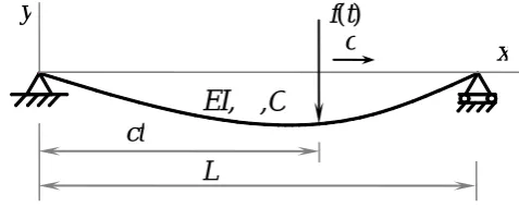
As shown in Fig. 1, assuming the bridge is of constant cross-section with constant mass per unit length 𝜌𝜌, having

linear, viscous proportional damping 𝐶𝐶 and with span length𝐿𝐿, Young’s modulus 𝐸𝐸 and second moment of inertia of

the beam cross-section 𝐼𝐼, neglecting the effects of shear deformation and rotary inertia, and with the force 𝑓𝑓(𝑡𝑡)

moving from left to right at a prescribed velocity 𝑐𝑐 at time 𝑡𝑡, the equation of motion in terms of the modal coordinate

𝑞𝑞𝑛𝑛(𝑡𝑡)can be written as

3

where𝑝𝑝_𝑛𝑛(𝑡𝑡) =𝑓𝑓(𝑡𝑡) sin𝑛𝑛𝑛𝑛𝑛𝑛𝑛𝑛

𝜌𝜌 is the modal force; 𝜔𝜔𝑛𝑛= 𝑛𝑛2_𝑛𝑛2

𝜌𝜌2 � 𝐸𝐸𝐸𝐸

𝜌𝜌 is the n-th modal frequency; 𝜉𝜉𝑛𝑛= 𝐶𝐶

2𝜌𝜌𝜔𝜔𝑛𝑛 is the modal

damping ratio.

f(t)

EI,

ρ

,C

c

y

x

L

ct

Fig. 1. Model of moving force identification

Equation (1) can be solved in the time domain by the convolution integral, yielding

𝑞𝑞𝑛𝑛(𝑡𝑡) =_{𝜌𝜌𝜌𝜌}2 ∫ ℎ₀𝑛𝑛 𝑛𝑛(𝑡𝑡 − 𝜏𝜏)𝑝𝑝(𝜏𝜏)𝑑𝑑𝜏𝜏 (2)

where ℎ_𝑛𝑛(𝑡𝑡) =_𝜔𝜔1

𝑛𝑛

′ 𝑒𝑒−𝜉𝜉𝑛𝑛𝜔𝜔𝑛𝑛𝑛𝑛sin(𝜔𝜔𝑛𝑛′𝑡𝑡)and 𝜔𝜔𝑛𝑛′ =𝜔𝜔𝑛𝑛�1− 𝜉𝜉𝑛𝑛2.

At point 𝑥𝑥 and time 𝑡𝑡, the deflection 𝐯𝐯(𝑥𝑥,𝑡𝑡) of the simply supported beam can be expressed as Law et al. (1997)

with modal superposition

𝐯𝐯(𝑥𝑥,𝑡𝑡) =�_{𝜌𝜌𝐿𝐿𝜔𝜔}2 𝑛𝑛′ ∞

𝑛𝑛=1

sin𝑛𝑛𝑛𝑛𝑥𝑥_𝐿𝐿 � 𝑒𝑒−𝜉𝜉𝑛𝑛𝜔𝜔𝑛𝑛(𝑛𝑛−𝜏𝜏)sin𝜔𝜔_𝑛𝑛′(𝑡𝑡 − 𝜏𝜏)sin𝑛𝑛𝑛𝑛𝑐𝑐𝜏𝜏

𝐿𝐿 𝑓𝑓(𝜏𝜏)d𝜏𝜏 𝑛𝑛

0

(3)

At point 𝑥𝑥 and time 𝑡𝑡, the bending moment 𝐌𝐌(𝑥𝑥,𝑡𝑡) of the simply supported beam can be expressed as

𝐌𝐌(𝑥𝑥,𝑡𝑡) =−𝐸𝐸𝐼𝐼𝜕𝜕2_{𝜕𝜕𝑥𝑥}𝜈𝜈(𝑥𝑥₂,𝑡𝑡)=�2𝐸𝐸𝐼𝐼𝑛𝑛_{𝜌𝜌𝐿𝐿3}2 ∞

𝑛𝑛=1

𝑛𝑛2 𝜔𝜔𝑛𝑛′sin

𝑛𝑛𝑛𝑛𝑥𝑥

𝐿𝐿 � 𝑒𝑒−𝜉𝜉𝑛𝑛𝜔𝜔𝑛𝑛(𝑛𝑛−𝜏𝜏)sin𝜔𝜔𝑛𝑛′(𝑡𝑡 − 𝜏𝜏)sin𝑛𝑛𝑛𝑛𝑐𝑐𝜏𝜏_{𝐿𝐿 𝑓𝑓}(𝜏𝜏)d𝜏𝜏 𝑛𝑛

0

(4)

Assuming that the time-varying force 𝑓𝑓(𝑡𝑡) is a step function about the time sampling interval ∆t, and then the

equation (4) can be rewritten in discrete terms as

𝑀𝑀(𝑖𝑖) =2𝐸𝐸𝐼𝐼𝑛𝑛_{𝜌𝜌𝐿𝐿3}2�𝑛𝑛2 𝜔𝜔𝑛𝑛′ 𝑠𝑠𝑖𝑖𝑛𝑛

𝑛𝑛𝑛𝑛𝑥𝑥

𝐿𝐿 � 𝑒𝑒−𝜉𝜉𝑛𝑛𝜔𝜔𝑛𝑛𝛥𝛥𝑛𝑛(𝑖𝑖−𝑗𝑗)𝑠𝑠𝑖𝑖𝑛𝑛 𝜔𝜔𝑛𝑛′ 𝛥𝛥𝑡𝑡(𝑖𝑖 − 𝑗𝑗)sin

𝑛𝑛𝑛𝑛𝑐𝑐∆𝑡𝑡𝑗𝑗

𝐿𝐿 𝑓𝑓(𝑗𝑗) 𝑖𝑖= (0, 1 , 2 , … , N) 𝑖𝑖

𝑗𝑗=0 ∞

𝑛𝑛=1

(5)

where N + 1 is the number of sample points. Let

𝐶𝐶𝑥𝑥𝑛𝑛=2𝐸𝐸𝐸𝐸𝑛𝑛 2 𝜌𝜌𝜌𝜌3

𝑛𝑛2 𝜔𝜔_𝑛𝑛′ 𝑠𝑠𝑖𝑖𝑛𝑛

𝑛𝑛𝑛𝑛𝑥𝑥

𝜌𝜌 𝛥𝛥𝑡𝑡 𝐸𝐸𝑛𝑛𝑖𝑖−𝑗𝑗 =𝑒𝑒−𝜉𝜉𝑛𝑛𝜔𝜔𝑛𝑛𝛥𝛥𝑛𝑛(𝑖𝑖−𝑗𝑗)

𝑆𝑆1(𝑖𝑖 − 𝑗𝑗) =𝑠𝑠𝑖𝑖𝑛𝑛 𝜔𝜔𝑛𝑛′ 𝛥𝛥𝑡𝑡(𝑖𝑖 − 𝑗𝑗) 𝑆𝑆2(𝑗𝑗) =𝑠𝑠𝑖𝑖𝑛𝑛(𝑛𝑛𝑛𝑛𝑛𝑛𝛥𝛥𝑛𝑛_𝜌𝜌 𝑗𝑗) (6)

Then the equation (5) can be arranged into matrix form as

⎩ ⎪ ⎨ ⎪ ⎧𝑀𝑀_𝑀𝑀(0)₍₁₎

𝑀𝑀(2)

⋮ 𝑀𝑀(𝑁𝑁)⎭⎪

⎬ ⎪ ⎫

=∑∞ 𝐶𝐶𝑛𝑛𝑥𝑥 𝑛𝑛=1 ×

⎣ ⎢ ⎢ ⎢

⎡0₀ 0₀ 0₀ ⋯_⋯ 0₀

0 𝐸𝐸𝑛𝑛1_{𝑆𝑆1(1)𝑆𝑆2(1) 0 ⋯ 0}

⋮ ⋮ ⋮ ⋱ ⋮

0 𝐸𝐸𝑛𝑛𝑁𝑁−1𝑆𝑆1(𝑁𝑁 −1)𝑆𝑆2(1) 𝐸𝐸𝑛𝑛𝑁𝑁−2𝑆𝑆1(𝑁𝑁 −2)𝑆𝑆2(2) ⋯ 𝐸𝐸𝑛𝑛𝑁𝑁−𝑁𝑁𝐵𝐵𝑆𝑆1(𝑁𝑁 − 𝑁𝑁𝐵𝐵)𝑆𝑆2(𝑁𝑁𝐵𝐵)⎦ ⎥ ⎥ ⎥ ⎤ × ⎩ ⎪ ⎨ ⎪ ⎧𝑓𝑓_𝑓𝑓(0)₍₁₎

𝑓𝑓(2)

⋮ 𝑓𝑓(𝑁𝑁𝐵𝐵)⎭⎪

⎬ ⎪ ⎫

(7)

where 𝑁𝑁_𝐵𝐵 = 𝜌𝜌

𝑛𝑛𝛥𝛥𝑛𝑛. The time-varying force 𝑓𝑓(𝑡𝑡) is equal to 0 when the vehicle just get on or off the bridge, that is，

𝑓𝑓(0) = 0 and 𝑓𝑓(𝑁𝑁_𝐵𝐵) = 0 which corresponding to 𝑀𝑀(0) = 0 and 𝑀𝑀(1) = 0. Then the equation (7) can be condensed as

� 𝑀𝑀(2)

𝑀𝑀(3)

⋮ 𝑀𝑀(𝑁𝑁)

�=∑∞𝑛𝑛=1𝐶𝐶𝑛𝑛𝑥𝑥×

⎣ ⎢ ⎢

⎡ 𝐸𝐸𝑛𝑛1𝑆𝑆1(1)𝑆𝑆2(1) 0 ⋯ 0

𝐸𝐸𝑛𝑛1𝑆𝑆1(2)𝑆𝑆2(1) 𝐸𝐸𝑛𝑛1𝑆𝑆1(1)𝑆𝑆2(2) ⋯ 0

⋮ ⋮ ⋱ 0

𝐸𝐸𝑛𝑛𝑁𝑁−1𝑆𝑆1(𝑁𝑁 −1)𝑆𝑆2(1) 𝐸𝐸𝑛𝑛𝑁𝑁−2𝑆𝑆1(𝑁𝑁 −2)𝑆𝑆2(2) ⋯ 𝐸𝐸𝑛𝑛𝑁𝑁−𝑁𝑁𝐵𝐵+1𝑆𝑆1(𝑁𝑁 − 𝑁𝑁𝐵𝐵+ 1)𝑆𝑆2(𝑁𝑁𝐵𝐵−1)⎦

⎥ ⎥ ⎤ ×� 𝑓𝑓(1) 𝑓𝑓(2) ⋮ 𝑓𝑓(𝑁𝑁𝐵𝐵−1)

� (8)

where 𝑀𝑀(𝑖𝑖) is the bending moment of the 𝑖𝑖-th sampling interval and 𝑓𝑓(𝑖𝑖) is the axle force of the 𝑖𝑖-th sampling

4

Equation (8) is simply rewritten as

𝐵𝐵

(𝑁𝑁−1)(𝑁𝑁𝐵𝐵−1)

⋅

𝑓𝑓

=

𝑀𝑀

Similarly, at point 𝑥𝑥 and time 𝑡𝑡, the acceleration 𝐯𝐯̈(𝑥𝑥,𝑡𝑡) of the simply supported beam can be expressed as

𝐯𝐯̈(𝑥𝑥,𝑡𝑡) =�_{𝜌𝜌𝐿𝐿}2 sin𝑛𝑛𝑛𝑛𝑥𝑥_𝐿𝐿

∞

𝑛𝑛=1

[𝑓𝑓(𝑡𝑡)sin𝑛𝑛𝑛𝑛𝑥𝑥_𝐿𝐿 +� ℎ̈𝑛𝑛(𝑡𝑡 − 𝜏𝜏)𝑓𝑓(𝜏𝜏)sin𝑛𝑛𝑛𝑛𝑐𝑐𝜏𝜏_𝐿𝐿 d𝜏𝜏] 𝑛𝑛

0

(10)

where ℎ̈_𝑛𝑛(𝑡𝑡) = 1 𝜔𝜔𝑛𝑛′ 𝑒𝑒

−𝜉𝜉𝑛𝑛𝜔𝜔𝑛𝑛𝑛𝑛× {[(𝜉𝜉_𝑛𝑛𝜔𝜔_𝑛𝑛)2− 𝜔𝜔_𝑛𝑛′2] sin𝜔𝜔_𝑛𝑛′𝑡𝑡+ (−2𝜉𝜉_𝑛𝑛𝜔𝜔_𝑛𝑛𝜔𝜔_𝑛𝑛′) cos𝜔𝜔_𝑛𝑛′𝑡𝑡}_.

Equation (10) can also be arranged into matrix form and simply rewritten as

𝑣𝑣̈

𝑁𝑁×1

=

𝐴𝐴

⋅

𝑓𝑓

(𝑁𝑁𝐵𝐵−1)×1

As shown above, the relationship between the time-varying force 𝑓𝑓(𝑡𝑡) and the bending moment responses or

acceleration responses can be rewritten in discrete terms and rearranged into a set of linear equations, which also can

be modified for the identification of multi-forces in terms of the linear superposition principle.

2.2 Theory of truncated singular value decomposition (TSVD)

The singular value decomposition of system matrix 𝐀𝐀 in MFI can be described as

𝐀𝐀=𝐔𝐔𝐔𝐔𝐕𝐕𝑇𝑇 _{=� 𝐮𝐮} 𝑖𝑖 𝑛𝑛

𝑖𝑖=1

𝛔𝛔𝑖𝑖𝐯𝐯𝑖𝑖𝑇𝑇

(12)

where 𝐔𝐔= (𝐮𝐮₁,𝐮𝐮₂,⋯ 𝐮𝐮_𝑛𝑛) and 𝐕𝐕= (𝐯𝐯₁,𝐯𝐯₂,⋯ 𝐯𝐯_𝑛𝑛) are orthonormal columns matrices with 𝐔𝐔𝑇𝑇𝐔𝐔=𝐕𝐕𝑇𝑇𝐕𝐕=𝐈𝐈_𝑛𝑛, 𝐮𝐮_𝑖𝑖𝐮𝐮_𝑖𝑖𝑇𝑇 = 1, 𝐯𝐯_𝑖𝑖𝐯𝐯_𝑖𝑖𝑇𝑇 = 1, ∑= diag(𝜎𝜎₁,𝜎𝜎₂,⋯,𝜎𝜎_𝑛𝑛) with 𝜎𝜎₁≥ 𝜎𝜎₂≥ ⋯ ≥ 𝜎𝜎_𝑛𝑛≥0. The first singular values of vehicle-bridge system matrix 𝐀𝐀 is 𝜎𝜎₁ and the 𝑛𝑛-th singular values of matrix 𝐀𝐀 is 𝜎𝜎_𝑛𝑛, then the condition number of system matrix 𝐀𝐀 is 𝜎𝜎1

𝜎𝜎𝑛𝑛.

With one or more very small singular values existing in system matrix, the condition number of system matrix 𝐀𝐀 is

very large relative to 𝜎𝜎₁ and then leading to ill-posedness of MFI. The best approach to reduce the abnormal large

condition number of 𝐀𝐀 is to truncate very small singular values by using TSVD.

The TSVD approach can be described as

𝐀𝐀𝑘𝑘 =𝐔𝐔𝐔𝐔𝐕𝐕𝑇𝑇 =� 𝐮𝐮𝑖𝑖 𝑘𝑘

𝑖𝑖=1

𝛔𝛔𝑖𝑖𝐯𝐯𝑖𝑖𝑇𝑇 𝑘𝑘 ≤ 𝑛𝑛

(13)

Then the solutions of vehicle-bridge system equation 𝐀𝐀𝐀𝐀=𝐛𝐛 with TSVD approach can be described as the

minimization problem

min‖𝐀𝐀‖2 subject to min‖𝐀𝐀𝑘𝑘𝐀𝐀 − 𝐛𝐛‖2 (14)

The solution of TSVD can be obtained as

𝐀𝐀𝑘𝑘 =𝐀𝐀𝑘𝑘−1𝐛𝐛=�∑𝑘𝑘𝑖𝑖=1𝐮𝐮𝑖𝑖𝛔𝛔𝑖𝑖𝐯𝐯𝑖𝑖𝑇𝑇�−1𝐛𝐛 𝑘𝑘 ≤ 𝑛𝑛 (15)

According to the property ofvectors 𝐮𝐮_𝑖𝑖 and 𝐯𝐯_𝑖𝑖, the TSVD solutions of 𝐀𝐀𝐀𝐀=𝐛𝐛 can be expressed as

𝐀𝐀𝑘𝑘=�𝐮𝐮𝑖𝑖 𝑇𝑇_𝐛𝐛

𝛔𝛔𝑖𝑖 𝐯𝐯𝑖𝑖 𝑘𝑘

𝑖𝑖=1

(16)

The 2-norm of 𝐀𝐀_𝑘𝑘satisfies ‖𝐀𝐀_𝑘𝑘‖2₂=∑𝑘𝑘_𝑖𝑖=1𝜎𝜎_𝑖𝑖−2�𝐮𝐮_𝑖𝑖𝑇𝑇𝐛𝐛�2, and thus ‖𝐀𝐀‖_𝟐𝟐 is increased with 𝑘𝑘. The truncating point 𝑘𝑘 is

an important regularization parameter of the TSVD, which controls the amount of stabilization imposed on 𝐀𝐀_𝑘𝑘 and the

5

still has some limitations such as the data over-fitting problem. Therefore, the PP-TSVD is presented to avoid data

over-fitting problem since some additional responses are extracted from truncated small singular values compared

with TSVD.

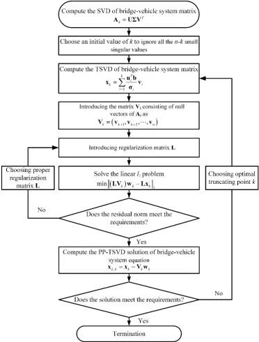
2.3 Theory of piecewise polynomial truncated singular value decomposition (PP-TSVD)

The regularization of ‖𝐀𝐀‖_𝟐𝟐is often more appropriate by minimizing the seminorm ‖𝐋𝐋𝐀𝐀‖_𝟐𝟐. 𝐋𝐋is the regularization

matrix which can be obtained from discrete approximation of derivative operators. Assuming that 𝐋𝐋 is �𝑛𝑛 −

(𝑝𝑝 −1)�×𝑛𝑛 and has full row rank, the 𝑝𝑝 −1 is less than truncating point 𝑘𝑘 corresponding to (𝑝𝑝 −1)-th derivative operator, in which the seminorm ‖𝐋𝐋𝐀𝐀‖_𝟐𝟐is introduced to replace the original linear system min‖𝐀𝐀‖_𝟐𝟐, i.e.,

min‖𝐋𝐋𝐀𝐀‖2 subject to min‖𝐀𝐀𝑘𝑘𝐀𝐀 − 𝐛𝐛‖2 (17)

By introducing the matrix 𝐕𝐕_𝑘𝑘 consisting of null vectors of 𝐀𝐀_𝑘𝑘 as

𝐕𝐕𝑘𝑘 = (𝐯𝐯𝑘𝑘+1,𝐯𝐯𝑘𝑘+2,⋯,𝐯𝐯𝑛𝑛) (18)

In order to extract some additional responses from truncated small singular values of TSVD, the solution 𝐀𝐀_L

consists oftheTSVD solution 𝐀𝐀_𝑘𝑘 plus a modification, which can be expressed as

𝐀𝐀L =𝐀𝐀𝑘𝑘− 𝐕𝐕𝑘𝑘(𝐋𝐋𝐕𝐕𝑘𝑘)+𝐋𝐋𝐀𝐀𝑘𝑘 (19)

where (𝐋𝐋𝐕𝐕_𝑘𝑘)+ is the pseudoinverse of 𝐋𝐋𝐕𝐕_𝑘𝑘. Form a computational point of view, the vector 𝐰𝐰_𝑘𝑘 = (𝐋𝐋𝐕𝐕_𝑘𝑘)+𝐋𝐋𝐀𝐀_𝑘𝑘 is simply the least squares solution to the problem min‖(𝐋𝐋𝐕𝐕_𝒌𝒌)𝐰𝐰_𝑘𝑘− 𝐋𝐋𝐀𝐀_𝑘𝑘‖₂.

The PP-TSVD algorithm is derived from equation (17) by replacing the 2-norm of 𝐋𝐋𝐀𝐀 with the 1-norm. Thus, the

solution of the above problem can be expressed as Hansen and Mosegaard (1996)

min‖𝐋𝐋𝐀𝐀‖1 subject to min‖𝐀𝐀𝑘𝑘𝐀𝐀 − 𝐛𝐛‖1 (20)

Then the solution of PP-TSVD 𝐀𝐀_L,𝑘𝑘 can be expressed as

𝐀𝐀L,𝑘𝑘 =𝐀𝐀𝑘𝑘−𝐕𝐕𝑘𝑘𝐰𝐰𝑘𝑘 (21)

Similarly, the vector 𝐰𝐰_𝑘𝑘can be solved by the following linear 𝑙𝑙₁ problem

min‖(𝐋𝐋𝐕𝐕𝑘𝑘)𝐰𝐰𝑘𝑘− 𝐋𝐋𝐀𝐀𝑘𝑘‖1 (22)

The basic procedure for MFI by using PP-TSVD algorithm is shown in Fig. 2. As shown in Fig. 2, there are two

6

Fig. 2. Basic procedure for moving force identification by using PP-TSVD algorithm

3 Computational Verification and Validation

3.1 Simulation parameters of vehicle and bridge

There are 8 cases studied in this section as shown in 1st _{column in Table 1. Two kinds of measuring sensors are}

arranged on the 1/4, 1/2 and 3/4 span of the bridge, respectively. The first one is accelerometer which can be used to

measure acceleration responses directly. The second one is strain gauge which can be used to measure bending

moment responses indirectly. The relationship between bending moment responses and voltage signals of strain gauge

can be calibrated by static step-by-step loading test of bridge or derived from the mechanical analysis.

The biaxial time-varying forces are expresses as follows

𝑓𝑓1(𝑡𝑡) = 58 800[1 + 0.1 sin(10𝑛𝑛𝑡𝑡)] N

𝑓𝑓2(𝑡𝑡) = 137 200[1 + 0.1 sin(10𝑛𝑛𝑡𝑡)] N (23)

The parameters of the biaxial time-varying forces and the simply supported beam are extracted and modified from

Yu et al. (2008). The rear axle load is heavier than the front axle load which is similar to the actual truck load. The

parameters of the biaxial time-varying forces are as follows: the moving speed is𝑐𝑐= 40m s−1 and the distance

7

1011 _{N m}2_{, 𝜌𝜌𝐴𝐴= 12 000kg m}−1 _{and the first four natural frequencies of simply supported beam are 3.2Hz, 12.8Hz,}

28.8Hz, and 51.2Hz, respectively. The analysis frequency of the numerical simulation is from 0Hz to 40Hz and the

sampling frequency is 200Hz.

The measured responses are polluted with random noise, which can be expressed as

𝐑𝐑measured=𝐑𝐑calculated∙(1 +𝐸𝐸𝑝𝑝∙ 𝐍𝐍noise) (24)

where 𝐸𝐸_𝑝𝑝 represents white error level choosing as 0.01, 0.05 and 0.10, respectively; 𝐍𝐍_noise is white noise.

The identification results can be evaluated by relatively percentage error (RPE) values between the true force and

the identified force as

RPE =‖𝐟𝐟identified_‖𝐟𝐟 − 𝐟𝐟true‖

true‖ × 100%

(25)

where 𝐟𝐟_true is the true force and 𝐟𝐟_identified is the identified force. In addition, a novel optimal truncating point selection criterion is proposed in the paper, which can be expressed by minimizing the RPE values of MFI as

follow

RPE𝑘𝑘(𝑜𝑜𝑝𝑝𝑛𝑛)= min_{𝑘𝑘∈(0,𝑛𝑛]}{RPE𝑘𝑘}

(26)

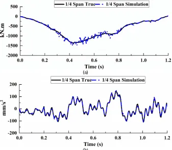
If error level 𝐸𝐸_𝑝𝑝= 0.1, the simulation of the bending moment and acceleration responses at 1/4 span of the simply

supported beam are shown in Fig. 3. The illustration results show that bending moment responses are more likely to

be disturbed by white noise than the acceleration responsesdue to the magnitude of bending moment responses in the

high frequency range is very small compared with the magnitude of acceleration responses (Law et al., 2001). Due to

the larger differences between the simulation responses and the true responses of bending moment responses, it is

more difficult to identify the moving force from the bending moment responses and the identification accuracy should

be relatively poor compared with acceleration responses.

(a)

(b)

Fig. 3. The true responses and simulation responses at 1/4 span for moving force identification with 10% error level: (a) Bending moment responses; (b) Accelerationresponses.

8

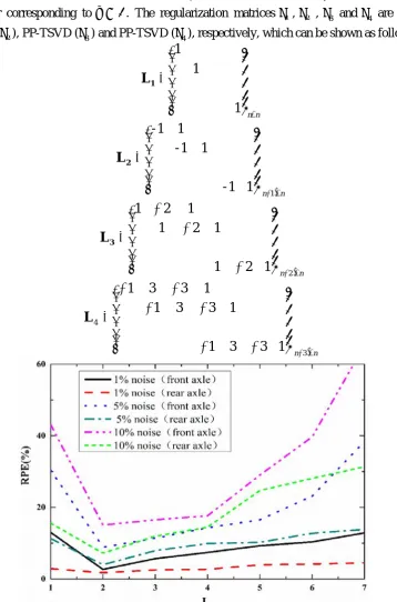
In this section, the regularization matrix 𝐋𝐋 of the PP-TSVD will be chosen in MFI with different cases. As

mentioned above, 𝐋𝐋 is �𝑛𝑛 −(𝑝𝑝 −1)�×𝑛𝑛 and a band matrix, the 𝑝𝑝 is corresponding to (𝑝𝑝 −1)-th derivative operator.

Moreover, if 𝑝𝑝= 1 such that 𝐋𝐋₁ is the unity matrix, then the PP-TSVD is similar to TSVD in this case. If 𝑝𝑝= 2 such that 𝐋𝐋₂approximates the first derivative operator, then the solution of PP-TSVD 𝐀𝐀_{𝐋𝐋,𝑘𝑘}represents a piecewise constant function with at most 𝑘𝑘 discontinuities. If 𝑝𝑝 = 3 such that 𝐋𝐋₃approximates the second derivative operator, then 𝐀𝐀_{𝐋𝐋,𝑘𝑘}

represents a continuous function consisting of at most 𝑘𝑘 −1 straight lines. The 𝐋𝐋₄ is approximations to the third

derivative operator corresponding to 𝑝𝑝= 4. The regularization matrices 𝐋𝐋₁,𝐋𝐋₂ , 𝐋𝐋₃ and𝐋𝐋₄ are corresponding to

TSVD, PP-TSVD (𝐋𝐋₂), PP-TSVD (𝐋𝐋₃) and PP-TSVD (𝐋𝐋₄), respectively, which can be shown as follows

n n×             = 1 1 1  1 L

(n−)×n

            = 1 1 1 -1 1 -1 1 -  2 L

(n− )×n

            − − − = 2 1 2 1 1 2 1 1 2 1    3

L (27)

(n− )×n

            − − − − − − = 3 4 1 3 3 1 1 3 3 1 1 3 3 1     L

Fig. 4. MFI by PP-TSVD with different regularization matrices using responses at 1/4m, 1/4a and 1/2a

The RPE values of biaxial time-varying forces identified from combined responses (1/4m&1/4a&1/2a) by

PP-TSVD with different regularization matrices are shown in Fig. 4. The illustration results show that the RPE values

change little with regularization matrix 𝐋𝐋 from the 𝐋𝐋₁ to 𝐋𝐋₇ when 1% noise level adopted. However, when larger noise

levels such as 5% and 10% are used, the RPE values are increased significantly especially for higher-order derivative

9

immunity than other derivative operators. We have simulated this problem with different moving force identification

examples and found that the regularization matrix L2 of PP-TSVD is always the optimal which can be used in real

applications directly.

Table 1

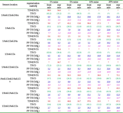
Comparison on RPE(%) values identified by TDM(SVD), TSVD and PP-TSVD with two kinds of regularization matrices

Sensors location regularization

matrix𝐋𝐋

1% noise 5% noise 10% noise 20% noise

front axle rear axle front axle rear axle front axle rear axle front axle rear axle 1/4m&1/2m&3/4m

TDM(SVD) 98.0 56.6 * * * * * *

TSVD (65.2) (35.2) (*) (86.3) (*) (*) (*) (*)

PP-TSVD(𝐋𝐋2) 6.0 5.1 18.8 11.1 19.6 17.0 24.1 21.5

PP-TSVD(𝐋𝐋₃) 9.5 5.5 22.3 11.4 29.4 17.1 40.8 28.0

1/4a&1/2a

TDM(SVD) 9.0 2.7 45.2 13.6 90.4 27.3 * 54.6

TSVD (8.1) (2.5) (28.5) (12.0) (43.3) (13.2) (42.5) (26.7)

PP-TSVD(𝐋𝐋₂) 2.9 1.0 7.9 5.6 14.7 6.3 23.8 11.2

PP-TSVD(𝐋𝐋3) 7.7 1.2 16.8 6.4 23.3 8.7 39.3 9.7

1/4a&1/2a&3/4a

TDM(SVD) 0.6 0.3 2.5 1.4 5.1 2.8 10.2 5.5

TSVD (0.6) (0.3) (2.5) (1.4) (5.1) (2.8) (10.2) (5.5)

PP-TSVD(𝐋𝐋2) 0.6 0.3 2.5 1.4 5.1 2.8 10.2 5.5

PP-TSVD(𝐋𝐋3) 0.6 0.3 2.5 1.4 5.1 2.8 10.2 5.5

1/2m&1/2a

TDM(SVD) * 58.4 * * * * * *

TSVD (83.0) (36.4) (*) (62.9) (*) (63.0) (*) (65.6)

PP-TSVD(𝐋𝐋2) 6.5 4.5 14.1 8.8 19.3 10.9 32.0 11.6

PP-TSVD(𝐋𝐋₃) 8.6 8.9 14.7 14.4 29.2 14.6 49.1 19.5

1/4m&1/2m&1/2a

TDM(SVD) * 30.7 * * * * * *

TSVD (72.3) (25.1) (92.5) (59.8) (92.0) (63.2) (99.9) (69.7)

PP-TSVD(𝐋𝐋2) 5.2 2.1 10.3 8.3 16.9 11.1 32.6 14.2

PP-TSVD(𝐋𝐋3) 5.3 6.8 12.6 10.7 22.9 12.8 43.9 18.5

1/4m&1/2m&1/4a&1/2 a

TDM(SVD) 10.1 3.6 50.3 18.0 * 36.0 * 72.1

TSVD (9.7) (3.0) (26.3) (11.6) (42.3) (18.0) (46.7) (28.3)

PP-TSVD(𝐋𝐋2) 2.4 1.3 8.8 3.3 13.5 6.1 25.8 11.8

PP-TSVD(𝐋𝐋₃) 8.0 1.3 11.5 3.9 19.5 6.8 35.7 13.1

1/4m&1/4a&1/2a

TDM(SVD) 9.7 2.3 40.5 10.9 96.9 21.8 * 43.5

TSVD (9.0) (1.9) (30.4) (10.3) (43.1) (15.6) (41.9) (29.7)

PP-TSVD(𝐋𝐋₂) 2.6 1.7 8.9 4.0 15.1 7.2 25.5 12.3

PP-TSVD(𝐋𝐋3) 7.4 1.8 12.1 4.5 19.4 8.4 32.1 12.7

1/2m&1/4a&1/2a

TDM(SVD) 9.8 3.3 48.8 16.7 97.6 33.5 * 67.2

TSVD (9.6) (2.8) (26.9) (11.1) (45.1) (13.2) (47.3) (26.9)

PP-TSVD(𝐋𝐋2) 2.7 1.3 9.5 2.3 16.3 5.7 25.1 10.8

PP-TSVD(𝐋𝐋3) 5.5 1.5 13.4 2.5 21.5 6.6 33.9 38.3

TDM: time domain method; SVD: singular value decomposition; TSVD: truncated singular value decomposition; PP-TSVD: piecewise polynomial truncated singular value decomposition.

1/4, 1/2, and 3/4 represent the measurement location at a quarter, middle span, and three quarters, respectively. The letters ‘‘m’’ and ‘‘a’’ represent the bending moment and acceleration responses, respectively. Underlined RPE(%) values are for PP-TSVD with double diagonal matrix 𝐋𝐋2, italics RPE(%) values are for PP-TSVD with tri-diagonal matrix 𝐋𝐋3, RPE(%) values in parentheses are for TSVD with unity matrix

𝐋𝐋1, and other values are for conventional counterpart SVD embedded in TDM. The symbol ‘‘*’’ represents that the RPE(%) value is bigger than 100%.

There are 8 cases in Table 1 for evaluating the identification accuracy of TDM(SVD), TSVD and PP-TSVD with

two kinds of regularization matrices. The identification results of rear axle force are better than front axle force in all

cases due to the weight of the front axle is less than half of the rear axle. Due to the bridge weight remains the same,

the heavier the axle is, the greater the mass ratio of axle-bridge will be, and then the greater the dynamic responses

will be. The identification accuracy is improved with the increase of the mass ratio of axle-bridge or the increase of

the dynamic responses.

As shown in Table 1, most of the RPE(%) values of TDM(SVD) are bigger than 90% when white noise level

reaches 10%. The identification accuracy of TSVD has obvious improved compared with TDM(SVD). Moreover, the

10

the PP-TSVD has excellent theoretical completeness and the ability to offset the disadvantage of TSVD perfectly by

extracting the true responses from truncated small singular values and superposes it into the solution of TSVD.

When noise level reaches 20%, the PP-TSVD with regularization matrix 𝐋𝐋₃has quite precise identification results

and the biggest RPE value is less than 50% in all cases, which has higher identification accuracy and stronger

robustness compared with TSVD. Moreover, the PP-TSVD with regularization matrix 𝐋𝐋₂ has very precise

identification results and the biggest RPE value is less than 35% in all cases with 20% noise level, which has much

better identification results compared with PP-TSVD(𝐋𝐋₃). The results show that the regularization matrix is very

important to the PP-TSVD, which affects the identification accuracy and robustness of the PP-TSVD in MFI.

The identified front axle force and rear axle force with different responses and noise levels are shown in Fig. 5 to

Fig. 10. Illustration results show that the identified forces and PSD curves agree well with the true forces in all cases

except for the case of TSVD which has significant deviation when bending moment responses used alone. In this case,

quite a lot of small singular values have been truncated by TSVD method and then the over-fitting problem is revealed.

By choosing the optimal regularization matrix 𝐋𝐋₂, the PP-TSVD has better adaptability with sensors location as shown

in the forces identification results and PSD curves from Fig. 5 to Fig. 10, which also has better noise immunity and

robust with ill-posed problems. Finally, the optimal regularization matrix for the PP-TSVD is 𝐋𝐋₂ and it will be

adopted in the following studies. In this section, the best truncating point 𝑘𝑘 of the PP-TSVD algorithm is default used

in all cases and the selection of the optimal truncating point 𝑘𝑘 of the PP-TSVD will be studied in the next section.

(a)

(b)

11

(a)

(b)

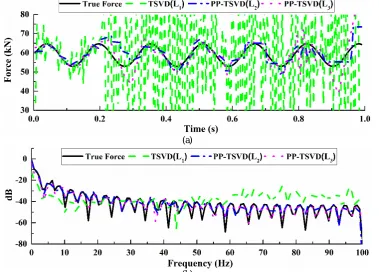
Fig. 6. The identified rear axle force from bending moment responses by TSVD and PP-TSVD with two kinds of regularization matrices (1/4m&1/2m&3/4m 1% Noise): (a) The rear axle force; (b) The PSD of the rear axle.

(a)

(b)

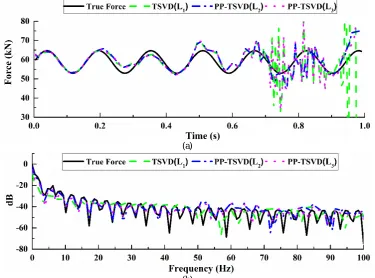
Fig. 7. The identified front axle force from combined responses by TSVD and PP-TSVD with two kinds of regularization matrices (1/4m&1/4a&1/2a 5% Noise): (a) The front axle force; (b) The PSD of the front axle.

(a)

12

Fig. 8. The identified rear axle force from combined responses by TSVD and PP-TSVD with two kinds of regularization matrices (1/4m&1/4a&1/2a 5% Noise): (a) The rear axle force; (b) The PSD of the rear axle.

(a)

(b)

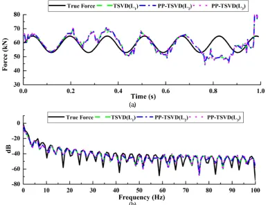
Fig. 9. The identified front axle force from acceleration responses by TSVD and PP-TSVD with two kinds of regularization matrices (1/4a&1/2a&3/4a 20% Noise): (a) The front axle force; (b) The PSD of the front axle.

(a)

(b)

Fig. 10. The identified rear axle force from acceleration responses by TSVD and PP-TSVD with two kinds of regularization matrices (1/4a&1/2a&3/4a 20% Noise): (a) The rear axle force; (b) The PSD of the rear axle.

3.3 Choosing the optimal truncating point k of PP-TSVD

The truncating point 𝑘𝑘 controls the amount of stabilization imposed on 𝐀𝐀_𝑘𝑘 and the calculation accuracy of TSVD.

13

the total number of samples 𝑛𝑛 is 396 and 𝑛𝑛= 396≥ 𝑘𝑘 ≥1. Especially, when 𝑘𝑘=𝑛𝑛 is adopted, no small singular

values are truncated and then the TDM, TSVD, and PP-TSVD show same results. However, when the small singular

values are truncated, there are also some useful responses neglected containing in the small singular values from the

right-hand side 𝐛𝐛. PP-TSVD can overcome this problem of TSVD by extracting the true responses from truncated

small singular values and superposes it into the solution of TSVD.

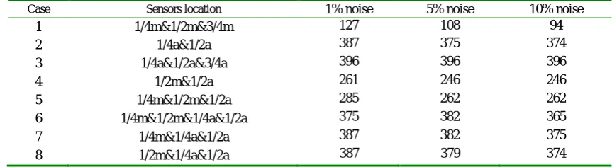
Table 2

The optimal truncating point k of PP-TSVD(𝐋𝐋2) with three kinds of noise level

Case Sensors location 1% noise 5% noise 10% noise

1 1/4m&1/2m&3/4m 127 108 94

2 1/4a&1/2a 387 375 374

3 1/4a&1/2a&3/4a 396 396 396

4 1/2m&1/2a 261 246 246

5 1/4m&1/2m&1/2a 285 262 262

6 1/4m&1/2m&1/4a&1/2a 375 382 365

7 1/4m&1/4a&1/2a 387 382 375

8 1/2m&1/4a&1/2a 387 379 374

Table 2 tabulates the optimal truncating point 𝑘𝑘 of the PP-TSVD with three random noise levels in all 8 cases,

which shows the higher the noise level is, the smaller truncating point should be chosen. That is, the greater the

responses are contaminated by measurement errors, the more small singular values need to be truncated.

In addition, the higher the acceleration responses ratio is in the combined responses, the bigger truncating point

should be chosen, which indicates that the noise has less impact on acceleration responses due to their high frequency

characteristic, and then there will be less small singular values contained in matrix 𝐀𝐀. Especially, when MFI from

acceleration responses alone as case 3, the truncating point 𝑘𝑘= 396 is the total number of samples 𝑛𝑛 as shown in Fig.

11, which indicates that the matrix 𝐀𝐀equals to the matrix 𝐀𝐀_𝐤𝐤. That is, no small singular values are truncated and no additional responses are extracted from truncated small singular values. In this case, the identification results and the

PSD curves by TSVD and PP-TSVD are the same, as shown in Table 1 and Fig. 9 to Fig. 10.

In contrast, the higher the bending moment responses ratio is in the combined responses, the smaller truncating point

should be chosen, which indicates that the noise has more impact on bending moment responses due to their low

frequency characteristic, and then more small singular values need to be truncated. In this case, it is obviously

necessary to extract the true responses from truncated small singular values by the PP-TSVD, and then the

identification results and the RPE values are much improved compared with the TSVD as modification value −𝐕𝐕_𝑘𝑘𝐰𝐰_𝑘𝑘. As shown in Fig. 12, when acceleration responses used alone in MFI, most of measured responses are useful and the

number of the small values is very small. However, if the truncating point 𝑘𝑘 is taken at 396 the RPE values will be

increased sharply due to very ill-posed matrix of 𝐀𝐀 which is caused by small singular values. Therefore, it is obviously

important to truncate very small singular values of matrix 𝐀𝐀, even if the number is very small.

As shown in Fig. 13, when bending moment and acceleration responses are both used in the combined responses, RPE values are increased dramatically when the truncating point 𝑘𝑘 is greater than 250. Moreover, there is a typical

crest when the truncating point near 100, which also should be avoided to maintain reasonable RPE values of MFI.

As shown in Fig. 14, when bending moment responses used alone in MFI, RPE values are increased dramatically

when the truncating point 𝑘𝑘 is bigger than 100. In this case, the optimal truncating point 𝑘𝑘 is very small and then there

are many small singular values that need to be truncated. Therefore, the identification results of PP-TSVD are much

improved than TSVD by extracting the true responses and superposing it into the solution of TSVD as in Table 1 and

Fig. 5 to Fig. 6.

In summary, the type of sensors has great influence on the selection of the optimal truncation parameter 𝑘𝑘.

14

if the truncating point 𝑘𝑘 is small, there are many useful responses that can be extracted from truncated small singular

values and then the identification accuracy of PP-TSVD is superior than that of TSVD. On the contrary, if the

truncating point 𝑘𝑘 is large and close to the total number of samples 𝑛𝑛, there would be only few useful responses to be

extracted and the improvement made by PP-TSVD becomes modest compared with TSVD.

Fig. 11. Influence of truncating point k of PP-TSVD on MFI from acceleration responses (1/4a&1/2a&3/4a)

Fig. 12. Influence of truncating point k of PP-TSVD on MFI from acceleration responses (1/4a&1/2a)

15

Fig. 14. Influence of truncating point k of PP-TSVD on MFI from bending moment responses (1/4m&1/2m&3/4m)

4 Conclusions

In this work, a novel algorithm called PP-TSVD was introduced in MFI and a comparative study was made to

evaluate this technique against TSVD and the SVD embedded in the TDM. By means of numerical simulations, a

comprehensive parametric study has been done and the following conclusions can be drawn:

By truncating small singular values to improve the condition of matrix 𝐀𝐀, the TSVD can partially solve the

ill-posed problem occurred with the SVD-based methods such as TDM due to the impact of small singular values. Even

though TSVD can cope reasonably well with the ill-posed problem in MFI process, its accuracy is still not very good

as this technique ignores all the 𝑛𝑛 − 𝑘𝑘 small singular values which contain some useful responses. The PP-TSVD can

not only solve ill-posed problem as TSVD, but also extracts the true responses and superposes it into the solution of

TSVD as a modification value, which has excellent theoretical completeness and offset the disadvantage of TSVD

perfectly.

By choosing the optimal regularization matrix, the PP-TSVD has better adaptability with different type of

responses (acceleration, bending moment or their combination) and number of sensors. This technique also has better

noise immunity and robust with ill-posed problems. Thefirst derivative operator 𝐋𝐋₂ has much better noise immunity

than other derivative operators, which will serve as the optimal regularization matrix for the PP-TSVD.

Finally, it is found that the identification accuracy and ill-posed immunity of the PP-TSVD is also influenced by the

truncating point 𝑘𝑘, which shows that for the higher of the noise level, the smaller truncating point should be chosen to

enhance the accuracy of the technique. When the optimal truncating point k is 396 which equals to the total number of

samples 𝑛𝑛 in this special case 3, no small singular values are truncated and then the ill-posed immunity of PP-TSVD

can not be reflected. In this case, all methods showed same results regardless of the type of methods such as TDM,

TSVD, and PP-TSVD. In practical implementation of MFI, there must be some small singular values that need to be

truncated because the total number of samples will be a much larger number compared with the simple numerical

simulation. In this circumstance, PP-TSVD will be superior to other methods. Acceleration responses or combination

responses were shown to facilitate more accurate MFI by PP-TSVD hence they are highly recommended as the main

response data for use with the PP-TSVD based MFI procedure. Due to their low frequency characteristic and possible

16 Acknowledgments

This work is supported by the Key Science and Technology Program of Henan Province, China (192102310011),

the Science and Technology Innovation Team of Eco-building Material and Structural Engineering in the University

of Henan Province, China (13IRTSTHN002), and the University-industry Collaboration Project of Henan Province,

China (142107000088).

References:

Bouhamidi A, Jbilou K, Reichel L, et al. (2011) An extrapolated TSVD method for linear discrete ill-posed problems with Kronecker structure.

Linear Algebra and Its Applications 434(7): 1677-1688.

Busby HR and Trujillo DM (1997) Optimal regularization of an inverse dynamics problem. Computers & structures 63(2): 243-248.

Chan THT and Ashebo DB (2006) Theoretical study of moving force identification on continuous bridges. Journal of sound and Vibration

295(3-5): 870-883.

Chan THT, Law SS, Yung TH, et al. (1999) An interpretive method for moving force identification. Journal of sound and vibration 219(3): 503-524.

Chan THT, Yu L, Law SS, et al. (2001) Moving force identification studies, I: theory. Journal of Sound and Vibration 247(1): 59-76.

Chen Z and Chan THT (2017) A truncated generalized singular value decomposition algorithm for moving force identification with ill-posed problems. Journal of Sound and Vibration 401: 297-310.

Chen Z, Chan THT and Nguyen A (2018) Moving force identification based on modified preconditioned conjugate gradient method. Journal of Sound and Vibration 423: 100-117.

Choi HG, Thite AN and Thompson DJ (2007) Comparison of methods for parameter selection in Tikhonov regularization with application to inverse force determination. Journal of Sound and Vibration 304(3-5): 894-917.

Ding Y, Zhao BY, Wu B, et al. (2015) Simultaneous identification of structural parameter and external excitation with an improved unscented Kalman filter. Advances in Structural Engineering 18(11): 1981-1998.

Dowling J, OBrien EJ and González A (2012) Adaptation of Cross Entropy optimisation to a dynamic Bridge WIM calibration problem.

Engineering Structures 44: 13-22.

Feng DM, Sun H and Feng MQ (2015) Simultaneous identification of bridge structural parameters and vehicle loads. Computers & Structures

157: 76-88.

Giustolisi O (2004) Sparse solution in training artificial neural networks. Neurocomputing 56: 285-304.

Hansen PC and Mosegaard K (1996) Piecewise polynomial solutions without a priori break points. Numerical linear algebra with applications

3(6): 513-524.

Law SS, Chan THT and Zeng QH (1999) Moving force identification-a frequency and time domains analysis. Journal of dynamic systems, measurement and control 121(3): 394-401.

Law SS, Chan THT and Zeng QH (1997) Moving force identification: a time domain method. Journal of Sound and vibration 201(1): 1-22. Law SS, Chan THT, Zhu QX, et al. (2001) Regularization in moving force identification. Journal of Engineering Mechanics 127(2): 136-148. Li J, Law SS and Hao H (2013) Improved damage identification in bridge structures subject to moving loads: numerical and experimental

studies. International Journal of Mechanical Sciences 74: 99-111.

Liu J, Meng XH, Zhang DQ, Jiang C, et al. (2017) An efficient method to reduce ill-posedness for structural dynamic load identification.

Mechanical Systems and Signal Processing 95: 273-285.

Liu J, Sun XS, Han X, et al. (2015) Dynamic load identification for stochastic structures based on Gegenbauer polynomial approximation and regularization method. Mechanical Systems and Signal Processing 56: 35-54.

Lu ZR and Liu JK (2011) Identification of both structural damages in bridge deck and vehicular parameters using measured dynamic responses.

Computers & Structures 89(13-14): 1397-1405.

O'Connor C and Chan THT (1988) Dynamic wheel loads from bridge strains. Journal of Structural Engineering 114(8): 1703-1723.

Pan CD, Yu L, Liu HL, et al. (2018) Moving force identification based on redundant concatenated dictionary and weighted l1-norm

regularization. Mechanical Systems and Signal Processing 98: 32-49.

Pinkaew T (2006) Identification of vehicle axle loads from bridge responses using updated static component technique. Engineering Structures

28(11): 1599-1608.

Ronasi H, Johansson H and Larsson F (2011) A numerical framework for load identification and regularization with application to rolling disc problem. Computers & structures 89(1-2): 38-47.

Sanchez J and Benaroya H (2014) Review of force reconstruction techniques. Journal of Sound and Vibration 333(14): 2999-3018.

Sobouti A, Motagh M and Sharifi MA (2016) Inversion of surface gravity data for 3-D density modeling of geologic structures using total variation regularization. Studia Geophysica et Geodaetica 60(1): 69-90.

Winkler JR (1997a) Polynomial basis conversion made stable by truncated singular value decomposition. Applied Mathematical Modelling 21(9): 557-568.

Winkler JR (1997b) Tikhonov regularisation in standard form for polynomial basis conversion. Applied Mathematical Modelling 21(10): 651-662.

Xu PL (1998) Truncated SVD methods for discrete linear ill-posed problems. Geophysical Journal International 135(2): 505-514. Yu L and Chan THT (2007) Recent research on identification of moving loads on bridges. Journal of Sound and Vibration 305(1-2): 3-21. Yu L, Chan THT and Zhu JH (2008) A MOM-based algorithm for moving force identification: Part II-Experiment and comparative studies.

Structural Engineering and Mechanics 29(2): 155-169.

Yu Y, Cai CS and Deng L (2016) State-of-the-art review on bridge weigh-in-motion technology. Advances in Structural Engineering 19(9): 1514-1530.

Zhu XQ and Law SS (2006) Moving load identification on multi-span continuous bridges with elastic bearings. Mechanical Systems and Signal Processing 20(7): 1759-1782.