ANALYSIS OF FAULTS IN THREE PHASE VOLTAGE SOURCE INVERTER
NURUL ASSHIKIN BINTI KASIM
A report submitted in partial fulfillment of the requirement for the degree of Electrical
Engineering in Power Electronic and Drive
Faculty of Electrical Engineering
UNIVERSITI TEKNIKAL MALAYSIA MELAKA
i
ABSTRACT
ii
ABSTRAK
Projek ini menganalisis tentang kerosakan yang berlaku dalam penyongsang sumber voltan
tiga fasa. Penyongsang sumber voltan digunakan secara meluas dalam aplikasi pemacu motor
dan kualiti kuasa. Majoriti kerosakan berkaitan dengan suis kuasa, seperti kerosakan litar
terbuka dan litar pintas. Pernyataan masalah projek ini adalah kos penyelenggaraan yang
tinggi, kerosakan kuasa elektronik dan mengganggu proses pembuatan. Kemudian objektif
projek ini adalah mengenal pasti dan menganalisis kerosakan yang dijana menggunakan
teknik ‘fast Fourier transform’ (FFT) dan ‘short-time Fourier transform’ (STFT). Teknik FFT sangat berguna dalam menganalisis harmonik dan ia adalah alat penting bagi reka bentuk
penapis. Ia mempunyai beberapa kelemahan seperti kehilangan maklumat yang berkenaan
dengan masa, jadi ia hanya boleh digunakan dalam keadaan tetap dan tidak boleh
menunjukkan keadaan ini dihasilkan. Manakala STFT berkebolehan dalam isyarat bukan
pegun dan ia telah digunakan dalam analisis kualiti kuasa. Kelebihan teknik ini adalah
keupayaannya untuk memberikan kandungan isyarat harmonik pada setiap tempoh masa.
Tetapi, teknik ini juga mempunyai had lebar window tetap yang keutamaannya dipilih dan ini
menyebabkan had untuk frekuensi rendah dan pada masa yang sama analisis isyarat tidak
bergerak frekuensi yang tinggi. Dalam analisis ini, parameter seperti arus rms (Irms), arus
purata (Iave) dan jumlah herotan harmonik (THD) digunakan untuk mengenal pasti ciri-ciri
iii
ACKNOWLEDGEMENT
ALHAMDULILLAH, I am grateful to God for His blessing and mercy to make this project successful and complete in this semester. First of all, I would like to express to Universiti Teknikal Malaysia Melaka. The special thanks to my helpful supervisor Pn.Norhazilina Binti Bahari for giving invaluable guidance supervision, committed and sustained with patience during this project.
iv
TABLE OF CONTENTS
PAGE
DECLARATION DEDICATION
ABSTRACT i
ABSTRAK ii
ACKNOWLEDGEMENTS iii
TABLE OF CONTENTS iv-vi
LIST OF TABLES vii
LIST OF FIGURES viii-x
LIST OF APPENDICES xi
CHAPTER
1.0 INTRODUCTION 1
1.1 Overview 1
1.2 Project Motivation 2
1.3 Objective 2
1.4 Scope 3
1.5 Report Outline 3
2.0 LITERATURE REVIEW 4
2.1 Theory
2.1.1 Inverter 4
v
2.1.3 Pulse Width Modulation (PWM) 6-7
2.1.4 Short Time Fourier Transform 8-10
2.1.5 Fast Fourier Transform 10-11
2.1.6 Stationary signal and Non-stationary signal 11-12 2.1.7 Detection of fault for voltage source inverter
(VSI)
12-16
2.1.8 Type of fault 16-19
2.2 Related previous work 19-20
2.3 Summary of review 20-21
3.0 DESIGN METHODOLOGY 22
3.0Introduction 22
3.1 Project Methodology
3.1.1 Overall Project Flow Chart 23
3.1.2 Flow Chart of Simulation 24
3.2 Simulation Circuit
3.2.1 Open-circuit Fault 25-26
3.2.2 Short-circuit Fault 27-28 3.3 Analytical Approach
3.3.1 Switching sequence for three-phase inverter output 29-31
3.2.2 Open-circuit fault 31-33
3.2.3 Short circuit fault 33-34
4.0 RESULT AND ANALYSIS
4.1 Short-Time Fourier Transform 35
4.1.1 Time Frequency Representation (TFR) 35-36
4.1.2 Open circuit fault 36-39
4.1.3 Short-circuit fault 39-41
vi
4.2.1 Frequency Spectrum 42
4.2.2 Open-circuit fault 42-48
4.2.3 Short-circuit fault 49-54
5.0 CONCLUSIO N AND RECOMMENDATION 55-56
REFERENCES 57-58
vii
LIST OF TABLE
TABLE PAGE
Table 2.1.: Valid switch states for three-phase VSI 13 Table 4.1: The value of RMS current, average current and THD for open-circuit
fault of the upper switches
42-43
Table 4.2: The value of RMS current, average current and THD for open-circuit fault of the lower switches
46
Table 4.3: The value of RMS current, average current and THD for short-circuit fault of the upper switches
49
Table 4.4: The value of RMS current, average current and THD for short-circuit fault of the lower switches
viii
LIST OF FIGURES
FIGURE PAGE
Figure 2.1: Inverter 5
Figure 2.2 : Three-Phase Half Bridge Inverter 6
Figure 2.3 : Three-Phase Full Bridge Inverter 6
Figure 2.4 : Pulse Width Modulation signal 7
Figure 2.5 : Stationary signal 11
Figure 2.6 : Non-stationary signal 12
Figure 2.7 : Gating signals of inverter 13
Figure 2.8: Switching sequence at state 1 14
Figure 2.9: Switching sequence at state 2 15
Figure 2.10: Gating signals of the inverter in an ideal case 16 Figure 2.11: Gating signals of the inverter in an open-circuit fault (lower) 17 Figure 2.12: Gating signals of the inverter in an open-circuit fault (upper) 18 Figure 2.13: Switching signals of the inverter in short-circuit fault (lower) 18 Figure 2.14: Switching signals of the inverter in short-circuit fault (upper) 19
Figure 3.1: Overall Project Flow Chart 23
Figure 3.2: Flow Chart of Simulation 24
Figure 3.3: Simulation circuit of open-circuit fault (upper) 25 Figure 3.4: Simulation circuit of open-circuit fault (lower) 26 Figure 3.5: Simulation circuit of short-circuit fault (upper) 27 Figure 3.6: Simulation circuit of short-circuit fault (lower) 28
Figure 3.7: Waveforms of comparator voltage 29
ix Figure 3.9: Signal of Open-circuit fault of upper switches 31-32 Figure 3.10: Open-circuit fault of the lower switches 32-33 Figure 3.11: Short-circuit fault of the upper switches 33 Figure 3.12: Short-circuit fault of the lower switches 34 Figure 4.1: Time Frequency Representation of the fault signal for phase A 36 Figure 4.2: Average current of open-circuit fault (upper) 37 Figure 4.3: RMS current of open-circuit fault (upper) 37
Figure 4.4: THD for open-circuit fault (upper) 37
Figure 4.5: Average current of open-circuit fault (lower) 38 Figure 4.6: RMS current of open-circuit fault (lower) 38
Figure 4.7: THD of open-circuit fault (lower) 39
Figure 4.8: Average current of short-circuit fault (upper) 39 Figure 4.9: RMS current of short-circuit fault (upper) 40
Figure 4.10: THD of short-circuit fault (upper) 40
Figure 4.11: Average current of short-circuit fault (lower) 41 Figure 4.12: RMS current of short-circuit fault (lower) 41
Figure 4.13: THD of short-circuit fault (lower) 41
Figure 4.14: Frequency spectrum for phase A 42
xi
LIST OF APPENDICES
APPENDIX TITLE PAGE
A Coding Of Short Time Fourier Transform 59-63
B Coding Of Fast Fourier Transform 64
1
CHAPTER 1
INTRODUCTION
1.1 Overview
Inverter is circuits that convert DC input voltage to symmetric AC output voltage which both magnitude and frequency can be controlled. Voltage source inverters can be classified as an inverter. When input DC voltage remains constant, then it is called voltage source inverter (VSI). In industry, voltage source inverter (VSI) plays role in power supplies, motor drives, power quality application, etc. The percentage of failures in the power converter is estimated about 38% and mostly occur in power switches [1]. To overcome this situation, fast Fourier transform (FFT) and short-time Fourier transform (STFT) technique is used to analyze the signal.
2 1.2 Project Motivation
High cost of maintenance is required when the drive system shuts down due to the fault occurrences. The presence of fault causes damage to the power electronics such as inverter. Furthermore, it also interrupts manufacturing process when the drive system has to be stopped. Fast Fourier Transform (FFT) and Short-Time Fourier Transform (STFT) techniques is used to solve this problem. FFT is an essential tool for filter design and very useful in the analysis of harmonic. It has some drawbacks such as losses of temporal information, so that it can only be used in the steady state and cannot show the moment when the event is produced [4]. STFT is applicable to non-stationary signals and it has been used in power quality analysis. The advantage of this technique is its ability to give the harmonic content of the signal at every time-period specified by a define window. But, this technique also has the limitation of fixed window width chosen a priority and this causes limitation for low-frequency and high-frequency non-stationary signal analysis at the same time [5].
1.3 Objectives
The objective of this project is:
i. To study fault in three-phase voltage source inverter (VSI).
ii. To identify and analyze generated fault using fast Fourier transform (FFT) and short-time Fourier transform (STFT) technique.
3 1.4 Scope
In order to achieve this objective, several scopes have been outlined. In this analysis, Matlab software is used as simulation purpose and RMS current (Irms), average current (Iave) and total harmonic distortion (THD) are used to identify the characteristic of the signals. The technique used in this analysis is fast Fourier transform (FFT) and short-time Fourier transform (STFT). FFT is suitable for stationary signal [6] while STFT is non-stationary signal [7]. The limitation of three-phase inverter is the frequency of the output voltage waveform depends on the switching rate of the semiconductor devices and the upper limit of the frequencies is fixed by the device capability [8].
1.5 Report outlines
After doing some research for this project, this report is written and discuss about the analysis of fault in three phase VSI.
In chapter 1, there will be an introduction about this project, project background, problem statement, the objective, scope and report outlines.
In chapter 2, the literature review will review on the theory, basic principles of the fault and overview of related published results of a fault in voltage source inverter. This chapter also includes the summary of the review.
In chapter 3, the methodology will show the process and simulation approach of fault detection. In chapter 4, the result and discussion will discuss about the whole project.
4
CHAPTER 2
LITERATURE REVIEW
2.1 Theory
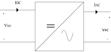
2.1.1 Inverter
The inverters are DC to AC converters. The application of inverter such as standby power supply, induction heating and variable speed AC motor drives [9].
The output voltage of the inverter can be controlled with the help of the drives of the switches. To control the output voltages of the inverter, the pulse width modulation (PWM) technique is used. Some inverters are called as PWM inverters. It contains harmonic whenever it is non-sinusoidal. These harmonics can be reduced by using proper control schemes.
5
=
IDC
+
-VDC
+
-VAC
[image:17.612.217.410.74.164.2]IAC
Figure 2.1: Inverter
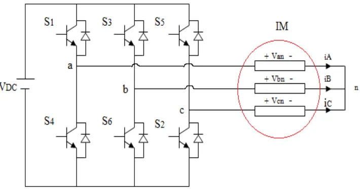
2.1.2 Three-phase Inverter
6
Figure 2.2: Three-Phase Half Bridge Inverter
Figure 2.3: Three-Phase Full Bridge Inverter
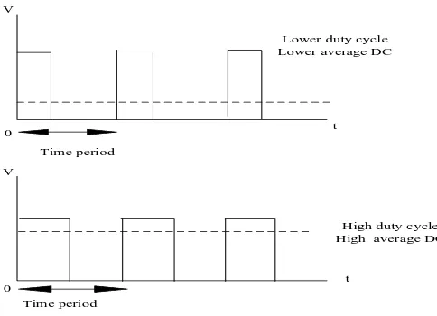
2.1.3 Pulse Width Modulation
[image:18.612.133.488.326.513.2]7 inverter while controlled AC output voltage is obtained by adjusting the on and off periods of the inverter components [11]. The PWM provides a way to decrease the total harmonic distortion (THD) of load current. A PWM inverter output with some filtering can generally meet THD requirements easier than the square wave switching scheme. The unfiltered PWM output will have a relatively high THD, but the harmonics will be at higher frequency than for a square wave, result to ease to be filtered.
Besides, the advantage of PWM for three phase inverter is reduced filter requirements for harmonic reduction and controllability of the amplitude of the fundamental frequency. Then, the other advantages of PWM techniques are the output voltage control with this method can be obtained without any additional components. The lower order harmonics can be eliminated or minimized along with its output voltage control. In most AC motor loads, higher order harmonic voltage distortion can be filtered by the inductive nature of the load itself.
PWM inverter is most popular in industrial application. PWM technique is characterized by constant amplitude pulses. The width of these pulses is however modulated to obtain inverter output voltage control and reduce. The figure below shows the pulse width modulated signal.
V
t
t V
Time period
Time period
Lower duty cycle Lower average DC
High duty cycle High average DC
[image:19.612.191.433.473.648.2]0 0
8 2.1.4 Short-Time Fourier Transform
The short-time Fourier transform (STFT) is a transform. It involves both time and frequency and allows a time-frequency analysis [12]. The time-frequency analysis is motivated by the analysis of non-stationary signal that is characteristic of the spectrum is changing in time [13]. The objective of STFT is to capture the time variation in the frequency content of the signal. It represents a compromise between time and frequency based on signal perspectives and it also provides some information about when and what events occur. The basic principle of STFT is to slice up the signal into suitable overlapping time segments and then to perform a Fourier analysis on each slice to ascertain the frequencies contained in it [7]. It is defined as in Equation 2.1.
S
t, f x
w
t
e
j2ftd
(2.1)
x is the input signal and w
t is the window function. Some limitation of STFT is window length. In STFT, narrow window gives good resolution in time but poor resolution in frequency. Wide window gives good resolution in frequency but poor resolution in time [14].2.1.4.1 Performance Parameter
i. Instantaneous Average Current
Instantaneous Average Current is the mean value of a signal that corresponds to a specific time, t and it can calculate as:
x
w
t
d
T t
T
ave
I
0
1
.(2.2)
9 ii. Instantaneous RMS Current
df ff t S t
I
rms
max0
, (2.3)
t fS , is the time-frequency representation (TFR) of the signal and
f
maxis the maximum
frequency
iii. Instantaneous RMS Fundamental Current
dff f f t S t h i lo
I
1rms 2
, (2.4)
2
1
f
f
f
hi (2.5)
2 1
f
f
f
lo (2.6)Where
f
1is the fundamental frequency that corresponds to the power system frequency and
f
is the bandwidth.
iv. Instantaneous Total Harmonic Distortion
t tI
t
I
I
rms Hh hrms THD 1 2 2 ,
10
tI
h,rms is the RMS harmonic current and H is the highest measured harmonic component.2.1.5 Fast Fourier Transform
Fourier transform is mathematical technique which convert the signal from time to frequency domain. It is very useful for many applications where the signals are stationary, as in diagnostic faults of electrical machines [6]. The stationary signal is frequency or spectral contents are not changing with respect to time. Function of fast Fourier transform (FFT) is localized in the frequency domain; providing the user useful information on the operating conditions of the power distribution network. Not advisable to apply a methodology associated with FFT as the analysis tool if the signal is a stationary signal associated with a wide range of frequencies superimposed to the power frequency component. FFT has various obstacles and limitations associated with time-frequency resolution where it is not possible to identify at what times these high frequency components occurred [15]. It can be defined as:
X
f
x
t
e
j2fttdt
(2.8)) (t
x is the signal of interest, t is the time and f is the signal frequency.
2.1.5.1Performance Parameter
i. Current Measurement
1 0 1 N nrms
i
n
11 ii. Instantaneous Total Harmonic Distortion
t t
I
t
I
I
rms H
h hrms THD
1 2
2 ,
(2.10)
tI
h,rms is the RMS harmonic current and H is the highest measured harmonic component.2.1.6 Stationary Signal and Non-stationary Signal
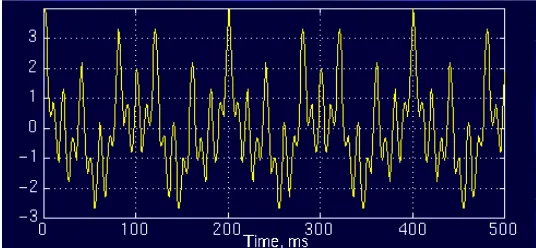
Stationary signal is a signal whose frequency content does not change in time. In this signal all frequency components exist at all time [16]. There is 10 Hz , 50 Hz and 100 Hz at all time.
Example for stationary signal. It has frequencies of 10, 25, 50 and 100 Hz at a given time instant. The signal is plotted in Figure 2.5.
[image:23.612.178.446.486.610.2]x(t) = cos (2*pi*10*t) + cos (2*pi*25*t) + cos (2*pi*50*t) + cos (2*pi*100*t)
Figure 2.5: Example of stationary signal
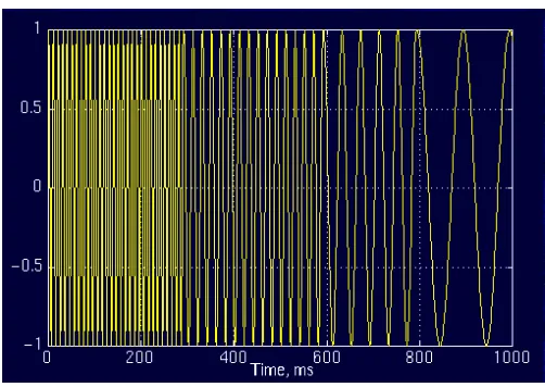
12 different time intervals. The interval 0 to 300 ms has a 100 Hz sinusoid, the interval 300 to 600 ms has a 50 Hz sinusoid, the interval 600 to 800 ms has a 26 Hz sinusoid and lastly the interval 800 to 1000 ms has a 10 Hz sinusoid. In this signals the frequency components do not appear at all time.
Figure 2.6: Example of non-stationary signal
2.1.7 Detection of Fault for Voltage Source Inverter (VSI)
2.1.7.1 Switching Function Model for VSI