A symmetric integrated radial basis function method for
solving differential equations
N. Mai-Duy
∗, D. Dalal, T.T.V. Le, D. Ngo-Cong and T. Tran-Cong
Computational Engineering and Science Research Centre,
School of Mechanical and Electrical Engineering,
University of Southern Queensland, Toowoomba, QLD 4350, Australia
Submitted to
Numerical Methods for Partial Differential Equations,
March/2017; revised, November/2017
AbstractIn this paper, integrated radial basis functions (IRBFs) are employed for Hermite
interpolation in the solution of differential equations, resulting in a new meshless symmetric
RBF method. Both global and local approximation-based schemes are derived. For the
latter, the focus is on the construction of compact approximation stencils, where a sparse
system matrix and a high-order accuracy can be achieved together. Cartesian-grid-based
stencils are possible for problems defined on non-rectangular domains. Furthermore, the
effects of the RBF width on the solution accuracy for a given grid size are fully explored
with a reasonable computational cost. The proposed schemes are numerically verified in some
elliptic boundary-value problems governed by the Poisson and convection-diffusion equations.
High levels of the solution accuracy are obtained using relatively coarse discretisations.
Keywords: Hermite interpolation, global approximation, compact local approximation,
in-tegrated radial basis function, flat radial basis function, extended precision
∗Corresponding author E-mail: [email protected], Telephone 46312748, Fax
1
Introduction
Radial basis function (RBF) methods have become a powerful means of representing
func-tions and solving ordinary/partial differential equafunc-tions (ODEs/PDEs). For strict
interpola-tion (noiseless data), a target funcinterpola-tion can be represented by a linear combinainterpola-tion of RBFs.
According to Micchelli’s theorem [1], for a large class of RBFs, their interpolation
matri-ces constructed from the distinct data points are guaranteed to be invertible. Examples of
RBFs that are covered by Micchelli’s theorem and of particular interest in practice are the
multiquadric, inverse multiquadric and Gaussian functions. Unlike conventional
interpola-tion schemes, the quality of approximainterpola-tions based on these infinitely smooth RBFs can be
controlled not only by the number of data points (i.e. the number of RBFs) but also by the
RBF widths (also called the free/shape parameters). Furthermore, RBF methods are
capa-ble of yielding spectral accuracy with respect to the number of RBFs and/or their widths [2].
Application of RBFs to the numerical solution of PDEs was proposed by Kansa in 1990 [3].
In Kansa’s method, the PDE is discretised by means of point collocation and a field variable
is approximated by a set of multiquadric functions with a differentiation process being
em-ployed to obtain basis functions for derivative terms in the PDE (DRBFs). Since then, the
RBF solution to differential problems has received a great deal of attention (see, e.g., [4-14]).
For a given node distribution, the solution accuracy can still be improved by changing the
value of the RBF width. Finding the optimal RBF width for a general case still presents a
great challenge. In practice, one may rely on numerical algorithms such as those based on
statistics (cross validation and maximum likelihood estimation) for determining this value.
For a smooth function, the best accuracy can often be achieved at a large RBF width (i.e.
near-flat RBF). As the RBF width increases, its matrix condition number grows rapidly
and one needs stable-calculation algorithms for obtaining a reliable numerical solution (see,
e.g., [15-20]). The issue of stagnation errors (i.e. failure of convergence under continuing
node refinement) was recently discussed in [21] along with several treatments proposed to
overcome it. It should be noted that the system matrix resulting from Kansa’s method may
not be invertible for certain configurations of RBF centres and certain kinds of differential
For data containing both function and derivative values, one can employ the RBF Hermite
interpolation approach [23-25]. Its applications in the solution of ODEs/PDEs were reported
in, e.g., [26-28]. The main advantage of this approach is that it can yield an interpolation
matrix that is symmetric and invertible for both function representation and solution of
ODEs/PDEs. The symmetric property also allows for the saving of computer storage space
and the use of a more efficient algebraic solver. In addition, the RBF Hermite interpolation
approach was also utilised to construct compact local approximations (see, e.g., [29,16,30]).
This kind of application has attracted more attention in recent years as both a sparse system
matrix and a fast convergence rate of the solution can be achieved together.
Integrated RBFs (IRBFs) have been proposed for solving ODEs/PDEs (see, e.g., [31-35,4]).
In IRBF methods, basis functions used for the approximation of a field variable are obtained
by integrating RBFs. Numerical experiments showed that IRBF methods can yield an
im-proved rate of convergence. In previous reports [30,36,37], we integrated RBFs with respect
to the Cartesian coordinates (i.e. x, y and z). Through integration constants, nodal
deriva-tive values can be incorporated into the IRBF expressions. Their associated basis functions
are generally not radial and the resultant IRBF matrices are nonsymmetric. In this work,
RBFs are integrated with respect to the radius without the addition of integration constants.
All derived basis functions are radial and they are employed for Hermite interpolation. Both
global and local approximations are considered, producing new strong forms of the IRBF
approach. For the former, the interpolation at a point involves function values at all nodes
and therefore its system matrix is fully populated. For the latter, compact IRBF
approx-imations are constructed on small stencils, resulting in a sparse system matrix. For both
versions, the interpolation matrix is symmetric. The obtained IRBF results are compared
with those by the classical finite-difference methods (FDMs), compact FDMs, and Hermite
methods based on differentiated RBFs. The rest of the paper is organised as follows. In
Section 2, relevant basis functions for DRBFs and IRBFs are provided. Global and local
schemes of the proposed IRBF Hermite-based method are presented and verified in Sections
3 and 4, respectively. Section 5 gives some concluding remarks. In Appendix, the process
of acquiring the limit of the fourth-order cross derivative as the radius approaches zero is
2
Basis functions for DRBFs and IRBFs
For DRBFs, a function can be represented by a linear combination of RBFs
f(x) = N
X
j=1
wjϕ(kx−xjk), (1)
where N is the number of given data points, {ϕ(r =kx−xjk)}Nj=1 a set of RBFs, {xj}Nj=1 a
set of centres which is normally chosen to be the same as a set of data points, and {wj}Nj=1
a set of weights to be found. It has been theoretically shown that the interpolation matrix
derived from (1) on a set of distinct points is nonsingular if ϕ is a positive definite function
such as the inverse multiquadric and Gaussian functions, or a conditionally positive definite
function of order 1 such as the multiquadric function [1]. In this work, RBF is taken as the
multiquadric (MQ) function
ϕ(r) =√r2+a2, (2)
where a is the MQ width.
Derivatives of function f can then be determined as, e.g., in two dimensions
∂kf(x)
∂xk = N
X
j=1
wj
∂kϕ(kx−x jk)
∂xk , k = 1,2,3,· · ·, (3)
∂kf(x)
∂yk = N
X
j=1
wj
∂kϕ(kx−x jk)
∂yk , k = 1,2,3,· · ·, (4)
∂kf(x)
∂xm∂yn = N
X
j=1
wj
∂kϕ(kx−x jk)
∂xm∂yn , m = 1,2,· · ·, n = 1,2,· · · , k=m+n. (5)
Expressions for computing derivatives of (2) with respect to r up to the fourth order are
dϕ dr =
r
√
r2+a2, (6)
d2ϕ
dr2 =
a2
(r2+a2)3/2, (7)
d3ϕ
dr3 = −
3a2r
(r2+a2)5/2, (8)
d4ϕ
dr4 = −
3a2(a2−4r2)
For IRBFs, a function is decomposed into a set of basis functions that are obtained from
integrating (2) with respect to r. Below is the case, where the MQ is integrated 4 times
¯
ϕ(r) =
a4 45 −
83a2r2
720 +
r4 120
√
r2+a2+
−a
4r 16 +
a2r3 12
ln r+
√
r2+a2
a
!
, (10)
dϕ¯
dr =
−13a
2r
48 +
r3 24
√
r2+a2 +
−a
4
16 +
a2r2 4
ln r+
√
r2+a2
a
!
, (11)
d2ϕ¯
dr2 =
−a 2 3 + r2 6 √
r2+a2 +a 2r 2 ln
r+√r2+a2
a
!
, (12)
d3ϕ¯
dr3 =
r
2
√
r2+a2+a 2
2 ln
r+√r2+a2
a
!
, (13)
d4ϕ¯
dr4 =
√
[image:5.612.100.551.87.320.2]r2+a2. (14)
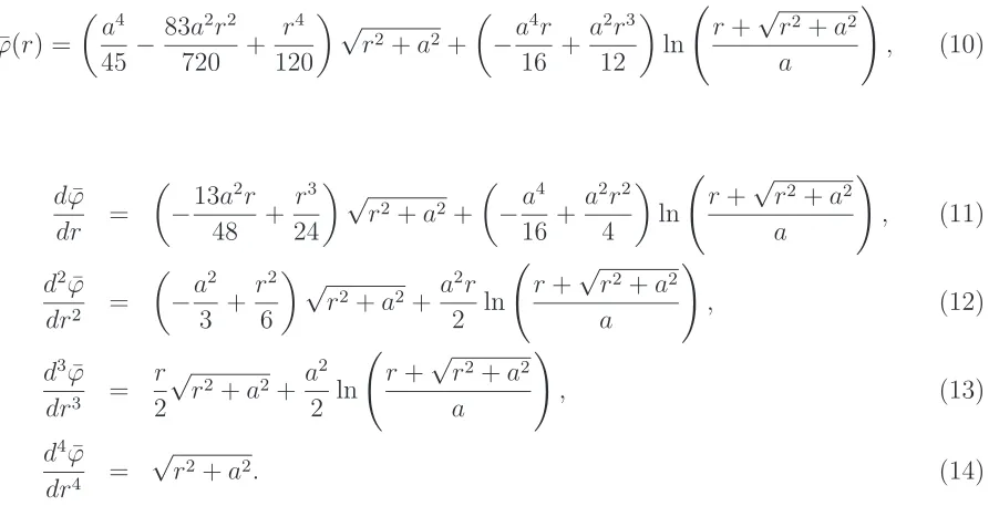
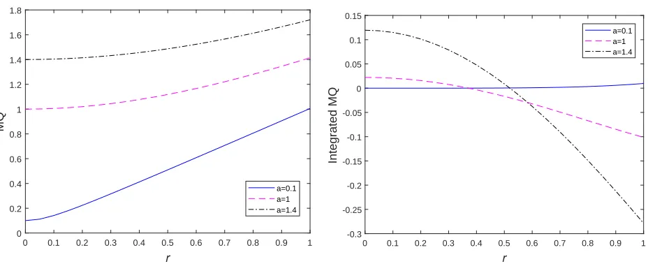
Figure 1 illustrates the shape of the MQ (2) and the integrated MQ (10) for several values of
the MQ width. It was shown in [33] that the integrated MQ approaches a large constant as
1/aapproaches zero. Both DRBFs and IRBFs are implemented in this work. For simplicity
of notation, expression (1) is now used for the two approaches, where functionϕ(r) is taken
in the form of (2) for DRBFs and in the form of (10) for IRBFs. We introduce the concept
of order for IRBF. An IRBF is said to be of order α if its (original) RBF is integrated α
times. For function ϕ defined in (10), one has α = 4. As shown in [33], this IRBF is a
conditionally positive definite function of order (α+ 2)/2 = 3 and from a theoretical point
of view, one needs to add to the interpolant a polynomial whose order is less by 1 (i.e. 2) to
acquire an invertible interpolation matrix. However, from numerical experiments reported,
to our best knowledge, a singular interpolation matrix was never observed when the IRBF
approximations were not augmented with polynomial terms. Furthermore, the addition of a
polynomial did not lead to any significant improvement in the solution accuracy at relatively
coarse disretisations.
An effective way to compute derivatives of function ϕ with respect to x and y on RHS of
(3)-(5) (k = {1,2,3,4}, m = n = 2) is to express them in terms of derivatives of ϕ with
pure derivatives with respect to x together with cross derivatives are given below ∂ϕ ∂x = dϕ dr ∂r
∂x, (15)
∂2ϕ
∂x2 =
dϕ dr
∂2r
∂x2 +
d2ϕ
dr2 ∂r ∂x 2 , (16)
∂3ϕ
∂x3 =
dϕ dr
∂3r
∂x3 + 3
d2ϕ
dr2
∂r ∂x
∂2r
∂x2 +
d3ϕ
dr3 ∂r ∂x 3 , (17)
∂4ϕ
∂x4 =
dϕ dr
∂4r
∂x4 +
d2ϕ
dr2
"
4∂r
∂x ∂3r
∂x3 + 3
∂2r
∂x2
2#
+ 6d 3ϕ dr3 ∂r ∂x 2
∂2r
∂x2 +
d4ϕ
dr4 ∂r ∂x 4 ,(18)
∂4ϕ
∂x2∂y2 =
dϕ dr
∂4r
∂x2∂y2 +
d2ϕ
dr2
"
∂2r
∂x2
∂2r
∂y2 + 2
∂2r
∂x∂y
2
+ 2∂r
∂x ∂3r
∂x∂y2 + 2
∂r ∂y
∂3r
∂x2∂y
#
+
d3ϕ
dr3
"
∂2r
∂y2
∂r ∂x
2
+ 4∂r
∂x ∂r ∂y
∂2r
∂x∂y + ∂2r
∂x2 ∂r ∂y 2# +d 4ϕ dr4 ∂r ∂x 2 ∂r ∂y 2 . (19) Since
r=kx−xjk=
q
(x−xj)2+ (y−yj)2, (20)
expressions for computing pure and cross derivatives of r on RHS of (15)-(19) are given by
∂r ∂x =
x−xj
r , (21)
∂2r ∂x2 =
r2−(x−xj)2
r3 , (22)
∂3r
∂x3 = −
3(x−xj) [r2−(x−xj)2]
r5 , (23)
∂4r
∂x4 = −
3 [r2−(x−x
j)2] [r2−5(x−xj)2]
r7 , (24)
∂2r
∂x∂y = −
(x−xj)(y−yj)
r3 , (25)
∂3r
∂x∂y2 =
(x−xj) [−(x−xj)2+ 2(y−yj)2]
r5 , (26)
∂3r
∂x2∂y =
(y−yj) [−(y−yj)2+ 2(x−xj)2]
r5 , (27)
∂4r
∂x2∂y2 = 2
r3 −
15(x−xj)2(y−yj)2
The limits of derivatives of function ϕ when r→0 are
∂ϕ ∂x →0,
∂2ϕ
∂x2 → 1
a, ∂3ϕ
∂x3 →0,
∂4ϕ
∂x4 → − 3
a3, (29)
∂ϕ ∂y →0,
∂2ϕ
∂y2 → 1
a, ∂3ϕ
∂y3 →0,
∂4ϕ
∂y4 → − 3
a3, (30)
∂4ϕ
∂x2∂y2 → − 1
a3, (31)
for DRBF and
∂ϕ ∂x →0,
∂2ϕ
∂x2 → −
a3 3 ,
∂3ϕ
∂x3 →0,
∂4ϕ
∂x4 →a, (32)
∂ϕ ∂y →0,
∂2ϕ
∂y2 → −
a3 3 ,
∂3ϕ
∂y3 →0,
∂4ϕ
∂y4 →a, (33)
∂4ϕ
∂x2∂y2 →
a
3, (34)
for IRBF. It is straightforward to obtain results (29), (30), (32) and (33). For (31) and
(34), one may need to replace the biharmonic operator with Laplace ones, and the detailed
process is described in Appendix.
As discussed early, the quality of approximations by the MQs is dependent on both their
spacing and width. For an easy interpretation, the MQ width a is expressed in terms of a
typical distance from the MQ centre to its neighbours, denoted by h, as
a=βh, (35)
where β is a constant that can run from a small to large positive value. For a given node
distribution, the value of h can be determined. The advantage of (35) lies in its simplicity
with β being a dimensionless quantity.
For the node refinement (scheme resolution), the value of his reduced. In practice, the RBF
width is then chosen to be smaller by, for example, keeping β fixed. It was shown in [21],
this common practice may lead to the issue of stagnation errors (i.e. failure of convergence
in the h→0 limit), which can be overcome by adding polynomial terms to the interpolant
h), one can change β to improve the RBF approximations. In this case, it is expected that
the addition of polynomial terms will not affect much the solution accuracy.
In this study, we focus on investigating the effects of β on the solution accuracy for a given
grid size. A wide range of β is explored by using the extended precision approach. Grid
refinements are also studied; however, only relatively coarse grids are considered, for which
the formula (35) can be applied without causing stagnation errors. It will be shown later that
the simple formula (35) can produce results that are very close to the ones corresponding to
the best values of β over a range of grid sizes.
Numerical experiments indicate that IRBFs lead to matrices of higher condition numbers
than DRBFs. For a smooth function, accurate approximations by the former may thus
occur earlier as β increases. In this regard, the comparison of accuracy between DRBFs and
IRBFs should be made over a wide range of β rather than at its some particular values.
For the presented numerical examples, in comparing the two RBF methods, a range of β is
considered as wide as possible.
3
IRBF Hermite-based method: global scheme
Consider a differential problem
Lu(x) =b(x), x∈Ω, (36)
Bu(x) =s(x), x∈Γ, (37)
where Ω and Γ are a bounded domain and its boundary, L and B some linear differential
operators, and b and s given functions. Let N be the total number of nodes and Nb the
number of boundary nodes (Nb < N). The field variable is approximated as
u(x) = Nb
X
j=1
wjBxjϕ(kx−xjk) + N
X
j=Nb+1
wjLxjϕ(kx−xjk) + M
X
k=1
where ϕ is given by (10) for IRBFs and (2) for DRBFs, the notations Lxj and Bxj mean
that L and B act onϕ considered as a function of the variablexj, and {pk(x)}Mk=1 is a basis
for theM-dimensional space (Qd
m) of alld-variate polynomials that have degree less than or equal to m. The degree of the additional polynomial in (38) is dependent on the form ofϕ
employed, for example, m = 2 for (10) and m= 0 for (2) as shown in Section 2. To account
for the addition of polynomial terms, the following extra constraints are imposed
Nb
X
j=1
wjBxpk(x)|x=xj + N
X
j=Nb+1
wjLxpk(x)|x=xj = 0, k = 1,2, . . . , M. (39)
Substitution of (38) into (37) and (36) yield
Nb
X
j=1
wjBxBxjϕ(kx−xjk) + N
X
j=Nb+1
wjBxLxjϕ(kx−xjk) + M
X
k=1
vkBxpk(x) =s(x), (40)
Nb
X
j=1
wjLxBxjϕ(kx−xjk) + N
X
j=Nb+1
wjLxLxjϕ(kx−xjk) + M
X
k=1
vkLxpk(x) =b(x). (41)
Collocation of (40) at the boundary points and of (41) at the interior grid nodes, together
with (39), result in a set of (N +M) algebraic equations for (N +M) unknowns, namely
{wj}Nj=1 and {vk}Mk=1, in which the system matrix is symmetric.
When the augmented polynomial is excluded from the RBF approximations, equations (40),
(41) and (39) reduce to
Nb
X
j=1
wjBxBxjϕ(kx−xjk) + N
X
j=Nb+1
wjBxLxjϕ(kx−xjk) =s(x), (42)
Nb
X
j=1
wjLxBxjϕ(kx−xjk) + N
X
j=Nb+1
wjLxLxjϕ(kx−xjk) = b(x), (43)
3.1
ODEs
We apply the methods to the following second-order ODE d2u/dx2 =−4π2sin(2πx), 0≤
x ≤ 1, subject to Dirichlet boundary conditions. The exact solution can be verified to be
ue(x) = sin(2πx).
Equations (40), (41) and (39) take the form
2
X
j=1
wjϕ(kx−xjk) + N
X
j=3
wj
d2ϕ(kx−x
jk)
dx2 j + 3 X k=1
vkpk(x) = sin(2πx), (44)
2
X
j=1
wj
d2ϕ(kx−x
jk)
dx2 +
N
X
j=3
wj
d4ϕ(kx−x
jk)
dx2dx2
j + 3 X k=1 vk
d2p
k(x)
dx2 =−4π
2sin(2πx), (45)
2
X
j=1
wjpk(xj) + N
X
j=3
wj
d2p
k(xj)
dx2 = 0, k ={1,2,3}. (46)
When the RBF approximations are not augmented with the polynomial terms, the above
equations become
2
X
j=1
wjϕ(kx−xjk) + N
X
j=3
wj
d2ϕ(kx−x
jk)
dx2
j
= sin(2πx), (47)
2
X
j=1
wj
d2ϕ(kx−x
jk)
dx2 +
N
X
j=3
wj
d4ϕ(kx−x
jk)
dx2dx2
j
=−4π2sin(2πx). (48)
We first compare the numerical performance of (44)-(46) and (47)-(48). The problem domain
is discretised using a set of uniformly distributed points. We take h in (35) as the grid size.
In the global scheme, the RBF approximations involve all nodes and therefore their matrix
condition number is expected to grow rapidly. Values of β here should be chosen to be
relatively small. The IRBF and DRBF results concerning the relative L2 error, denoted by
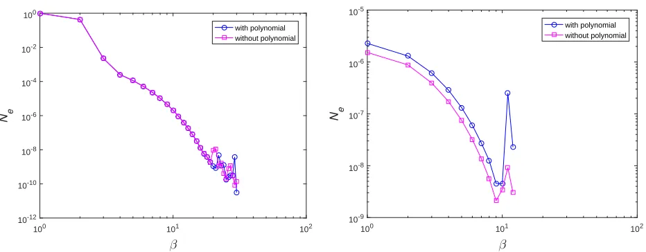
Ne, against the RBF width, displayed through β, are depicted in Figure 2, showing that
the IRBF/DRBF solutions of the two systems (i.e. (44)-(46) and (47)-(48)) have similar
behaviour. However, for IRBFs, the one without the augmented polynomial is slightly more
accurate. It appears that adding polynomial terms to the interpolants for the case of a fixed
h does not lead an improvement in accuracy. For both cases (i.e. with and without the
of the RBF width. These observations are consistent with remarks of other computational
works in the RBF literature.
In Figure 3, results by the IRBF and DRBF Hermite-based methods are compared together
for a given grid size. It can be seen that the former is generally more accurate than the latter
over a wide range of β. As β increases, the computed errors of the two methods fluctuate
due to their higher matrix condition numbers. Several algorithms to extend the working
range of the RBF width have been proposed in the literature (see, e.g. [15-19,37]). In this
work, we employ the extended precision approach. Our programs are written in Matlab
with function vpa being utilised to increase the number of significant figures from 16 to 50.
As shown in Figure 3, the calculation is now stable over the full range of the RBF width.
Results obtained indicate that the use of IRBFs leads to a significantly improved accuracy
from a small to large RBF width. The best accuracy by the two methods corresponds to
similar values of β.
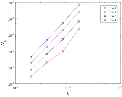
Figure 4 displays the effects of the grid size on the solution accuracy by the proposed global
Hermite-based method for several values of β. The domain is represented by uniform grids,
{101,111,· · · ,1001}. A relation between Ne and h in the log-log scale is fitted by a linear
function with its slope being regarded as an average rate of convergence. The IRBF solution
converges as O(h2.83) for β = 1, O(h2.96) for β = 3 and O(h2.90) for β = 5. Highly accurate
results are obtained; the relative L2 error is reduced to O(10−10) for β = 5. Also, constant
values of β produce similar rates of convergence; larger β corresponds to a higher level of
accuracy. These simple behaviours provide some useful guidance on how to choose the RBF
width in practical applications.
3.2
PDEs
We apply the methods to Poisson equation with its driving functionb=−2π2sin(πx) sin(πy)
and 0 ≤ x, y ≤ 1. The exact solution can be verified to be ue(x, y) = sin(πx) sin(πy) from
For Poisson equation, Lx and Lxj take the form
Lx = ∂
2
∂x2 +
∂2
∂y2, (49)
Lxj = ∂
2 ∂x2 j + ∂ 2 ∂y2 j . (50)
Since x and xj can be interchanged in defining the input r of MQ, one has
LxLxj =
∂2
∂x2 +
∂2 ∂y2 ∂2 ∂x2 j + ∂ 2 ∂y2 j , = ∂ 4
∂x4 + 2
∂4
∂x2∂y2 +
∂4
∂y4 =
∂4
∂x4
j
+ 2 ∂ 4
∂x2
j∂yj2 + ∂
4
∂y4
j
. (51)
We employ 4 set of unstructured nodes to represent the problem domain (Figure 5). The MQ
width is defined here by assuming that the nodes are of uniform distribution; the distance
h in (35) is chosen as the equivalent grid size (i.e. h = 1/(√N −1)). Figure 6 shows the
solution accuracy Ne versus the grid size h for some constant values of β. Similar remarks
to ODEs can be made here. It can be seen that highly accurate results are obtained. The
relative L2 error is reduced to O(10−7) for β = 4. As β increases, the level of accuracy is
clearly improved; however, their average rates are only about 3, e.g. 3.51 forβ = 1, 3.45 for
[image:12.612.160.469.187.255.2]β = 2, 3.22 for β= 3, and 3.10 for β = 4, probably due to the use of unstructured nodes. In
Figure 6, for large β, local rates/slopes are observed to vary with the grid size. Since global
approximations result in full matrices, their computations can be very expensive. The global
schemes are thus not suitable for large-scale applications. There is a need for having local
schemes, which is discussed next.
4
IRBF Hermite-based method: local scheme
In a local version, only neighbouring nodes are activated for the approximation at a point.
Consider a stencil associated with nodei. For the Hermite type, some nodes on the stencil are
selected to include information about ODE/PDE (Lu = b, L a linear differential operator,
special nodes just mentioned (q < n). A function is approximated as
u(x) = n
X
j=1
wjϕ(kx−xjk) + q
X
j=1 ¯
wjL¯xjϕ(kx−¯xjk) + M
X
k=1
vkpk(x), (52)
where the notation L¯xj means that L acts on ϕ considered as a function of x¯
j, {¯xj}qj=1
is a subset of {xj}nj=1, and {pk(x)}Mk=1 is a basis for the M-dimensional space (
Qd
m) of all
d-variate polynomials that have degree less than or equal to m. To account for the addition
of polynomial terms, the following extra constraints are imposed
n
X
j=1
wjpk(xj) + q
X
j=1 ¯
wjLxpk(x)|x=¯xj = 0, k = 1,2, . . . , M. (53)
Unlike Lagrange interpolation (function values only), expression (52) contains q extra
coef-ficients (i.e. {w¯j}qj=1) that allow for the process of converting the RBF coefficient space into
the physical space to take the form
u(x1) ...
u(xn)
Lxu(¯x 1) .. .
Lxu(¯x q) 0 ... 0 =
C11 C12 C13
C21 C22 C23
C31 C32 C33
w1 ... wn ¯ w1 .. . ¯ wq v1 ... vM , (54)
where the first nequations are for function values, the next qequations for derivative values
(i.e. ODE/PDE), the last M equations for the extra constraints to account for the addition
by C, and
C11
ij = ϕ(kxi−xjk), 1≤i≤n, 1≤j ≤n, (55)
C12
ij = L ¯ xjϕ(
kxi−¯xjk), 1≤i≤n, 1≤j ≤q, (56)
C13
ij = pj(xi), 1≤i≤n, 1≤j ≤M, (57)
C21
ij = L
xϕ(kx−x
jk)x=¯xi, 1≤i≤q, 1≤j ≤n, (58)
C22
ij = L
xL¯xjϕ(
kx−¯xjk)x=¯xi, 1≤i≤q, 1≤j ≤q, (59)
C23
ij = Lxpj(x)|x=x¯i, 1≤i≤q, 1≤j ≤M, (60)
C31
ij = pi(xj), 1≤i≤M, 1≤j ≤n, (61)
C32
ij = L xp
i(x)|x=x¯j, 1≤i≤M, 1≤j ≤q, (62)
C33
ij = 0, 1≤i≤M, 1≤j ≤M. (63)
When the RBF approximations are not augmented with the polynomial terms, the conversion
system reduces to
u(x1) ...
u(xn)
Lxu(¯x 1) ...
Lxu(x¯ q) =
C11 C12
C21 C22
w1 ... wn ¯ w1 ... ¯ wq , (64)
It can be seen that C is a symmetric matrix of dimensions [n +q +M, n+q +M] if the
polynomial terms are included and of dimensions [n+q, n+q] if the polynomial terms are
excluded. Making use of (54) and (64), a function and its derivatives at a point on the stencil
can be expressed in terms of function values at {xj}nj=1, which are nodal unknowns to be
found, and derivative values at {¯xj}qj=1, which can be derived from the ODE/PDE.
By collocating the ODE/PDE at the interior grid nodes, and then replacing the obtained
nodal derivative values with nodal variable values on their associated stencils, the ODE/PDE
is transformed into a set of algebraic equations, which can be solved for the values of u at
4.1
ODEs
We apply the methods to the following second-order ODE
d2u/dx2 = exp(−40x) (1500 sin(10x)−800 cos(10x)), 0≤x≤1,
subject to Dirichlet boundary conditions. The exact solution can be verified to be ue(x) =
sin(10x) exp(−40x). The domain is represented by sets of equi-spaced nodes. A stencil
associated with nodexi is proposed to have 3 nodes. We take the distancehas the grid size.
In contrast to the global approximation case, the value of β here can be chosen to be much
larger.
Figure 7 shows the effects of β on the solution accuracy Ne. Results by the DRBF
Hermite-based method are also included. For both methods, their systems are tri-diagonal and of
the same dimensions. It can be seen that IRBF outperforms DRBF over a wide range of β.
As β increases, the RBF approximations can be more accurate but its interpolation matrix
condition number also grows quickly, making the computed error Ne fluctuating at large
values of β. One can bypass this issue by using extended precision in computation. In [37],
numerical investigations indicated that the condition number of the conversion matrix grows
much faster than that of the final system matrix. Here, we only employ extended precision for
constructing and inverting small conversion matrices (other computational parts including
the solving of the final system of equations are conducted using double precision). The
obtained results are also depicted in Figure 7. At low values of β, where the matrix is
not ill-conditioned, double and extended precision basically yield the same errors. At large
values of β, by extending the calculation precision, fluctuations in the computed error are
eliminated.
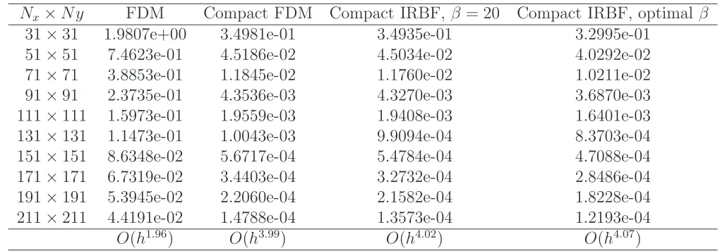
Table 1 displays the computed solutions by several numerical methods. When compared
to the classical central difference scheme, the compact approximations produce much more
accurate results. Both compact FD [38] and IRBF methods are able to yield high rates
of convergence (about fourth-order accuracy). To this problem, since its exact solution is
included in the table, which show that (i) the RBF accuracy can be further improved by
varying β; and (ii) the simple formula (35) can work well for relatively-coarse grids.
4.2
PDEs
Like the global version, the present local methods are also meshless. However, our attention
will be focused on the case of using Cartesian grid to represent the problem domain. The
main reason for us to pursue this kind of discretisation lies in its economic pre-processing,
easy implementation and its ability to also work with non-rectangular domains.
For 2D problems, a stencil associated with node xi is proposed to have 9 nodes
x3 x6 x9
x2 x5 x8
x1 x4 x7
(65)
where the fifth node (i.e. x5) is a node i in a global numbering. Four nodes 2, 4, 6 and 8
(i.e. nodes nearer to the stencil centre) are selected to include the PDE information.
For a stencil associated with an interior node that is near an irregular boundary (e.g. curved
boundary), it is proposed that the stencil consists of regular and irregular nodes (Figure 10).
Regular nodes are simply the intersection points of the stencil grid lines, while irregular nodes
are generated from the intersection of the boundary and the stencil grid lines. As a result,
for boundary stencils, the number of nodes are typically greater than 9. The imposition of
information about PDE is also implemented at side nodes on the horizontal and vertical grid
lines (i.e. 4 nodes).
4.2.1 Poisson equation
A PDE to be employed is Poisson equation, where its driving function and Dirichlet boundary
is chosen (Figure 11).
The effects of the MQ width on the solution accuracy by the IRBF and DRBF
Hermite-based methods are displayed in Figure 8 for rectangular domain and in Figure 12 for
non-rectangular domain. It can be seen that the IRBF solutions are generally more accurate
than DRBF ones over a wide range of β. At large values of β, as expected, there are
some fluctuations in the computed error Ne. To make the calculation stable, we employ
extended precision in forming the conversion matrix and computing its inverse. Since other
computational parts are carried out with double precision, a full range of β is explored with
a reasonable computational cost. With extended precision, as shown in the two figures,
fluctuations no longer occur in the computed error at large values of β.
In Figure 9, results by the compact IRBF, central difference and compact finite difference
[38] methods are displayed. Similar to second-order ODEs, the compact approximations
for PDEs outperform those based on the central differences. The compact IRBF and FD
methods yield high rates of convergence (about fourth-order accuracy). Exploiting the exact
solution, the best values of β can be found. It can be seen that the use of a fixed β for
relatively coarse grids can lead to results that are very close to the ones corresponding to
the best values ofβ. For non-rectangular domains, the problem domain is simply embedded
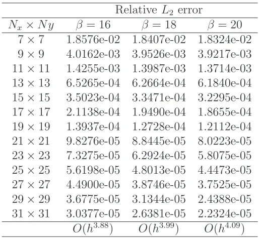
in a rectangle that is discretised using Cartesian grids of 7×7,9×9,· · · ,31×31. Table
2 displays the results obtained by the compact IRBF scheme. The solution converges as
O(h3.88) for β = 16, O(h3.99) forβ = 18 and O(h4.09) forβ = 20.
4.2.2 Convection-diffusion equation
We test the proposed local method with the following steady-state convection-diffusion
equa-tion and boundary condiequa-tions
∂2u
∂x2 +
∂2u
∂y2 −Pe
∂u
u(x,0) = u(x,1) = 0, 0≤x≤1, (67)
u(0, y) = sin(πy), u(1, y) = 2 sin(πy), 0≤y≤1, (68)
where Pe is the P´eclet number. The exact solution to this problem is given by
ue(x, y) = exp(Pex/2) sin(πy) [2 exp(−Pe/2) sinh(σx) + sinh(σ(1−x))]/sinh(σ), (69)
where σ = pπ2+P2
e/4. As Pe increases, the boundary layer will be formed. Its gradient becomes very steep at large Pe values, presenting a great challenge for any numerical
sim-ulation. We simply employ uniform grids to represent the problem domain. It is observed
that the optimal RBF width occurs earlier with respect to the RBF width whenPeincreases
from 10 to 100 (Figure 13). In contrast to problems whose solutions are smooth, the most
accurate approximation for convection-dominated problems takes place at relatively-low
val-ues of the RBF width, where the RBF system is known to be stable. Note that all smooth
curves depicted here are obtained with double-precision computations. By simply taking
β ={10,8,6,4} for Pe ={10,20,40,80}, respectively, a fast rate of convergence (i.e. about
4) is achieved (Figure 14). Figure 15 displays the present RBF solutions for several Pe
val-ues. It can be seen that they are all captured very well. At high Pe values, there are no
oscillations in the solution near the boundary layer.
5
Concluding remarks
In this study, we have introduced integrated RBFs into the Hermite interpolation method for
the numerical solution of ODEs/PDEs. Its main purpose is to yield a new strong (collocation)
form of IRBF whose interpolation matrices are symmetric and non-singular. Several schemes
based on global and local approximations for rectangular and non-rectangular domains are
presented. The extended precision approach is utilised to extend the working range of the
IRBF width for a given grid size; numerical examples show an improvement in accuracy
achieved over conventional compact IRBF Hermite-based methods. The local version is a
features, including (i) sparse system matrix; (ii) fast convergence rate; and (iii) its ability
to also work with large values of the RBF width with a relatively low computational cost.
Highly accurate results are obtained using relatively coarse grids.
Appendix
The following equation is utilised to derive the limit of the fourth-order cross derivative of
function ϕ as r→0
∇4ϕ =∇2∇2ϕ, (70)
or
∂4ϕ
∂x4 + 2
∂4ϕ
∂x2∂y2 +
∂4ϕ
∂y4 =
∂2
∂x2 +
∂2
∂y2
∂2ϕ
∂x2 +
∂2ϕ
∂y2
. (71)
Taking into account
∂r ∂x 2 + ∂r ∂y 2
= 1, ∂
2r
∂x2 +
∂2r
∂y2 = 1
r, (72)
the RHS of (71) can be rewritten in terms of derivatives of ϕ with respect toronly, and the
equation becomes
∂4ϕ
∂x4 + 2
∂4ϕ
∂x2∂y2 +
∂4ϕ
∂y4 =
d4ϕ
dr4 + 2
r d3ϕ
dr3 − 1
r2
d2ϕ
dr2 + 1
r3
dϕ
dr, (73)
from there, as r→0, one can acquire
∂4ϕ
∂x2∂y2 → − 1
a3 for DRBF,
∂4ϕ
∂x2∂y2 →
a
3 for IRBF.
References
1. C.A. Micchelli, Interpolation of scattered data: distance matrices and conditionally
positive definite functions, Constructive Approximation 2, (1986), 11-22.
2. W.R. Madych, Miscellaneous error bounds for multiquadric and related interpolators,
3. E.J. Kansa, Multiquadrics - A scattered data approximation scheme with applications
to computational fluid-dynamics - II. Solutions to parabolic, hyperbolic and elliptic
partial differential equations, Computers and Mathematics with Applications 19(8/9),
(1990), 147-161.
4. E.J. Kansa, H. Power, G.E. Fasshauer and L. Ling, A volumetric integral radial
ba-sis function method for time-dependent partial differential equations: I. Formulation,
Engineering Analysis with Boundary Elements 28, (2004), 1191-1206.
5. N. Mai-Duy and R.I. Tanner, Computing non-Newtonian fluid flow with radial basis
function networks, Int. J. Numer. Meth. Fluids 48, (2005), 1309-1336.
6. B. Sarler, A radial basis function collocation approach in computational fluid dynamics,
CMES: Computer Modeling in Engineering & Sciences 7(2), (2005), 185-194.
7. M. Li, T. Jiang and Y.C. Hon, A meshless method based on RBFs method for
nonho-mogeneous backward heat conduction problem, Engineering Analysis with Boundary
Elements 34(9), (2010), 785-792.
8. C.-M. Fan, C.-S. Chien, H.-F. Chan and C.-L. Chiu, The local RBF collocation method
for solving the double-diffusive natural convection in fluid-saturated porous media,
International Journal of Heat and Mass Transfer 57(2), (2013), 500-503.
9. M. Li, W. Chen and C.S. Chen, The localized RBFs collocation methods for solving
high dimensional PDEs, Engineering Analysis with Boundary Elements 37(10), (2013),
1300-1304.
10. D. Stevens, H. Power and K.A. Cliffe, A solution to linear elasticity using locally
sup-ported RBF collocation in a generalised finite-difference mode, Engineering Analysis
with Boundary Elements 37(1), (2013), 32-41.
11. F.J. Mohammed, D. Ngo-Cong, D.V. Strunin, N. Mai-Duy and T. Tran-Cong,
Mod-elling dispersion in laminar and turbulent flows in an open channel based on centre
manifolds using 1D-IRBFN method, Applied Mathematical Modelling, 38(14), (2014),
12. M. Dehghan and V. Mohammadi, The numerical solution of FokkerPlanck equation
with radial basis functions (RBFs) based on the meshless technique of Kansa’s
ap-proach and Galerkin method, Engineering Analysis with Boundary Elements 47, (2014),
38-63.
13. A. Vidal, A.J. Kassab and E.A. Divo, A direct velocity-pressure coupling Meshless
al-gorithm for incompressible fluid flow simulations, Engineering Analysis with Boundary
Elements 72, (2016), 1-10.
14. H. Zheng, C. Zhang, Y. Wang, J. Sladek and V. Sladek, A meshfree local RBF
colloca-tion method for anti-plane transverse elastic wave propagacolloca-tion analysis in 2D phononic
crystals, Journal of Computational Physics 305, (2016), 997-1014.
15. B. Fornberg and G. Wright, Stable computation of multiquadric interpolants for all
values of the shape parameter, Computers and Mathematics with Applications 48(5-6),
(2004), 853-867.
16. G.B. Wright and B. Fornberg, Scattered node compact finite difference-type formulas
generated from radial basis functions, Journal of Computational Physics 212(1), (2006),
99-123.
17. C.-S. Huang, C.-F. Lee and A.H.-D. Cheng, Error estimate, optimal shape factor, and
high precision computation of multiquadric collocation method, Engineering Analysis
with Boundary Elements 31(7), (2007), 614-623.
18. C.-S. Huang, H.-D. Yen and A.H.-D. Cheng, On the increasingly flat radial basis
function and optimal shape parameter for the solution of elliptic PDEs, Engineering
Analysis with Boundary Elements 34(9), (2010), 802-809.
19. B. Fornberg, E. Larsson and N. Flyer, Stable computations with Gaussian radial basis
functions, SIAM Journal on Scientific Computing 33(2), (2011), 869-892.
20. J. Rashidinia, G.E. Fasshauer and M. Khasi, A stable method for the evaluation of
Gaussian radial basis function solutions of interpolation and collocation problems,
21. N. Flyer, B. Fornberg, V. Bayona and G.A. Barnett, On the role of polynomials in
RBF-FD approximations: I. Interpolation and accuracy, Journal of Computational
Physics 321, (2016), 21-38.
22. Y.C. Hon and R. Schaback, On unsymmetric collocation by radial basis functions,
Applied Mathematics and Computation 119(23), (2001), 177-186.
23. R.L. Hardy, Research results in the application of multiquadric equations to surveying
and mapping problems, Survg Mapp. 35, (1975), 321332.
24. Z. Wu, Hermite-Birkhoff interpolation of scattered data by radial basis functions,
Ap-proximation Theory and its Applications 8(2), (1992), 1-10.
25. X. Sun, Scattered Hermite interpolation using radial basis functions, Linear Algebra
and its Applications 207, (1994), 135-146.
26. G.E. Fasshauer, “Solving partial differential equations by collocation with radial basis
functions,” in Surface Fitting and Multiresolution Methods, A. LeMhaut, C. Rabut and
L.L. Schumaker (Editors), Vanderbilt University Press, Nashville, 1997, p. 131-138.
27. H. Power and V. Barraco, A comparison analysis between unsymmetric and symmetric
radial basis function collocation methods for the numerical solution of partial
differen-tial equations, Computers and Mathematics with Applications 43, (2002), 551-583.
28. E. Larsson and B. Fornberg, A numerical study of some radial basis function based
solution methods for elliptic PDEs, Computers and Mathematics with Applications
46, (2003), 891-902.
29. A.I. Tolstykh and D.A. Shirobokov, Using radial basis functions in a “finite difference
mode”, CMES: Computer Modeling in Engineering & Sciences 7(2), (2005), 207-222.
30. N. Mai-Duy and T. Tran-Cong, Compact local integrated-RBF approximations for
second-order elliptic differential problems, Journal of Computational Physics 230(12),
(2011), 4772-4794.
mul-32. L. Ling and M.R. Trummer, Multiquadric collocation method with integral formulation
for boundary layer problems, Computers and Mathematics with Applications 48(5-6),
(2004), 927-941.
33. S.A. Sarra, Integrated multiquadric radial basis function approximation methods,
Com-puters and Mathematics with Applications 51(8), (2006), 1283-1296.
34. C. Shu and Y.L. Wu, Integrated radial basis functions-based differential quadrature
method and its performance, International Journal for Numerical Methods in Fluids
53(6), (2007), 969-984.
35. C.S. Chen, C.M. Fan and P.H. Wen, The method of approximated particular
solu-tions for solving certain partial differential equasolu-tions, Numerical Methods for Partial
Differential Equations 28(2), (2010), 506-522.
36. N. Mai-Duy and T. Tran-Cong, A compact five-point stencil based on integrated
RBFs for 2D second-order differential problems, Journal of Computational Physics
235, (2013), 302-321.
37. N. Mai-Duy, T.T.V. Le, C.M.T. Tien, D. Ngo-Cong and T. Tran-Cong, Compact
approximation stencils based on integrated flat radial basis functions, Engineering
Analysis with Boundary Elements 74, (2017), 79-87.
38. L. Collatz, The Numerical Treatment of Differential Equations, Springer-Verlag, Berlin,
Table 1: ODE, double precision: Relative L2 errors of the computed solutions. Compact approximations outperform those based on the classical central differences. Both compact FD and IRBF schemes are able to yield high rates of convergence with respect to grid refinement. Given an analytic form of the solutionu, the best values ofβ can be determined numerically and their corresponding solutions are also included for comparison purposes.
Nx×Ny FDM Compact FDM Compact IRBF, β= 20 Compact IRBF, optimal β
31×31 1.9807e+00 3.4981e-01 3.4935e-01 3.2995e-01
51×51 7.4623e-01 4.5186e-02 4.5034e-02 4.0292e-02
71×71 3.8853e-01 1.1845e-02 1.1760e-02 1.0211e-02
91×91 2.3735e-01 4.3536e-03 4.3270e-03 3.6870e-03
111×111 1.5973e-01 1.9559e-03 1.9408e-03 1.6401e-03
131×131 1.1473e-01 1.0043e-03 9.9094e-04 8.3703e-04
151×151 8.6348e-02 5.6717e-04 5.4784e-04 4.7088e-04
171×171 6.7319e-02 3.4403e-04 3.2732e-04 2.8486e-04
191×191 5.3945e-02 2.2060e-04 2.1582e-04 1.8228e-04
211×211 4.4191e-02 1.4788e-04 1.3573e-04 1.2193e-04
Table 2: PDE, non-rectangular domain, double precision: Grid convergence by the local IRBF Hermite-based scheme for several RBF widths .
Relative L2 error
Nx×Ny β= 16 β = 18 β = 20 7×7 1.8576e-02 1.8407e-02 1.8324e-02 9×9 4.0162e-03 3.9526e-03 3.9217e-03 11×11 1.4255e-03 1.3987e-03 1.3714e-03 13×13 6.5265e-04 6.2664e-04 6.1840e-04 15×15 3.5023e-04 3.3471e-04 3.2295e-04 17×17 2.1138e-04 1.9490e-04 1.8655e-04 19×19 1.3937e-04 1.2728e-04 1.2112e-04 21×21 9.8276e-05 8.8445e-05 8.0223e-05 23×23 7.3275e-05 6.2924e-05 5.8075e-05 25×25 5.6198e-05 4.8013e-05 4.4473e-05 27×27 4.4900e-05 3.8746e-05 3.7525e-05 29×29 3.6775e-05 3.1344e-05 2.4388e-05 31×31 3.0377e-05 2.6381e-05 2.2324e-05
0 0.1 0.2 0.3 0.4 0.5 0.6 0.7 0.8 0.9 1
r
0 0.2 0.4 0.6 0.8 1 1.2 1.4 1.6 1.8
MQ
a=0.1 a=1 a=1.4
0 0.1 0.2 0.3 0.4 0.5 0.6 0.7 0.8 0.9 1
r
-0.3 -0.25 -0.2 -0.15 -0.1 -0.05 0 0.05 0.1 0.15
Integrated MQ
[image:26.612.87.551.26.215.2]a=0.1 a=1 a=1.4
100 101 102
β
10-12 10-10
10-8 10-6 10-4 10-2 100
N e
with polynomial without polynomial
100 101 102
β
10-9 10-8
10-7 10-6 10-5
N e
[image:27.612.84.550.27.209.2]with polynomial without polynomial
100 101 102
β
10-20
10-15
10-10
10-5
100
N
e [image:28.612.112.507.27.340.2]DRBF, double precision DRBF, extended precision IRBF, double precision IRBF, extended precision
10-3 10-2
h
10-10
10-9
10-8
10-7
10-6
10-5
N
e [image:29.612.112.510.28.338.2]=1 =3 =5
10-2 10-1 100
h
10-7
10-6
10-5
10-4
10-3
10-2
N
eβ = 1
β = 2
β = 3
[image:31.612.110.506.28.343.2]β = 4
100 101 102
β
10-6
10-5
10-4
10-3
10-2
10-1
100
N
e [image:32.612.110.505.29.344.2]DRBF, double precision DRBF, extended precision IRBF, double precision IRBF, extended precision
100 101 102
β
10-5
10-4
10-3
10-2
10-1
N
e [image:33.612.113.508.24.341.2]DRBF, double precision DRBF, extended precision IRBF, double precision IRBF, extended precision
10-2 10-1 100
h
10-4
10-3
10-2
10-1
100
N
eFDM
[image:34.612.110.507.31.341.2]Compact FDM Compact IRBF, =30 Compact IRBF, optimal
1
3
4
6
7
9
2
8
5
10
11
12
[image:35.612.125.507.34.475.2]boundary
0 0.1 0.2 0.3 0.4 0.5 0.6 0.7 0.8 0.9 1
x
00.1 0.2 0.3 0.4 0.5 0.6 0.7 0.8 0.9 1
y
[image:36.612.113.508.30.351.2]Interior node Boundary node
100 101 102
10-5
10-4
10-3
10-2
10-1
100
N
e [image:37.612.114.507.30.344.2]DRBF IRBF
100 101
β
10-5
10-4
10-3
10-2
10-1
100
N
eP
e=10
P
e=20
P
e=40
P
[image:38.612.112.507.24.342.2]e=100
10-2 10-1 100
h
10-6
10-5
10-4
10-3
10-2
10-1
100
N
eP e=10 P
e=20 P
e=40 P
[image:39.612.112.505.32.342.2]e=100
Figure 14: Convection-diffusion equation, double precision: Effects of the grid size on the solution accuracy for several P´eclet numbers by the proposed local Hermite-based method. Values of β used are {10, 8, 6, 4} for Pe = {10,20,40,100}, respectively. The solution converges asO(h4.24) forP
e = 10, O(h4.23) forPe= 20, O(h4.34) forPe= 40 and O(h4.61) for
Pe = 10 Pe = 20 0 1 0.5 1 1 u(x,y) 0.8 1.5 y 0.5 0.6 x 2 0.4 0.2 0 0 0 1 0.5 1 1 u(x,y) 0.8 1.5 y 0.5 0.6 x 2 0.4 0.2 0 0
Pe = 40 Pe= 100
[image:40.612.86.573.71.491.2]0 1 0.5 1 1 u(x,y) 0.8 1.5 y 0.5 0.6 x 2 0.4 0.2 0 0 0 1 0.5 1 1 u(x,y) 0.8 1.5 y 0.5 0.6 x 2 0.4 0.2 0 0