Beyond Lean: Simulation in Practice, Second Edition

(1)

Beyond Lean:

(2)

Beyond Lean: Simulation in Practice

Second Edition

©Charles R. Standridge, Ph.D. Professor of Engineering

Assistant Dean

Padnos College of Engineering and Computing Grand Valley State University

301 West Fulton Grand Rapids, MI 49504

616-331-6759 Email:[email protected]

Fax: 616-331-7215

(3)

Table of Contents Preface

Part I Introduction and Methods

1. Beyond Lean: Process and Principles 1.1 Introduction

1.2 An Industrial Application of Simulation

1.3 The Process of Validating a Future State with Models 1.4 Principles for Simulation Modeling and Experimentation 1.5 Approach

1.6 Summary

Questions for Discussion Active Learning Exercises

2. Simulation Modeling 2.1 Introduction

2.2 Elementary Modeling Constructs 2.3 Models of System Components

2.3.1 Arrivals 2.3.2 Operations 2.3.3 Routing Entities 2.3.4 Batching 2.3.5 Inventories 2.4 Summary

Problems

3. Modeling Random Quantities 3.1 Introduction

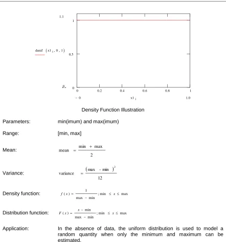
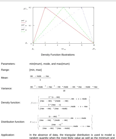
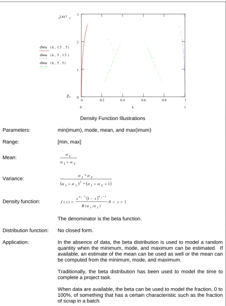
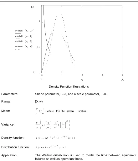
3.2 Determining a Distribution in the Absence of Data

3.2.1 Distribution Functions Used in the Absence of Data

3.2.2 Selecting Probability Distributions in the Absence of Data – An Illustration

3.3 Fitting a Distribution Function to Data 3.3.1 Some Common Data Problems

3.3.2 Distribution Functions Most Often Used in a Simulation Model

3.3.3 A Software Based Approach to Fitting a Data Set to a Distribution Function

3.4 Summary Problems

Active Learning Exercises Laboratories

(4)

4. Conducting Simulation Experiments 4.1 Introduction

4.2 Verfication and Validation 4.2.1 Verification Procedures 4.2.2 Validation Procedures

4.3 The Problem of Correlated Observations 4.4 Common Design Elements

4.4.1 Model Parameters and Their Values 4.4.2 Performance Measures

4.4.3 Streams of Random Samples

4.5 Design Elements Specific to Terminating Simulation Experiments 4.5.1 Initial Conditions

4.5.2 Replicates

4.5.3 Ending the Simulation 4.5.4 Design Summary

4.6 Examining the Results for a Single Scenario

4.6.1 Graphs, Histograms, and Summary Statistics 4.6.2 Confidence Intervals

4.6.3 Animating Model Dynamics 4.7 Comparing Scenarios

4.7.1 Comparison by Examination 4.7.2 Comparison by Statisical Analysis

4.7.2.1 A Word of Caution about Comparing Scenarios 4.8 Summary

Problems

5. The Simulation Engine 5.1 Introduction

5.2 Events and Event Graphs 5.3 Time Advance and Event Lists

5.4 Simulating the Two Workstation Model 5.5 Organizing Entities Waiting for a Resource 5.6 Random Sampling from Distribution Functions 5.7 Pseudo-Random Number Generation

(5)

Part II Basic Organizations for Systems

6. A Single Workstation 6.1 Introduction

6.2 Points Made in the Case Study 6.3 The Case Study

6.3.1 Define the Issues and Solution Objective 6.3.2 Build Models

6.3.3 Identify Root Causes and Assess Initial Alternatives 6.3.3.1 Analytic Model of a Single Workstation 6.3.3.2 Simulation Model of a Single Workstation 6.3.4 Review and Extend Previous Work

6.3.4.1 Detractors to Workstation Performance 6.4 The Case Study for Detractors

6.4.3 Assessment of the Impact of the Detractors on Part Lead Time 6.5 Summary

Problems

Application Problems

7. Serial Systems 7.1 Introduction

7.3.3 Identify Root Causes and Assess Initial Alternatives 7.3.4 Review and Extend Previous Work

7.3.5 Implement the Selected Solution and Evaluate 7.4 Summary

Problems

8. Job Shops

8.1 Introduction

(6)

Part III Lean and Beyond Manufacturing

9. Inventory Organization and Control 9.1 Introduction

9.2 Traditional Inventory Models

9.2.1 Trading off Number of Setups (Orders) for Inventory 9.2.2 Trading off Customer Service Level for Inventory 9.3 Inventory Models for Lean Manufacturing

9.3.1 Random Demand – Normally Distributed 9.3.2 Random Demand – Discrete Distributed 9.3.3 Unreliable Production – Discrete Distributed

9.3.4 Unreliable Production and Random Demand – Both Discrete Distributed 9.3.5 Production Quantities

9.3.6 Demand in a Discrete Time Period

9.3.7 Simulation Model of an Inventory Situation 9.4 Introduction to Pull Inventory Management

9.4.1 Kanban Systems: One Implementation of the Pull Philosophy 9.4.2 CONWIP Systems: A Second Implementation of the Pull Philosophy 9.4.3 POLCA: An Extension to CONWIP

Problems

10. Inventory Control Using Kanbans 10.1 Introduction

Problems

11. Cellular Manufacturing Operations 11.1 Introduction

Problems

(7)

12. Flexible Manufacturing Systems 12.1 Introduction

Problems

Application Problem

Part IV Supply Chain Logistics

13. Automated Inventory Management 13.1 Introduction

Problems

Application Problem

14. Transportation and Delivery 14.1 Introduction

Problems

Application Problem

(8)

Part V Material Handling

16. Distribution Centers and Conveyors 16.1 Introduction

16.4 Alternative Worker Assignment 16.4.1 Build Models

16.4.2 Identify Root Causes and Assess Initial Alternatives 16.4.3 Implement the Selected Solution and Evaluate 16.5 Summary

Problems

Application Problem

17. Automated Guided Vehicle Systems 17.1 Introduction

17.4 Assessment of Alternative Pickup and Dropoff Points 17.4.1 Identify Root Causes and Assess Initial Alternatives 17.4.2 Review and Extend Previous Work

Problems

Application Problem

18. Automated Storage and Retrieval 18.1 Introduction

Problems

Application Problem

Appendices

AutoMod Summary and Tutorial for the Chapter 6 Case Study

(9)

Preface

Perspective

Lean thinking, as well as associated processes and tools, have involved into a ubiquitous perspective for improving systems particularly in the manufacturing arena. With application experience has come an understanding of the boundaries of lean capabilities and the benefits of getting beyond these boundaries to further improve performance. Discrete event simulation is recognized as one beyond-the-boundaries of lean technique. Thus, the fundamental goal of this text is to show how discrete event simulation can be used in addition to lean thinking to achieve greater benefits in system improvement than with lean alone.

Realizing this goal requires learning the problems that simulation solves as well as the methods required to solve them. The problems that simulation solves are captured in a collection of case studies. These studies serve as metaphors for industrial problems that are commonly addressed using lean and simulation.

Learning simulation requires doing simulation. Thus, a case problem is associated with each case study. Each case problem is designed to be a challenging and less than straightforward extension of the case study. Thus, solving the case problem using simulation requires building on and extending the information and knowledge gleaned from the case study. In addition, questions are provided with each case problem so that it may be discussed in a way similar to the traditional discussion of case problems used in business schools, for example.

An understanding of simulation methods is prerequisite to the case studies. A simulation project process, basic simulation modeling methods, and basic simulation experimental methods are presented in the first part of the text. An overview of how a simulation model is executed on a computer is provided. A discussion of how to select a probability distribution function to model a random quantity is included. Exercises are included to provide practice in using the methods.

In addition to simulation methods, simple (algebra-level) analytic models are presented. These models are used in partnership with simulation models to better understand system behavior and help set the bounds on parameter values in simulation experiments.

The second part of the text presents application studies concerning prototypical systems: a single workstation, serial lines, and job shops. The goal of these studies is to illustrate and reinforce the use of the simulation project process as well as the basic modeling and experimental methods. The case problems in this part of the text are directly based on the case study and can be solved in a straightforward manor. This provides students the opportunity to practice the basic methods of simulation before attempting more challenging problems.

(10)

simulation results. References to more advanced simulation statistical analysis techniques are given as appropriate. Only the most basic simulation modeling methods are presented, plus extensions as needed for each particular application study.

The text is intended to help prepare those who read it to effectively perform simulation applications.

Using the Text

The text is designed to adapt to the needs of a wide range of introductory classes in simulation and production operations. Chapters 1 - 5 provide the foundation in simulation methods that every student needs and that is pre-requisite for studying the remaining chapters. Chapters 6, 7, and 8 cover basic ideas concerning how the simulation methods are used to analysis systems as well as how systems work. I would suggest that these 8 chapters be a part of every class.

A survey of simulation application areas can be accomplished by selecting chapters from parts III, IV, and V. A focus on manufacturing systems is achieved by covering chapters 9, 10, 11, and 12. A course on material handling and logistics could include chapters 13 through 18.

Compute-based activities that are a part of the problem sets can be used to help students better understand how systems operate and how simulation methods work. The case problems can be discussed in class only or a student can perform a complete analysis of the problem using simulation.

Acknowledgements

The greatest joy I have had in developing this text is to recall all of the colleagues and students with whom I have worked on simulation projects and other simulation related activities since A. Alan B. Pritsker introduced me to simulation in January 1975.

One genesis for this text came from Professor Ronald Askin. As we completed work on the text: Modeling and Analysis of Manufacturing Systems, we surmised that an entire text on the applications of simulation was needed to fully discuss the material that had been condensed into a single chapter.

Professor Jon Marvel provided invaluable advice and direction on the development of the chapter on cellular manufacturing systems.

Special thanks are due to Dr. David Heltne, retired from Shell Global Solutions. Our joint work on using simulation to address logistics and inventory management issues over much of two decades greatly influenced those areas of the text.

The masters work of several students in the School of Engineering at Grand Valley State University is reflected within the text. These include Mike Warber, Carrie Grimard, Sara Maas, and Eduardo Perez. Joel Oostdyk and Todd Frazee helped gather information that was used in this text.

(11)

Part I Introduction

This book discusses how, in a practical way, to overcome the limitations of the lean approach to transforming manufacturing systems as well as related in-plant, plant, and plant-to-customer logistics. The primary tools in this regard are algebra based mathematical models and computer-based systems simulation as well as the integration of these two. Concepts, methods, and application studies related to designing and operating such systems are presented. Emphasis is on learning how to effectively make design, planning, and operations decisions by using a model based analysis and synthesis process. This process places equal emphasis on building models and performing analyses. This first part of the book discusses this process as well as the methods required for performing each of its steps.

The beyond lean approach is introduced in chapter 1 and illustrated with an industrial application. One proven process for performing a beyond lean study is presented. Some principles that guide such studies are discussed.

Methods are considered in chapters 2 through 5: model building, the computations needed to simulate a model and experimentation with models as well as modeling time delays and other random quantities. The basic logic used in simulation models is discussed. A process by which a distribution function can be selected to represent a random quantity, in the presence or absence of data, is given. An overview of the internal operations of a simulation engine is presented.

Chapter 2 describes the most basic ways in which systems are represented in simulation models. These basic ways provide a foundation for the models that are presented in the application study chapters. The modeling of common system components: arrivals, operations, routing, batching, and inventories, is discussed.

Chapter 3 presents a discussion of how to choose a distribution function to characterize the time between arrivals, processing times, and other system components that are modeled as random variables. A computer based interactive procedure for fitting a distribution function to data is emphasized. A discussion of selecting a distribution function in the absence of data is presented.

Chapter 4 presents the design and analysis of simulation experiments. Model and experiment verification and validation are included. An approach to specifying simulation experiments is discussed. Methods, including statistical analyses, for examining simulation results are included. An overview of animation is given.

(12)

Chapter 1

Beyond Lean: Process and Principles

1.1 Introduction

The application of lean concepts to the transformation of manufacturing and other systems has become ubiquitous and is still expanding (Learnsigma, 2007). The use of lean concepts has yielded impressive results. However, there seems to be a growing recognition of the limitations of lean and for a need to overcome them, that is to build upon lean successes or in other words to get beyond lean.1 Getting beyond lean is the subject of this book.

Ferrin, Muller, and Muthler (2005) identify an important goal of any process improvement or transformation: find a correct, or at least a very good, solution that meets system design and operation requirements before implementation. Lean seems to be unable to meet this goal. As was pointed out by Marvel and Standridge (2009), a lean process does not typically validate the future state before implementation. Thus, there is no guarantee that a lean transformation will meet measurable performance objectives.

Marvel, Schaub & Weckman (2008) give one example of the consequences of not validating the future state before implementation in a case study concerning a tier-two automotive supplier. Due to poor performance of the system, a lean transformation was performed. One of the important components of the system was containers used to ship product to a number of customers. Each customer had a dedicated set of containers. The number of containers needed in the future state was estimated using a tradition lean static (average value) analysis, without taking the variability of shipping time to and from customers nor the variability in the time containers spent a customers into account. Thus, the number of containers in the future state was too low. Upon implementation, this resulted in the production system being idled due to the lack of containers. Thus, customer demand could not be met.

Standridge and Marvel (2006) describe the lean transformation of a system consisting of three processes. The second process, painting, was outsourced and performed in batches of 192 parts. Fearful of starving the third step in the process, the lean supply chain team deliberately over estimated the number of totes used to transport parts to and from the second step. In this system, totes are expensive and have a large footprint. Thus, the future state was systematically designed to be more expensive that necessary.

It seems obvious that in both these examples, the lean transformation resulted in a future state that was less than lean because it was not validated before implementation. Miller, Pawloski, and Standridge (2010) present a case study that further emphasizes this point and shows the benefits of such a validation. Marvel and Standridge (2009) suggest a modification of the lean process that includes future state validation as well as proposing that discrete event computer simulation be the primary tool for such a transformation because this tool has the following capabilities.

1. A simulation model can be analyzed using computer based experiments to assess future state performance under a variety of conditions.

2. Time is included so that dynamic changes in system behavior can be represented and assessed.

3. The behavior of individual entities such as parts, inventory levels, and material handling devices can be observed and inferences concerning their behavior made.

4. The effects of variability, both structural and random, on system performance can be evaluated.

5. The interaction effects among components can be implicitly or explicitly included.

1

(13)

The discussion in this book focuses on how to build and use models to enhance lean transformations, that is to get beyond lean or to make lean more lean. The modeling perspective used incorporates the steps required to operate the system and how these steps are connected to each other. Models include the equipment and other resources needed to perform each step as well as the decision points and decision rules that govern how each step is accomplished and is connected to other steps. These models can include the sequencing procedures, routing, and other logic that is needed for a system to effectively operate.

Computer simulation models provide information about the temporal dynamics of systems that is available from no other source. This information is necessary to determine whether a new or transformed system will perform as intended before it is put into everyday use. Simulation leads to an understanding of why a system behaves as it does. It helps in choosing from among alternative system designs and operating strategies.

When a new system is designed or an existing system substantially changed, computer simulation models are used to generate information that aids in answering questions such as the following:

1. Can the number of machines or workers performing each operation adequate or must the number be increased?

2. Will throughput targets be reached that is will the required volume of output per unit time be achieved?

3. Can routing schemes or production schedules be improved? 4. Which sequencing scheme for inputs is best?

5. What should be the work priorities of material handling devices? 6. What decision rules work best?

7. What tasks should be assigned to each worker? 8. Why did the system behave that way?

9. What would happen if we did “this” instead?

1.2 An Industrial Application of Simulation

In order to better understand what simulation is and what problems it can be used to address, consider the following industrial application, which can was used to validate the future state of a plant expansion (Standridge and Heltne, 2000). A particular plant is concerned about the capital resources needed to load and ship rail cars in a timely fashion. A major capital investment in the plant will be made but the chance for future major expansions is minimal. Thus, all additional loading facilities, called load spots, needed for the foreseeable future must be built at the current time and must be justified based on product demand forecasts.

(14)

The plant must lease rail cars to ship product to customers. Different products may require different types of rail cars, so the size of multiple rail car fleets must be estimated. In addition, the size of the plant rail yard must be determined as a function of the number of rail cars it must hold.

The model must account for customer demand for each product. Monthly demand ranges from 80% to 120% of its expected value. The expected demand for some products varies by month. In addition, each load spot must be defined by its capacity in rail cars loaded per day as well as the products it can load. Rail car travel times to customers from the plant and from the customer to the plant as well as rail car residence time at the customer site must be considered. Rail car maintenance specifications must be included.

Model logic is as follows. Each day the number of rail cars to ship is determined for each product. A rail car of the proper type waiting at the plant is assigned to the shipment. If no such rail car exists, the model simply creates a new one and the fleet size is increased by one.

(15)

Analysts formulate alternatives by changing the assignment of products to load spots, the number of load spots available, and the demand for each product. These alternatives are based, in part, on model results previously obtained.

This example shows some of the primary benefits and unique features of simulation. Unique system characteristics, such as the assignment of particular products to particular load spots, can be incorporated into models. System specific logic for assigning a shipment to a load spot is used. Various types of performance measures can be output from the model such as statistical summaries about on time shipping and time series of values about the amount of product shipped. Statistics other than the average can be estimated. For example, the size of the rail yard must accommodate the maximum number of rail cars that can be there not the average. Random and time varying quantities, such as product demand, can be easily incorporated into a model.

1.3 The Process of Validating a Future State with Models

The simulation process used throughout this book is presented in this section.

Using simulation in designing or improving a system is itself a process. We summarize these steps into five strategic process phases (Standridge and Brown-Standridge, 1994; Standridge, 1998), which are similar to those in Banks, Carson, Nelson, and Nicol (2009). The strategic phases and the tactics used in each are shown in Table 1-1.

The first strategic phase in the simulation project process is the definition of the system design or improvement issues to be resolved and the characteristics of a solution to these issues. This requires identification of the system objects and system outputs that are relevant to the problem as well as the users of the system outputs and their requirements. Alternatives thought to result in system improvement are usually proposed. The scope of the model is defined, including the specification of which elements of a system are included and which are excluded. The quantities used to measure system performance are defined. All assumptions on which the model is based are stated. All of the above items should be recorded in a document. The contents of such a document is often referred to as the conceptual model. A team of simulation analysts, system experts, and managers performs this phase.

The construction of models of the system under study is the focus of the second phase. Simulation models are constructed as described in the next chapter. If necessary to aid in the construction of the simulation model, descriptive models such as flowcharts may be built.

(16)

[image:16.612.87.529.90.428.2]

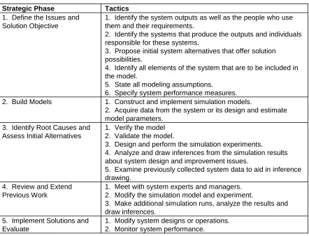
Table 1-1: Phases and Tactics of the Simulation Project Process

Strategic Phase Tactics

1. Define the Issues and Solution Objective

1. Identify the system outputs as well as the people who use them and their requirements.

2. Identify the systems that produce the outputs and individuals responsible for these systems.

3. Propose initial system alternatives that offer solution possibilities.

4. Identify all elements of the system that are to be included in the model.

5. State all modeling assumptions.

6. Specify system performance measures. 2. Build Models 1. Construct and implement simulation models.

2. Acquire data from the system or its design and estimate model parameters.

3. Identify Root Causes and Assess Initial Alternatives

1. Verify the model 2. Validate the model.

3. Design and perform the simulation experiments. 4. Analyze and draw inferences from the simulation results about system design and improvement issues.

5. Examine previously collected system data to aid in inference drawing.

4. Review and Extend Previous Work

1. Meet with system experts and managers. 2. Modify the simulation model and experiment.

3. Make additional simulation runs, analyze the results and draw inferences.

5. Implement Solutions and Evaluate

1. Modify system designs or operations. 2. Monitor system performance.

The third strategic phase involves identifying the system operating parameters, control strategies, and organizational structure that impact the issues and solution objectives identified in the first phase. Cause and effect relationships between system components are uncovered. The most basic and fundamental factors affecting the issues of interest, the root causes, are discovered. Possible solutions proposed during the first phases are tested using simulation experiments. Verification and validation are discussed in the next section as well as in Chapter 3.

Information resulting from experimentation with the simulation model is essential to the understanding of a system. Simulation experiments can be designed using standard design of experiments methods. At the same time, as many simulation experiments can be conducted as computer time and the limits on project duration allows. Thus, experiments can be replicated as needed for greater statistical precision, designed sequentially by basing future experiments on the results of preceding ones, and repeated to gather additional information needed for decision making.

(17)

sequentially. Alternative solutions may be generated using formal ways for searching a solution space such as a response surface method. In addition, system experts may suggest alternative strategies, for example alternative part routings based on the work-in-process inventory at workstations. Performing additional experiments involves modifications to the simulation model as well as using new model parameter values.

Physical experiments using the actual system or laboratory prototypes of the system may be performed to confirm the benefits of the selected system improvements.

In the fifth phase, the selected improvements are implemented and the results monitored.

The iterative nature of the simulation project process should be emphasized. At every phase, new knowledge about the system and its behavior is gained. This may lead to a need to modify the work performed at any preceding phase. For example, the act of building a model, phase 2, may lead to a greater understanding of the interaction between system components as well as to redoing phase 1 to restate the solution objectives. Analyzing the simulation results in phase 3 may point out the need for more detailed information about the system. This can lead to the inclusion of additional system components in the model as phase 2 is redone.

Sargent (2009) states that model credibility has to do with creating the confidence managers and systems experts require in order to use a model and the information derived from that model for decision making. Credibility should be created as part of the simulation process. Managers and systems experts are included in the development of the conceptual model in the first strategic phase. They review the results of the second and third phases including model verification and validation as well as suggesting model modifications and additional experimentation. Simulation results must include quantities of interest to managers and systems experts as well as being reported in a format that they are able to review independently. Simulation input values should be organized in a way, such as a spreadsheet, that they understand and can review. Thus, managers and systems experts are an integral part of a simulation project and develop a sense of ownership in it.

Performing the first and last steps in the improvement process requires knowledge of the context in which the system operates as well as considerable time, effort, and experience. In this book, the first step will be given as part of the statement of the application studies and exercises and the last step assumed to be successful. Emphasis is given to building models, conducting experiments, and using the results to help validate and improve the future state of a transformed or new system.

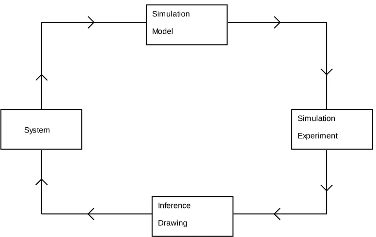
1.4 Principles for Simulation Modeling and Experimentation

(18)

System

Simulation Model

Simulation Experiment

[image:18.612.113.501.68.313.2]

Drawing Inference

Figure 1-2: Simulation for Systems Design and Improvement.

A mathematical-logical form of an existing or proposed system, called a simulation model, is constructed (art). Experiments are conducted with the model that generates numerical results (science). The model and experimental results are interpreted to draw conclusions about the system (art). The conclusions are implemented in the system (science and art).

2. Computer simulation models conform both to system structure and to available

system data (Pritsker, 1989).

Simulation models emphasize the direct representation of the structure and logic of a system as opposed to abstracting the system into a strictly mathematical form. The availability of system descriptions and data influences the choice of simulation model parameters as well as which system objects and which of their attributes can be included in the model. Thus, simulation models are analytically intractable, that is exact values of quantities that measure system performance cannot be derived from the model by mathematical analysis. Instead, such inferencing is accomplished by experimental procedures that result in statistical estimates of values of interest. Simulation experiments must be designed as would any laboratory or field experiment. Proper statistical methods must be used in observing performance measure values and in interpreting experimental results.

3. Simulation supports experimentation with systems at relatively low cost and at

little risk.

Computer simulation models can be implemented and experiments conducted at a fraction of the cost of the P-D-C-A cycle of lean used to improve the future state to reach operational performance objectives. Simulation models are more flexible and adaptable to changing requirements than P-D-C-A. Alternatives can be assessed without the fear that negative consequences will damage day-to-day operations. Thus, a great variety of options can be considered at a small cost and with little risk.

(19)

changed and the results measured, consistent with the lean approach. Alternatively, simulation could be used to assess the impact of the proposed new layout.

4. Simulation models adapt over the course of a project.

As was discussed in the previous section, simulation projects can result in the iterative definition of models and experimentation with models. Simulation languages and software environments are constructed to help models evolve as project requirements change and become more clearly defined over time.

5. A simulation model should always have a well-defined purpose.

A simulation model should be built to address a clearly specified set of system design and operation issues. These issues help distinguish the significant system objects and relationships to include in the model from those that are secondary and thus may be eliminated or approximated. This approach places bounds on what can be learned from the model. Care should be taken not to use the model to extrapolate beyond the bounds.

6. "Garbage in - garbage out" applies to models and their input parameter values

(Sargent, 2009).

A model must accurately represent a system and data used to estimate model input parameter values must by correctly collected and statistically analyzed. This is illustrated in Figure 1-3.

Figure 1-3: Model Validation and Verification.

System

---

Model-Related

Data

Model:

Computer

Implementation

Model:

Specification

(Conceptual

Model)

Verification

(20)

instead of better. This makes simulation and system designers who use it useless in the eyes of management.

7. Variation matters.

A story is told of a young university professor who was teaching an industrial short course on simulation. He gave a lengthy and detailed explanation of a sophisticated technique for estimating the confidence interval of the mean. At the next break, a veteran engineer took him aside and said "I appreciate your explanation, but when I design a system I pretty much know what the mean is. It is the variation and extremes in system behavior that kill me."

Variation has to do with the reality that no system does the same activity in exactly the same way or in the same amount of time always. Of course, estimating the mean system behavior is not unimportant. On the other hand, if every aspect of every system operation always worked exactly on the average, system design and improvement would be much easier tasks. One of the deficiencies of lean is that such an assumption is often implicitly made.

Variation may be represented by the second central moment of a statistical distribution, the variance. For example, the times between arrivals to a fast food restaurant during the lunch hour could be exponentially distributed with mean 10 seconds and, therefore, variance 100 seconds. Variation may also arise from decision rules that change processing procedures based on what a system is currently doing or because of the characteristics of the unit being processed. For instance, the processing time on a machine could be 2 minutes for parts of type A and 3 minutes for parts of type B.

There are two kinds of variation in a system: special effect and common cause. Special effect variation arises when something out of the ordinary happens, such as a machine breaks down or the raw material inventory becomes exhausted because of an unreliable supplier. Simulation models can show the step by step details of how a system responds to a particular special effect. This helps managers respond to such occurrences effectively.

Common cause variation is inherent to a normally operating system. The time taken to perform operations, especially manual ones, is not always the same. Inputs may not be constantly available or arrive at equally spaced intervals in time. They may not all be identical and may require different processing based on particular characteristics. Scheduled maintenance, machine set up tasks, and worker breaks may all contribute. Often, one objective of a simulation study is to find and assess ways of reducing this variation.

Common cause variation is further classified in three ways. Outer noise variation is due to external sources and factors beyond the control of the system. A typical example is variation in the time between customer orders for the product produced by the system. Variational noise is indigenous to the system such as the variation in the operation time for one process step. Inner noise variation results from the physical deterioration of system resources. Thus, maintenance and repair of equipment may be included in a model.

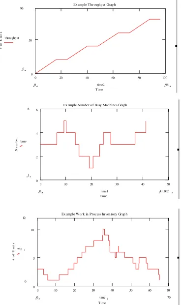
8. Looking at all the simulated values of performance measures helps.

(21)

10

Ex ample Work in Process In ven to ry Grap h

U

n

it

s

12

wip _i

0 20 40 60 80 100

0 50

Ex ample T hroughp ut Grap h

Time

#

o

f

U

n

it

s

96

0 throughput

96

0 time2

0 10 20 30 40 50

0 2 4 6

Ex ample Number o f Busy Machines Graph

Time

N

u

m

b

e

r

6

1 busy

41.062

[image:21.612.71.439.47.667.2]

(22)

The first shows how a special effect, machine failure, results in a build up of partially completed work. After the machine is repaired, the build up declines. The second shows the pattern of the number of busy machines at one system operation over time. The high variability suggests a high level of common cause variation and that work load leveling strategies could be employed to reduce the number of machines assigned to the particular task. The third graph shows the total system output, called throughput, over time. Note that there is no increase in output during shutdown periods, but otherwise the throughput rate appears to be constant.

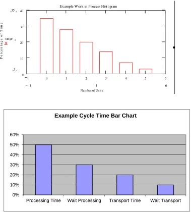
[image:22.612.93.472.220.640.2]

Figure 1-5 shows a sample histogram and a sample bar chart. The histogram shows the sample distribution of the number of discrete parts in a system that appears to be acceptably low most of the time. The bar chart shows how these parts spend their time in the system. Note that one-half of the time was spent in actual processing which is good for most manufacturing systems.

Figure 1-5: Example Histogram and Bar Charts for Performance Measure Observations

1 0 1 2 3 4 5 6

0 10 20 30 40

Ex ample Work in Process Hist ogram

Number of Units

P

e

rc

e

n

ta

g

e

o

f

T

im

e

35

3 range _l

6 1

 l

0% 10% 20% 30% 40% 50% 60%

Processing Time Wait Processing Transport Time Wait Transport

(23)

9. Simulation experimental results conform to unique system requirements for information.

Using simulation, the analyst is free to define and compute any performance measure of interest, including those unique to a particular system. Transient or time varying behavior can be observed by examining individual observations of these quantities. Thus, simulation is uniquely able to generate information that leads to a thorough understanding of system design and operation.

Though unique performance measures can be defined for each system, experience has shown that some categories of performance measures are commonly used:

1. System outputs per time interval (throughput) or the time required to produce a certain amount of output (makespan).

2. Waiting for system resources, both the number waiting and the waiting time.

3. The amount of time, lead time, required to convert individual system inputs to system outputs.

4. The utilization of system resources.

5. Service level, the ability of the system to meet customer requirements.

10. What goes into a model must come out or be consumed.

Every unit entering a simulation model for processing should be accounted for either as exiting the model or assembled with other units or destroyed. Accounting for every unit aids in verification.

11. Results for analytic models should be employed.

Analytic models can be used to enhance simulation modeling and experimentation. Result of analytic models can be used to set lower and upper bounds on system operating parameters such as inventory levels. Simulation experiments can be used to refine these estimates. Analytic models and simulation models can compute the same quantities, supporting validation efforts.

12. Simulation rests on the engineering heritage of problem solving.

Simulation procedures are founded on the engineering viewpoint that solving the problem is of utmost importance. Simulation was born of the necessity to extract information from models where analytic methods could not. Simulation modeling, experimentation, and software environments have evolved since the 1950’s to meet expanding requirements for understanding complex systems.

(24)

1.5 Approach

The fundamental premise of this book is that learning the problems that simulation solves, as well as well as the modeling and experimental methods needed to solve these problems, is fundamental to understanding and using this technique.

Simulation models are built both from knowledge of basic simulation methods and by analogy to existing models. Similarly, computer-based experiments are constructed using basic experiment design techniques and by analogy to previous experiments. This premise is the foundation of this book. First, simulation methods for model building, simulation experimentation, modeling time delays and other random quantities as well as the implementation of simulation experiments on a computer are presented in the remaining chapters in this part of the book.

While each simulation model of each system can be unique, experience has shown that models have much in common. These common elements and their incorporation into models are discussed in chapter 2. These elementary models, as well as extensions, embellishments, and variations of them, are used in building the models employed in the application studies.

Starting in the next part of the book, the simulation project process discussed in section 1.4 is used in application studies involving a wide range of systems. Basic simulation modeling, experimentation, and system design principles presented in part 1 are illustrated in the application study. Additional simulation modeling and experimental methods applicable to particular types of problems are introduced and illustrated. Readers are asked to solve application problems based on the application studies and related simulation principles.

1.6 Summary

Simulation is a widely applicable modeling and analysis method that assists in understanding the design and operations of diverse kinds of systems. A simulation process directs the step by step activities that comprise a simulation project. Basic methods, principles, and experience guide the development and application of simulation models and experiments.

Questions for Discussion

1. List ways of validating a simulation model.

2. Why might building a model graphically be helpful?

3. List the types of variation and tell why dealing with each is important in system design.

4. Differentiate "art" and "science" with respect to simulation.

5. What is the engineering heritage influence on the use of models?

6. Why does variation matter?

7. Why is the simulation project process iterative?

8. How does the simulation project process foster interaction between system experts and simulation modelers?

9. Why must simulation experiments be designed?

10. Why does a simulation project require both a model and an experiment?

(25)

12. List three ways in which the credibility of a simulation model could be established with managers and system experts.

13. Distinguish between verification and validation.

14. Make two lists, one of the simulation project process activities that managers and system experts participate in and one of those that they don’t.

Active Learning Exercises.

1. Create a paper clip assembly line. A worker at the first station assembles two small paper clips. A worker at the second station adds one larger paper clip. One student feeds the first station with two paper clips at random intervals. Another student observes the line to note the utilization of the stations, the number of assemblies in the inter-station buffer, and the number of completed assemblies. Run the assembly line for 2 minutes. Discuss how this exercise is like a simulation model and experiment.

2. Have the students act out the operation of the drive through window of a fast food restaurant in the following steps.

a. Enter line of cars b. Place order

c. Move to pay window d. Pay for order

e. Move to pick-up window f. Wait for order to be delivered g. Depart

(26)

Chapter 2

Simulation Model Building

2.1 Introduction

How simulation models are constructed is the subject of this chapter. A simulation model consists of a description of a system and how it operates. The model is expressed in the form of mathematical and logical relationships among the system components. Model building is the act and art of representing a system with a model (principle 1) to address a well-defined purpose (principle 5).

Since simulation models conform to system structure and available data (principle 2), model building involves some significant judgment and art. Thus, learning to build simulation models includes learning typical ways system components are represented in models as well as how to adapt and embellish these modeling strategies to each system.

Model building is greatly aided by using a simulation language that provides a set of standard, pre-defined modeling constructs. These modeling constructs are combined to construct models. A simulation software environment provides the user interface and functionality for model construction.

This chapter presents common system components: arrivals, operations, routing, batching, and inventories, as well as describing typical models of each component. These models of components can be combined, extended and embellished to form models of entire systems. Elementary modeling constructs commonly found in simulation languages are presented. The use of these constructs in modeling the common system components is illustrated.

2.2 Elementary Modeling Constructs

This section presents the model building perspective taken in this text. Basic modeling constructs are presented.

The operation of many systems can be effectively described by the sequence of steps taken to transform the inputs to the outputs as shown in a value stream map. This will be our perspective for model building. A sequence of steps specified in a model is called a process. A model consists of one or more such processes.

The modeling construct used to represent the part, customer, information, etc. that is transformed from an input to an output by the sequence of processing steps is an entity. Each individual entity is tracked as it moves through the processing steps. Processing can be unique for each entity with respect to such things as processing times and route through the steps. Thus, it is essential to be able to differentiate among the entities. This is accomplished by associating a unique set of quantities, called attributes, with each entity. Typical attributes include time of arrival to the system and type of part, customer, or other information.

Note that a value stream map shows in general how parts flow through a system. This might be viewed as a “macro” or big picture view of how a system operates. One characteristic of beyond lean is the use of models that give a more detailed or “micro” representation of a system. This helps in gaining of understanding of how a future state will actually operate and aids in ensuring a successful transformation.

(27)

A resource has at least two states, unique circumstances in which it can be. One of these is busy, for example in use operating on an entity. Another is idle, available for use. Typical model logic requires an entity to wait for the resource (or resources) required for a particular processing step to be in the idle state before beginning that step. When the processing step is begun, the resources enter the busy state. As many resource states as necessary may be defined and used in a model. Other common resource states are broken and under repair, off shift and unavailable, and in setup for a new part type.

Consider a workstation consisting of two machines. A basic modeling issue is: Should each machine be modeled using a distinct resource? Often, it does not matter which of the two machines is used to process an entity and operating information such as utilization is not required for each machine. In such a case, it is simpler to use a single resource to model the two machines. However, an additional concept: number of units, is necessary to model two (or mores) machines with one resource. There is one unit of the resource for each machine, two in this example.

State variables, and their values, describe the conditions in a system at any particular time.

State variables must be included in a simulation model and typically include the number of units of each resource in each possible resource state as well as the number of entities waiting for idle units of each resource, the number of entities that have completed processing, and inventory levels.

Time is a significant part of simulation models of systems. For example, when in simulated time

each process step begins and ends for each entity processed by that step must be determined. Sequencing what happens to each entity correctly in time, and thus correctly with respect to what happens to all other entities, must be accomplished.

In summary, modeling the behavior of a system over time requires specifying how the entities use the resources to perform the steps of a process as well as how the values of the entity

attributes and of the state variables, including the state of the units of each resource, change.

2.3 Models of System Components

Typical system components include arrivals, operations, routing, batching, and inventories. Models of these components are presented in this section. The models may be used directly, modified, extended, and combined to support the construction of new models of entire systems.

2.3.1 Arrivals

(28)

Suppose that time between arrivals varies. This implies that the time between arrivals is described by some probability distribution whose mean is the average time between arrivals. The variance of the distribution characterizes how much the individual times between arrivals differ from each other. For example, suppose the time between arrivals is exponentially distributed with mean 10 seconds, implying a variance of 10*10 = 100 seconds2. The first arrival is at time 0. The second arrival could be at time 25 seconds, the third at time 31 seconds, the fourth at time 47 seconds, and so forth. Thus, the arrival process is a source of outer noise.

An example specification in pseudo-English follows.

Define Arrivals: // mean must equal takt time Time of first arrival: 0

Time between arrivals: Exponentially distributed with a mean of 10 seconds Exponential (6) seconds

Number of arrivals: Infinite

2.3.2 Operations

The next issue encountered when modeling the single machine workstation in Figure 2-1 is specifying how the entities are processed by the workstation. Each entity must wait in the buffer (queue) preceding the machine. When available, the machine processes the entity. Then the entity departs the workstation.

A workstation resource is defined with the name WS to have 1 unit with states BUSY and IDLE using the notation WS/1: States(BUSY, IDLE). It is assumed that all units of a resource are initially IDLE. The operation of the machine is modeled as follows. Each entity waits for the single unit of the WS (workstation) resource to be available to operate on it that is the WS resource to be in the IDLE state. At the time processing begins WS becomes BUSY. After the operation time, the entity no longer needs WS, which becomes IDLE and available to operate on the next entity.

(29)

Define Resources:

WS/1 with states (Busy, Idle)

Process Single Workstation Begin

Wait until WS/1 is Idle in Queue QWS // part waits for its turn on the machine

Make WS/1 Busy // part starts turn on machine; machine is busy Wait for OperationTime // part is processed

Make WS/1 Idle // part is finished; machine is idle End

Note the pattern of resource state changes. For every process step that makes a resource enter the busy state, there must be a corresponding step that makes the resource enter the idle state. However, there may be many process steps between these two corresponding steps. Thus, many operations may be performed in sequence on an entity using the same resource.

Note also the two types of wait statements that delay entity movement through a process. Wait for means wait for a specified amount of simulation time to pass. Wait unit means wait until a state variable value meets a specified logical condition. This is a very powerful construct that also is consistent with ideas in event-based programming.

Consider another variation on the single machine workstation operation that illustrates the use of conditional logic in a simulation model. The machine requires a setup operation of 1.5 minutes duration whenever the Type of an entity differs from the Type of the preceding entity processed by the machine. For example, the machine may require one set of operational parameter settings when operating on one type of part and a second set when operating on a second type of part. The model of this situation is as follows.

Define Resources:

WS/1 with states (Busy, Idle, Setup)

Define State Variables: LastType

Define Entity Attributes: Type

Process Single Workstation with Setup Begin

Wait until WS/1 is Idle in Queue QWS // part waits for its turn on the machine

(30)

types. Such logic is common in simulation models and makes most of them analytically intractable. A new state, SETUP, is defined for WS. This resource enters the SETUP state when the setup operation begins and returns to the BUSY state when the setup operation ends.

Often a workstation is subject to interruptions. In general, there are two types of interruptions: scheduled and unscheduled. Scheduled interruptions occur at predefined points in time. Scheduled maintenance, work breaks during a shift, and shift changes are examples of scheduled interruptions. The duration of a scheduled interruption is typically a constant amount of time. Unscheduled interruptions occur randomly. Breakdowns of equipment can be viewed as unscheduled interruptions. An unscheduled interruption typically has a random duration.

A generic model of interruptions is shown in Figure 2-2. An interruption occurs after a certain amount of operating time that is either constant or random. The duration of the interrupt is either constant or random. After the end of the interruption, this cycle repeats.

Note that the transition to the INTERRUPTED state is modeled as occurring from the IDLE state. Suppose the resource is in the BUSY state when the interruption occurs. Typically, a simulation engine will assume that the resource finishes a processing step before entering the INTERRUPTED state. However, the end time of the interruption will be the same that is the amount of time in the INTERRUPTED state will be reduced by the time spent after the interruption occurs in the BUSY state. This approximation normally has little or no effect on the simulation results. In many systems, interruptions are often only detected or acted upon at the end of an operation. Using this approximation avoids having to include logic in the model as to what to do with the entity being processed when the interruption occurs. On the other hand, such logic could be included in the model if required.

This breakdown-repair process may be expressed in statements as follows:

Define Resource:

WS/1: States(Busy, Idle, Unavailable)

Process Breakdown—Repair Begin

Do While 1=1 // Do forever

Wait for TimeBetweenBreakdowns Wait until WS/1 is Idle

Make WS/1 Unavailable Wait for RepairTime Make WS/1 Idle End Do

End

Consider an extension of the model of the single machine workstation with breakdowns (random interruptions) added. This model combines the process model for the single workstation with the process model for breakdown and repair. The WS resource now has three states: BUSY operating on an entity, IDLE waiting for an entity, and UNAVAILABLE during a breakdown. This illustrates how a model can consist of more than one process.

(31)

(32)

2.3.3 Routing Entities

In many systems, decisions must be made about the routing of entities from operation to operation. This section discusses typical ways systems make such routing decisions as well as techniques for modeling them. A distinct process for making the routing decision can be included in the model.

Consider a system that processes multiple item types using several workstations. Each workstation performs a unique function. Each job type is operated on by a unique sequence of workstations called a route. In a manufacturing environment, this style of organization is referred to as a job shop. It could also represent the movement of customers through a cafeteria where different foods: hot meals, sandwiches, salads, desserts, and drinks are served at different stations. Customers are free to visit the stations in any desired sequence.

Each entity in the model of a job shop organization could have the following attributes:

ArrivalTime: Time of arrival

Type: The type of job, which implies the route.

Location: The current location on the route relative to the beginning of the route.

In addition, the model needs to store the route for each type of job.

Suppose there are four workstations and three job types in a system. Figure 2-3 shows a possible set of routings in matrix form.

Job Type First Operation Second Operation Third Operation Fourth Operation

1 Workstation 1 Workstation 2 Workstation 3 Workstation 4

2 Workstation 3 Workstation 4 None None

3 Workstation 4 Workstation 2 Workstation 3 None

Figure 2-3: Example Routing Matrix for A Manufacturing Facility.

A routing process is included in the simulation model to direct the entity to the workstation performing the next processing step. The routing process requires zero simulation time.

Define State Variable: Route(3, 4)

Define Attribute: Location

Define Attribute: Type

Process Routing Begin

Location += 1

If Route(Type, Location) != None Then Begin

Send to Process Route(Type, Location) End

Else Begin

Send to Process Depart End

(33)

The value of the Location attribute is incremented by one. The next workstation to process the entity is the one at matrix location (Type, Location). If this matrix location has a value of None, then processing of the entity is complete. Note again that the ability to compose a model of multiple processes is important.

Alternatively, routes may be selected dynamically based on current conditions in a system as captured in the values of the state variables. Such decision making may be included in a simulation model. This is another unique and very powerful capability of simulation modeling.

Consider a highly automated system in which parts wait in a central storage area for processing at any workstation. A robot moves the parts between the central storage area and the workstations. Alternatively if the following workstation is IDLE when an operation is completed, the robot moves the part directly to the next workstation instead of the storage area. The routing process for this situation follows, where WSNext is the resource modeling the following workstation.

_____________________________________________________________________________ Define Resource:

WSNext/1: States(Busy, Idle) Define State Variable:

CentralStorage

Process Conditional Routing Begin

If WSNext/1 is Idle Then Begin

Send to Process ForWSnext End

Else Begin

CentralStorage += 1 End

End

2.3.4 Batching

Many systems use a strategy of grouping items together and then processing all the items in the group jointly. This strategy is called batching. Batching may occur preceding a machine on the factory floor. Parts of the same type are grouped and processed together in order to avoid frequent setup operations. Other examples include:

 Bags of product may be stacked on a pallet until its capacity is reached. Then a forklift could be used to load the pallet on a truck for shipment.

(34)

Returning to the single server workstation example of Figure 2-2, suppose that completed parts are transported in groups of 20 from the output buffer to input buffer of a second workstation some distance away. At the second workstation, items are processed individually. In the simulation model of this situation, the first 19 entities, each modeling an item to be transported, must wait until the twentieth entity arrives. Then the 20 entities are moved together as a group. Each group is referred to as a batch. Upon arrival at the second workstation, each entity individually enters the workstation buffer. The batching and un-batching extension to the single server workstation model is as follows.

Define Resource: WS/1: States(Busy, Idle) Define List: OutputBuffer

Process Single Workstation with Output Buffer Begin

Wait until WS/1 is Idle Make WS/1 Busy Wait for Operation Time Make WS/1 Idle

If Length (OutputBuffer) < 19 then Begin

Add to List(OutputBuffer) End

Else Begin

Wait for Transportation Time

Send All Entities on List(OutputBuffer) to Process WS2 End

End

Consider the case where each of the types of items processed by the workstation must be transported separately. In this situation, batching, transportation, and un-batching can be done as above except one batch is formed for each type of item.

2.3.5 Inventories

In many systems, items are produced and stored for subsequent use. A collection of such stored items is called an inventory, for example televisions waiting in a store for purchase or hamburgers under the hot lamp at a fast food restaurant. Customers desiring a particular item must wait until one is inventory.

Inventory processes have to do with adding items to an inventory and removing items from an inventory. The number of items in an inventory can be modeled using a state variable, for example INV_LEVEL. Placing an item in inventory is modeled by adding one to the state variable: INV_LEVEL += 1. Modeling the removal of an item from an inventory requires two steps:

1. Wait for an item to be in the inventory: WAIT UNTIL INV_LEVEL > 0 2. Subtract one from the number of items in the inventory: INV_LEVEL -= 1

2.4 Summary

(35)

Problems

1. Discuss why it is important to be able to employ previously developed models of system components in addition to the more basic modeling constructs provided by a simulation language in model building.

2. Discuss the importance of allowing multiple, parallel processes in a model.

(For each of the modeling problems that follow, use the pseudo-English code that has been presented in this chapter.)

3. Develop a model of a single workstation whose processing time is a constant 8 minutes. The station processes two part types, each with an exponentially distributed interarrival time with mean 20 minutes.

4. Embellish the model developed in 3 to include breakdowns. The time between breakdowns in exponentially distributed with mean 2 days. Repair time is uniformly distributed between 1 and 3 hours.

5. Build a model of a two-station assembly line serving three types of parts. The sequence of part types is random. The part types are distributed as follows: part type 1, 30%; part type 2; 50%, and part 3, 20%. Inter-arrival time is a constant 5 minutes. The first station requires a setup task of 1.5 minutes duration whenever the current part type is different from the preceding one. The operation times are the same regardless of part type: station 1, 3 minutes and station 2, 4 minutes.

6. Embellish the model in problem 5 for the case where there are two stations that perform the second operation. The part goes to the station with the fewer number of waiting parts.

7. Embellish the model in problem 5 for the case where a robot loads and unloads the second station. Loading and unloading each take 15 seconds.

8. Combine problems 5, 6, and 7 in one model.

(36)

12. Develop a process model of the following situation. Two types of parts are processed by a station. A setup time of one minute is required if the next part processed is of a different type that the preceding part. Processing time at the station is the same for both part types: 10 minutes. Type 1 parts arrive according to an exponential distribution with mean 20 minutes. Type 2 parts arrive at the constant rate of 2 per hour.

13. Develop a process model of the following situation. A train car is washed and dried in a rail yard between each use. The same equipment provides for washing and drying one car at a time. Washing takes 30 minutes and drying one hour. Cars arrive at the constant rate of one each hour and three-quarters.

14. Develop a model of a service station with 10 self-service pumps. Each pump dispenses each of three grades of gasoline. Customer service at the pump time is uniformly distributed between 30 seconds and two minutes. One-third of the customers pay at the pump using a credit card. The remainder must pay a single inside cashier which takes an additional 1 minute to 2 minutes, uniformly distributed. The time between arrivals of cars is exponentially distributed with mean 1 minute.

15. Mike’s Market has three check out lanes each with its own waiting line. One check out lane is for customers with 10 items or fewer. The check out time is 10 seconds plus 2 seconds per item. The number of items purchased is triangularly distributed with minimum 1, mode 10, and maximum 100. The time between arrivals to the check-out lanes is exponentially distributed with mean 1 minute.

16. Develop a more detailed model of Bob’s Burger Barn (discussed in problem 9). Add an