197 CANDIDATES AND 104 VALIDATED PLANETS IN
K2ʼ
s FIRST FIVE FIELDS
Ian J. M. Crossfield1,28,30, David R. Ciardi2, Erik A. Petigura3,31, Evan Sinukoff4,32, Joshua E. Schlieder2,5,33, Andrew W. Howard4, Charles A. Beichman2, Howard Isaacson6, Courtney D. Dressing3,30, Jessie L. Christiansen2,
Benjamin J. Fulton4,34, Sébastien Lépine7, Lauren Weiss6, Lea Hirsch6, John Livingston8, Christoph Baranec9, Nicholas M. Law10, Reed Riddle11, Carl Ziegler10, Steve B. Howell5, Elliott Horch12, Mark Everett13, Johanna Teske14, Arturo O. Martinez7,15, Christian Obermeier16, Björn Benneke3, Nic Scott17, Niall Deacon18, Kimberly M. Aller4, Brad M. S. Hansen19, Luigi Mancini16, Simona Ciceri16,20, Rafael Brahm21,22, Andrés Jordán21,22,
Heather A. Knutson3, Thomas Henning16, Michaël Bonnefoy23,24, Michael C. Liu4, Justin R. Crepp25, Joshua Lothringer1, Phil Hinz26, Vanessa Bailey26,27, Andrew Skemer26,28, and Denis Defrere23,24,29
1
Lunar & Planetary Laboratory, University of Arizona, 1629 E. University Boulevard., Tucson, AZ, USA 2
NASA Exoplanet Science Institute, California Institute of Technology, Pasadena, CA, USA 3
Geological and Planetary Sciences, California Institute of Technology, Pasadena, CA, USA 4
Institute for Astronomy, University of Hawai‘i at Mānoa, Honolulu, HI, USA 5
NASA Ames Research Center, Moffett Field, CA, USA 6
Astronomy Department, University of California, Berkeley, CA, USA 7
Department of Physics and Astronomy, Georgia State University, GA, USA 8
Department of Astronomy, The University of Tokyo, 7-3-1 Bunkyo-ku, Tokyo 113-0033, Japan 9
Institute for Astronomy, University of Hawai‘i at Mānoa, Hilo, HI, USA 10
Department of Physics and Astronomy, University of North Carolina at Chapel Hill, Chapel Hill, NC, USA 11
Division of Physics, Mathematics, and Astronomy, California Institute of Technology, Pasadena, CA, USA 12
Department of Physics, Southern Connecticut State University, New Haven, CT, USA 13
National Optical Astronomy Observatory, Tucson, AZ, USA 14
Carnegie Department of Terrestrial Magnetism, Washington, DC, USA 15
Department of Astronomy, San Diego State University, San Diego, CA, USA 16
Max Planck Institut für Astronomie, Heidelberg, Germany 17
Sydney Institute of Astronomy, The University of Sydney, Redfern, Australia 18
Centre for Astrophysics Research, University of Hertfordshire, UK 19
Department of Physics & Astronomy and Institute of Geophysics & Planetary Physics, University of California Los Angeles, Los Angeles, CA, USA 20
Department of Astronomy, Stockholm University, SE-106 91 Stockholm, Sweden 21
Millennium Institute of Astrophysics, Av. Vicuña Mackenna 4860, 7820436 Macul, Santiago, Chile 22
Instituto de Astrofísica, Facultad de Física, Pontificia Universidad Católica de Chile, Av. Vicuña Mackenna 4860, 7820436 Macul, Santiago, Chile 23
Univ. Grenoble Alpes, IPAG, F-38000, Grenoble, France 24
CNRS, IPAG, F-38000, Grenoble, France 25
Department of Physics, University of Notre Dame, 225 Nieuwland Science Hall, Notre Dame, IN, USA 26
Steward Observatory, The University of Arizona, Tucson, AZ, USA 27
Kavli Institute for Particle Astrophysics and Cosmology, Stanford University, Stanford, CA, USA 28
Department of Astronomy, University of California, Santa Cruz, Santa Cruz, CA, USA 29
Departement d’Astrophysique, Geophysique et Oceanographie, Universite de Liege, B-4000 Sart Tilman, Belgium Received 2016 April 1; revised 2016 June 20; accepted 2016 June 20; published 2016 September 2
ABSTRACT
We present 197 planet candidates discovered using data from thefirst year of the NASAK2mission(Campaigns 0–4), along with the results of an intensive program of photometric analyses, stellar spectroscopy, high-resolution imaging, and statistical validation. We distill these candidates into sets of 104 validated planets(57 in multi-planet systems),30false positives, and 63 remaining candidates. Our validated systems span a range of properties, with median values ofRP=2.3RÅ,P=8.6days,Teff=5300K, and Kp=12.7mag. Stellar spectroscopy provides precise stellar and planetary parameters for most of these systems. We show that K2has increased by 30% the number of small planets known to orbit moderately bright stars(1–4R⊕,Kp=9–13mag). Of particular interest are76planets smaller than 2R⊕,15orbiting stars brighter thanKp=11.5mag, 5 receiving Earth-like irradiation levels, and several multi-planet systems—including 4 planets orbiting the M dwarf K2–72 near mean-motion resonances. By quantifying the likelihood that each candidate is a planet we demonstrate that our candidate sample has an overall false positive rate of 15%–30%, with rates substantially lower for small candidates (<2RÅ)and larger for candidates with radii >8RÅ and/or with P<3 days. Extrapolation of the current planetary yield suggests thatK2will discover between 500 and 1000 planets in its planned four-year mission, assuming sufficient follow-up resources are available. Efficient observing and analysis, together with an organized and coherent follow-up strategy, are essential for maximizing the efficacy of planet-validation efforts forK2,TESS, and future large-scale surveys.
© 2016. The American Astronomical Society. All rights reserved.
30
NASA Sagan Fellow. 31
Hubble Fellow.
32NSERC Postgraduate Research Fellow. 33
NASA Postdoctoral Program Fellow. 34
Key words:catalogs–planets and satellites: fundamental parameters–planets and satellites: general–techniques: high angular resolution– techniques: photometric– techniques: spectroscopic
Supporting material:machine-readable tables
1. INTRODUCTION
Planets that transit their host stars offer unique opportunities to characterize planetary masses, radii, and densities; atmo-spheric composition, circulation, and chemistry; dynamical interactions in multi-planet systems; and orbital alignments and evolution, to name just a few aspects of interest. Transiting planets are also the most common type of exoplanet known, thanks in large part to NASA’s Kepler spacecraft. Data from
Kepler’s initial four-year survey revealed over 4000 candidate exoplanets and many confirmed and validated planets35 (e.g., Coughlin et al. 2016; Morton et al. 2016). A majority of all exoplanets known today were discovered byKepler. After the spacecraft’s loss of a second reaction wheel in 2014, the mission was renamedK2and embarked on a new survey of the ecliptic plane, divided into campaigns of roughly 80 days each (Howell et al. 2014). In terms of survey area, temporal coverage, and data release strategy, K2 provides a natural transition fromKeplerto theTESSmission(Ricker et al.2014).
Kepler observed 1/400th of the sky for four years (initially with a default proprietary period), while TESS will observe nearly the entire sky for 27 days,36 with no default proprietary period.
In its brief history K2 has already made many new discoveries. The mission’s data have helped to reveal oscillations in variable stars(Angus et al.2016)and discovered eclipsing binaries(LaCourse et al.2015; Armstrong et al.2016; David et al. 2016a), supernovae (Zenteno et al. 2015), large numbers of planet candidates (Foreman-Mackey et al. 2015; Adams et al. 2016; Vanderburg et al. 2016), and a growing sample of validated and/or confirmed planets (e.g., Vander-burg & Johnson 2014; Crossfield et al. 2015; Huang et al.
2015; Montet et al. 2015; Sanchis-Ojeda et al.2015; Sinukoff et al. 2016). Here, we report our identification and follow-up observations of 197 candidate planets usingK2data. Using all available observations and a robust statistical framework, we validate 104 of these as true, bona fide planets, and for the remaining systems we discriminate between obvious false positives and a remaining subset of plausible candidates suitable for further follow-up.
In Section 2 we review our target sample, photometry and transit search, and initial target vetting. Section3describes our supporting ground-based observations(stellar spectroscopy and high-resolution imaging; HRI), while Section 4 describes our derivation of stellar parameters. These are followed by our intensive transit light curve analysis in Section 5, the assessment of FPPs for our candidates in Section 6, and a discussion of the results, interesting trends, and noteworthy individual systems in Section 7. Finally, we conclude and summarize in Section8.
2. K2 TARGETS AND PHOTOMETRY
2.1. Target Selection
In the analysis that follows we use data from allK2targets (not just those in our own General Observer proposals37). Huber et al.(2016)present the full distribution of stellar types observed byK2. For completeness we describe here our target selection strategy, which has successfully proposed for thousands of FGK and M dwarfs through two parallel efforts. We select our FGK stellar sample from the all-sky TESS
Dwarf Catalog(TDC; Stassun et al.2014). The TDC consists of 3 million F5–M5 candidate stars selected from 2MASS and cross-matched with the NOMAD, Tycho-2, Hipparcos, APASS, and UCAC4 catalogs to obtain photometric colors, proper motions, and parallaxes. We remove giant stars based on reduced proper motion versus J−H color (see Collier Cameron et al.2007), and generate a magnitude-limited dwarf star sample from the merged TDC/EPIC by requiring
Kp<14mag for these FGK stars. We impose an anti-crowding criterion and remove all targets with a second star in EPIC (complete down toKp∼19 mag; Huber et al.2016)within 4 arcsec(approximately theKeplerpixel size). This last criterion removes <1% of the FGK stars in our proposed samples, improves catalog reliability by reducing false positives, and simplifies subsequent vetting and Doppler follow-up.
We draw our late-type (K and M dwarf) stellar sample primarily from the SUPERBLINK proper motion database(SB, Lépine & Shara 2005) and the PanSTARRS-1 survey (PS1, Kaiser2002). We use a combination of reduced proper motion, optical/NIR color cuts, and/or SED fitting to capture the majority of M dwarfs (>85%) within 100 pc with little contamination from distant giants. In some K2campaigns we supplement our initial database using SDSS, PS1, and/or other photometry to identify additional targets with smaller proper motions(following Aller et al.2013). We estimate approximate spectral types (SpTs) using tabulated photometric relations (Kraus & Hillenbrand 2007; Pecaut & Mamajek 2013; Rodriguez et al. 2013) and convert SpTs into stellar radii (R*) based on interferometric studies (Boyajian et al. 2012). Our exact selection criteria for K and M dwarfs have evolved with time, but we typically prioritize this low-temperature stellar sample by requiring a signal-to-noise ratio (S/N)8 for a single transit of an Earth-sized planet, assuming the demonstrated photometric precision ofK2. We additionally set a magnitude limit of Kp<16.5 mag on this late-type dwarf sample to allow feasible spectroscopic characterization.
2.2. Time-series Photometry
Our team’s photometric pipeline(described by, e.g.,
Cross-field et al. 2015; Petigura et al. 2015builds on the approach originally outlined by Vanderburg & Johnson (2014). We extract time-series photometry from the target pixel files provided by the project using circular, stationary, soft-edged apertures. During K2 operations, solar radiation pressure 35
We distinguish “confirmed” systems (with measured masses) from
“validated” systems (whose planetary nature has been statistically demon-strated, e.g., with false positive probability(FPP)<1%).
36
Smaller fractions of the sky will be observed for up to 351 days.
torques the spacecraft, causing it to roll around the boresight. This motion causes a typical target star to drift across the CCD by∼1 pixel every∼6 hr. This motion of stars across the CCD, when combined with inter- and intra-pixel sensitivity variations and aperture losses, results in significant changes in our aperture photometry.
We remove these stellar brightness variations that correlate with spacecraft orientation by first solving for the roll angle between each frame and an arbitrary reference frame using roughly 100 stars of Kp∼12 mag on an arbitrary output channel. Then, we model the time- and roll-dependent brightness variations using a Gaussian process with a squared-exponential kernel. We apply apertures with radii ranging from 1 to 7 pixels and select the aperture that minimizes the residual noise in the corrected light curve (computed on three-hour timescales). This minimization balances two competing effects: larger apertures yield smaller systematic errors (because aperture losses are smaller), while smaller apertures incur less background noise. All of our processed light curves are available for download at the NExScI ExoFOP website.38
2.3. Identifying Transit-like Signals
We search our calibrated photometry for planetary transits using the TERRA algorithm (Petigura et al. 2013a). After running TERRA, we flag stars with putative transits having S/N>12 as threshold-crossing events (TCEs) for visual inspection. Below this level, transit signals surely persist but TCEs become dominated by spurious detections. Residual outliers in our photometry prevent us from identifying large numbers of candidates at lower S/N. In order to reduce the number of spurious detections we require that TCEs have orbital periods P1 days, and that they also show three transits. This last criterion sets an upper bound to the longest period detectable in our survey at half the campaign baseline, or ∼37 days.39Thus many longer-period planets likely remain to be found in these data sets, in a manner analogous to the discovery of HIP-116454b in K2’s initial engineering run (Vanderburg et al. 2016) and additional single-transit candi-dates identified in Campaigns 1–3(Osborn et al.2016).
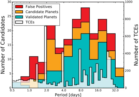
In our analysis, each campaign yields roughly 1000 TCEs. The distribution of their orbital periods, shown in Figure 1, reveals discrete peaks atP=1.5, 2, 4, 8, and 16 days. These sharp peaks likely correspond to the 6 hr periodicity of small-scale maneuvering tweaks to rebalance solar pressure and/or to the 48 hr periodicity ofK2’s reaction wheel momentum dumps (Van Cleve et al. 2016). Both these effects could induce correlated photometric jitter on integer multiples of this timescale. We also see a smoother increase in TCEs toward longer periods(P16 days)that our manual vetting(described below)shows as corresponding to an increasing false positive rate(FPR)for TCEs showing just 3–5 transit-like events.
In each campaign, our manual vetting process begins with these TCEs and results in well-defined lists of astrophysical variables, including robust planet candidates for further follow-up and validation. TERRA produces a set of diagnostics for every TCE with a detection above our S/N limit, which we use to determine whether the event was likely caused by a
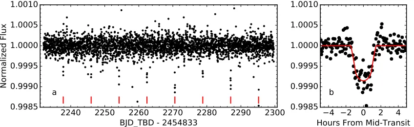
candidate planet, eclipsing binary, periodic variable, or noise. The diagnostics include a summary of basicfit parameters and a suite of diagnostic plots to visualize the nature of the TCE. These plots include the TERRA periodogram, a normalized phase-folded light curve with a best-fit model, the light curve phased to 180°to look for eclipses or misidentified periods, the most probable secondary eclipse identified at any phase, and an autocorrelation function. When vetting, the userflags each TCE as an object of interest or not, where objects of interest can be either candidate planets, eclipsing binaries, or variable stars. We elevate any TCE showing no obvious warning signs to the status of“planet candidate,”i.e., an event that is almost surely astrophysical in nature, possibly a transiting planet, and not obviously a false positive scenario like a background eclipsing binary. We quantify the FPPs of all our candidates in Section6. Figure2shows an example of aTERRA-derived light curve for a typical candidate.
Once we identify a candidate, we re-runTERRAto search for additional planets in that system as described by Sinukoff et al. (2016). In brief, we mask out the photometry associated with transits of the previously identified candidate and runTERRA again to look for additional box-shaped signals. We repeat this process until no candidates are identified with S/N>8 or the number of candidates exceeds five. We typically find <10 multi-candidate systems per campaign, with a maximum of four planets detected per star.
3. SUPPORTING OBSERVATIONS
3.1. High-resolution Spectroscopy: Observations
3.1.1. Keck/HIRES
[image:3.612.322.566.52.223.2]We obtained high-resolution optical spectra of 83 planet candidate hosts using the HIRES echelle spectrometer (Vogt1994)on the 10 m Keck I telescope. These spectra were collected using the standard procedures of the California Planet Search(CPS; Howard et al. 2010). We used the“C2”decker (0. 87 ´14 slit), which is long enough to simultaneously measure the spectra of the target star and the sky background
Figure 1.Distribution of orbital periods of transit-like signals identified in our analysis. The pale, narrow-binned histogram (axis at right) indicates the Threshold-Crossing Events(TCEs)identified byTERRAin our initial transit search (see Section 2). The coarser histograms (axis at left) indicate the cumulative distributions of 104 validated planets(blue-green; FPP<0.01),30
false positive systems(red; FPP>0.99), and 63 candidates of indeterminate status(orange).
38
https://exofop.ipac.caltech.edu 39
with spectral resolution R=55,000. The sky was subtracted from each stellar spectrum. We used the HIRES exposure meter to automatically terminate each exposure once the desired S/N was reached, typically after 1–20 minutes. For stars with
V<13.0mag, exposure levels were set to achieve S/N=45 per pixel at 550 nm. Exposures of fainter stars were terminated at S/N=32 per pixel—enough to derive stellar parameters while keeping exposure times reasonable. For stars that were part of subsequent Doppler campaigns, we measured additional HIRES spectra with higher S/N. These RV measurements will be the subject of a series of forthcoming papers.
3.1.2. Automated Planet Finder(APF)/Levy
We obtained spectra of 27 candidate host stars using the Levy high-resolution optical spectrograph mounted at the APF. Each spectrum covers a continuous wavelength range from 374 to 970 nm. We observed the stars using either the 2″×8″slit for a spectral resolution of R≈80,000, or, to minimize sky contamination, the 1″×3″ slit for a spectral resolution of
R≈100,000. We initially observed all bright targets using the 2″×8″ slit to maximize S/N but soon noticed that sky contamination was a serious problem on nights with a full or gibbous moon. All APF spectra collected after 2015 May 21 were observed using the 1″×3″ decker. In all cases, we collected three consecutive exposures and combined the extracted 1D spectra using a sigma-clipped mean to reject cosmic rays. All targets were observed at just a single epoch. Thefinal S/N of the combined spectra ranges from roughly 25 to 50 per pixel.
3.1.3. MPG 2.2 m/FEROS
We obtained spectra of a small number of candidate stellar hosts using the FEROSfiber-fed echelle spectrograph(Kaufer & Pasquini1998)at the 2.2 m MPG telescope. Each spectrum covers a continuous wavelength range from 350 to 920 nm with an average resolution of R∼48,000. Our FEROS exposure times were chosen according to the brightness of each target and ranged from 10 to 30 minutes. Simultaneously with the science images we acquired spectra of a ThAr lamp for wavelength calibration.
The FEROS data are processed through a dedicated pipeline built from a modular code(CERES, R. Brahm et al. 2016, in preparation)designed to reduce, extract and analyze data from different echelle spectrographs in an automated, homogeneous and robust way. This pipeline is similar to the calibration and optimal extraction approach described by Jordán et al. (2014).
We compute a global wavelength solution from the calibration ThAr image byfitting a Chebyshev polynomial as function of the pixel position and echelle order number. The instrumental velocity drifts during the night are computed using the the extracted spectra of the ThAr lamp acquired during the science observations with the reference fiber. The barycentric correc-tion is performed using the JPLephem package. Radial velocities (RVs) and bisector spans are determined by cross-correlating the continuum-normalized stellar spectrum with a binary mask derived from a G2 dwarf’s spectrum (for more details see, e.g., Baranne et al. 1979; Queloz 1995). We normalize the stellar continuum to minimize the systematic errors that would be induced in the derived velocity by differences in spectral slope caused by different reddening or stellar type.
3.2. High-resolution Spectroscopy: Methods and Results
As part of our false positive analysis(described in Section6), we use our high-resolution Keck/HIRES spectra to search for additional spectral lines in the stellar spectra. This method is sensitive to secondary stars that lie within 0 4 of the primary star(one half of the slit width)and that are as faint as 1% of the apparent brightness of the primary star(Kolbl et al.2015). The approach therefore complements the AO and speckle imaging described in Section3.3(Ciardi et al.2015; Teske et al.2015). The search for secondary lines in the HIRES spectra begins with a match of the primary spectrum to a catalog of nearby, slowly rotating, FGKM stars from the CPS. The best match from the catalog is identified, subtracted from the primary spectrum, and the residuals are then searched(using the same catalog)to identify any fainter second spectrum. This method is insensitive to companion stars with velocity offsets of
10 km s−1, in which cases multiple stellar lines would be blended too closely together. This method is optimized for slowly rotating FGKM stars, so stars earlier than F and those with vsini > 10 km s-1 are more difficult to detect due to
their having fewer and/or broader spectral lines. The technique is less sensitive for stars withTeff3500K due to the small number of such stars in the CPS catalog. The derived constraints for all targets are listed in Table 3, and we use them in our false positive analysis described in Section 6. Figure 3 shows an example of a Keck/HIRES spectrum, together with the secondary line search results and derived stellar parameters(see Section4).
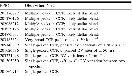
[image:4.612.96.520.52.182.2]We performed a similar analysis for the subset of stars observed by the FEROS spectrograph. Table1lists these stars,
most of which host candidate hot Jupiters. Three show obvious signs of multiple peaks in the stellar cross-correlation, indicating these sources are blends of multiple stars; a fourth shows an extremely high rotational velocity. As described in Section6, wefind FPPs of>50% for all four of these systems, indicating that most are likely false positives and low-priority targets for future follow-up.
By obtaining FEROS spectra at multiple epochs, we detect RV variations from EPIC205148699 in phase with the transit signal and with semi-amplitudeK~28kms−1, indicating that this system is an eclipsing stellar binary. For EPIC201626686, 11 RV measurements over 40 days reveal variations at the level of±50ms−1. Since these variations are not in phase with the orbital period of the detected transits, we do not consider this system to be a false positive. Finally, multiple RV measure-ments also set as an upper limit on the RV variations of K2-24 (EPIC 203771098)of<20 ms−1(consistent with the analysis of Petigura et al. 2016). Our analysis in Section 6 ultimately
finds FPP<0.01for all three of these systems, indicating that these are validated planets.
Single-epoch FEROS observations reveal that both K2-19 (EPIC 201505350)and EPIC 201862715 are single-lined dwarf stars, consistent with our validation of the former(the latter has a close stellar companion that prevents us from validating the system; see Section6). A second observation of K2-19 taken three days later shows an RV variation of∼20ms−1, roughly consistent with the RV signal reported by Barros et al.(2015).
3.3. High-resolution Imaging
3.3.1. Observations
[image:5.612.97.513.53.295.2]We obtained HRI for 164 of our candidate systems. Our primary instrument for this work was NIRC2 at the 10 m KeckII telescope, with which we observed 110 systems. Most were observed in Natural Guide Star(NGS)mode, though we used Laser Guide Star (LGS) mode for a subset of targets orbiting fainter stars. As part of multi-semester program GN-2015B-LP-5 (PI Crossfield) at Gemini Observatory, we observed 40 systems with the NIRI camera(Hodapp2003)in the K-band using NGS or LGS modes. We also observed 33 stars with PHARO/PALM-3000(Hayward et al.2001; Dekany
Figure 3.Example Keck/HIRES stellar spectrum(blue), template match(black), and derived parameters for K2-77(EPIC 210363145). The star has lowvsini, moderateTeff, and shows no evidence for additional stellar companions in the spectroscopic autocorrelation function(ACF). The upper-right panel plots the derived
stellar parameters against the parameters of theSpecMatchtemplate stars. Stellar parameters for all targets are listed in Table7, and results of ACF analyses are in Table3.
Table 1
FEROS Follow-up Observations
EPIC Observation Note
201176672 Multiple peaks in CCF; likely stellar blend. 201270176 Multiple peaks in CCF; likely stellar blend. 202088212 Multiple peaks in CCF; likely stellar blend. 203929178 Multiple peaks in CCF; likely stellar blend. 204873331 Multiple peaks in CCF; likely stellar blend. 203485624 Very broad CCF peak,vsini>50kms−1.
205148699 Single-peaked CCF, phased RV variations of±28kms−1. 201626686 Single-peaked CCF, unphased RV jitter of±50ms−1. 203771098 Single-peaked CCF, RV variations<20ms−1.
201505350 Single-peaked CCF,∼20ms−1RV variation between two epochs.
201862715 Single-peaked CCF.
Table 2
False Positive Rates
Category FP Rate
Å
RP 2R 0.07
R RÅ
2 P 8 0.08
Å
RP 8R 0.54
P 3 days 0.36
P
3 15 0.12
P 15 days 0.21
[image:5.612.43.295.369.514.2]et al. 2013) at the 5 m Hale Telescope and 14 systems with LMIRCam at LBT(Leisenring et al.2012), all at theK-band. We observed 39 stars at visible wavelengths using the automated Robo-AO laser adaptive optics system at the Palomar 1.5 m telescope (Baranec et al. 2013, 2014). These
Table 3
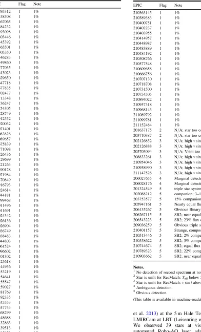
HIRES Follow-up Observations
EPIC Flag Note
201295312 1 1%
201338508 1 1%
201367065 1 1%
201384232 1 1%
201393098 1 1%
201403446 1 1%
201445392 1 1%
201465501 1 1%
201505350 1 1%
201546283 1 1%
201549860 1 1%
201577035 1 1%
201613023 1 1%
201629650 1 1%
201647718 1 1%
201677835 1 1%
201702477 1 1%
201713348 1 1%
201736247 1 1%
201754305 1 1%
201828749 1 1%
201912552 1 1%
201920032 1 1%
202071401 1 1%
202083828 1 1%
202089657 1 1%
202675839 1 1%
203771098 1 1%
203826436 1 1%
204129699 1 1%
204221263 1 1%
204890128 1 1%
205071984 1 1%
205570849 1 1%
205916793 1 1%
205924614 1 1%
205944181 1 1%
205999468 1 1%
206011496 1 1%
206011691 1 1%
206024342 1 1%
206026136 1 1%
206026904 1 1%
206036749 1 1%
206038483 1 1%
206044803 1 1%
206061524 1 1%
206096602 1 1%
206101302 1 1%
206125618 1 1%
206144956 1 1%
206153219 1 1%
206154641 1 1%
206155547 1 1%
206159027 1 1%
206181769 1 1%
206192335 1 1%
206245553 1 1%
206247743 1 1%
206268299 1 1%
206348688 1 1%
206432863 1 1%
206439513 1 1%
206495851 1 1%
Table 3 (Continued)
EPIC Flag Note
210363145 1 1%
210389383 1 1%
210400751 1 1%
210402237 1 1%
210403955 1 1%
210414957 1 1%
210448987 1 1%
210483889 1 1%
210484192 1 1%
210508766 1 1%
210577548 1 1%
210609658 1 1%
210666756 1 1%
210707130 1 1%
210718708 1 1%
210731500 1 1%
210754505 1 1%
210894022 1 1%
210957318 1 1%
210968143 1 1%
211089792 1 1%
211099781 1 1%
211152484 1 1%
201637175 2 N/A; star too cool 203710387 2 N/A; star too cool 202126852 3 N/A; highvsini
202126888 3 N/A; highvsini
205703094 3 N/A; Vsini too high 208833261 3 N/A; highvsini
210954046 3 N/A; highvsini
210958990 3 N/A; highvsini
211147528 3 N/A; highvsini
206027655 4 Marginal detection of 5% binary at−10 kms−1. 206028176 4 Marginal detection at 10 kms−1separation 201324549 5 triple star system; 20% brightness̃
202088212 5 companion; 3–13% as bright as primary; 25 kms−1. 203753577 5 15% companion at 16 kms−1separation
205947161 5 Nearly equalflux binary
206135267 5 Obvious Binary; 50%flux of primary 206267115 5 SB2; near equal at 80 kms−1 206543223 5 SB2; 23%flux of primary 209036259 5 Obvious triple system. 210401157 5 Strange, composite spectrum.
210513446 5 SB2; 2% companion at del-RV=122 kms−1 210558622 5 SB2; 3% companion at del-RV=119 kms−1 210744674 5 SB2; equalflux secondary
210789323 5 SB2; 22% companion at del-RV=−83 kms−1 210903662 5 SB2; near equal binary
Notes.
1No detection of second spectrum at notedflux ratio. 2
Star is unfit for ReaMatch:Teffbelow 3500 K. 3
Star is unfit for ReaMatch:vsiniabove 10 km s−1. 4
Ambiguous detection. 5
Obvious detection.
data were acquired and reduced separately using the standard Robo-AO procedures outlined by Law et al.(2014).
We acquired the data from all our large-aperture AO observations (NIRC2, NIRI, LMIRCam, PHARO) in a consistent manner. We observed at up to nine dither positions, using integration times short enough to avoid saturation (typically60 s). We use the dithered images to remove sky background and dark current, and then align, flat-field, and stack the individual images.
Through our Long-Term Gemini program we also acquired high-resolution speckle imaging of 32 systems in narrowband
filters centered at 692 and 880 nm using the DSSI camera (Horch et al.2009,2012)at the Gemini North telescope. The DSSI observing procedure is typically to center the target star in the field, set up guiding, and take data using 60 ms exposures. The total integration time varies by target brightness and observing conditions. We measure background sensitivity in a series of concentric annuli around the target star. The innermost data point represents the telescope diffraction limit, within which we set our sensitivity to zero. After measuring our sensitivity across the DSSI field of view, we interpolate through the measurements using a cubic spline to produce a smooth sensitivity curve.
3.3.2. Contrast and Stellar Companions
We estimate the sensitivity of all our HRI data by injecting fake sources into thefinal combined images with separations at integral multiples of the central source’s FWHM (see, e.g., Adams et al. 2012; Ziegler et al. 2016). Figure 4 shows an example of a Keck/NIRC2 NGS image and the resulting 5σ contrast curve. The median contrast curves achieved by each HRI instrument are shown in Figure5together with all detected stellar companions. The companions are also listed in Table5. Contrast curves for each individual system are uploaded to the ExoFOP website. In addition, Table 10 includes the total integration times andfilters used for all candidates observed in our follow-up efforts.
[image:7.612.48.297.74.727.2] [image:7.612.316.568.76.260.2]The contrast curves are plotted in the band of observations, which ranges from optical wavelengths (DSSI; Robo-AO) to the K-band (large-aperture AO systems). These in-band
Table 4
FEROS Radial Velocities
EPIC BJD RV sRV tint S/N
203294831 2457182.56854355 6.235 0.093 600 45
203771098 2457182.57744262 0.713 0.010 600 82
201176672 2457182.58920619 41.702 0.029 1800 25
201626686 2457182.62251241 49.133 0.015 600 49
203929178 2457182.67319105 −130.200 0.221 600 54
203771098 2457183.50141524 0.725 0.010 600 78
203929178 2457183.53736243 64.251 0.276 600 51
201626686 2457183.54133676 49.090 0.011 600 76
204873331 2457183.74219492 48.694 0.620 900 46
203485624 2457183.75453967 93.324 1.867 900 47
203294831 2457183.76528655 7.172 0.076 600 46
205148699 2457183.77680036 −41.853 0.058 900 43
203294831 2457184.51873516 6.106 0.118 600 34
204873331 2457184.54186421 −39.425 0.559 900 43
205148699 2457184.55524152 −32.892 0.055 900 46
203771098 2457184.57256456 0.707 0.010 600 90
203929178 2457184.58722675 −80.916 0.226 600 57
203485624 2457184.70016264 −8.811 1.983 900 54
201176672 2457185.53558417 41.739 0.023 1800 31
201626686 2457185.55294623 49.105 0.011 600 74
203294831 2457185.61605114 6.799 0.076 600 43
203929178 2457185.67144651 −3.928 0.841 600 53
205148699 2457185.68276227 −61.542 0.055 900 45
204873331 2457185.76186667 −51.492 0.320 900 53
203485624 2457185.77667465 −58.772 3.136 900 39
203485624 2457186.59017442 −20.641 1.277 900 40
205148699 2457186.60319043 −77.486 0.068 900 35
205148699 2457186.61615822 −77.408 0.060 900 41
204873331 2457186.62889121 6.458 0.327 900 35
203929178 2457186.68052468 −20.963 0.161 600 44
203294831 2457186.80984085 5.598 0.121 600 37
203929178 2457187.61615918 −76.018 0.467 600 59
203485624 2457187.62722491 −121.651 2.046 900 52
201626686 2457190.49169087 49.070 0.010 600 80
203485624 2457190.57993074 −17.006 1.498 900 58
203294831 2457190.59359013 5.611 0.072 600 61
203294831 2457191.51831070 5.522 0.083 600 50
203485624 2457191.53066007 69.097 1.920 900 3
203929178 2457191.54262838 −88.136 0.276 600 53
204873331 2457191.55366638 42.413 0.630 900 36
201176672 2457192.52186285 41.755 0.026 1800 26
201626686 2457192.54283939 49.094 0.015 600 46
203294831 2457192.56384913 1.127 0.770 600 21
201626686 2457193.51718740 49.149 0.015 600 49
203294831 2457193.53338541 5.362 0.113 600 36
203485624 2457193.54441500 −62.799 1.150 900 35
204873331 2457193.56058533 −39.060 0.228 900 62
205148699 2457193.57490799 −38.108 0.048 900 54
203929178 2457193.74554128 −27.479 0.915 600 62
201176672 2457194.51197780 41.713 0.022 1800 32
201626686 2457194.52827067 49.060 0.011 600 73
203929178 2457194.54604512 −78.496 0.263 600 63
203485624 2457194.57421092 40.485 2.366 900 40
203294831 2457194.58577034 2.920 0.183 600 50
203771098 2457194.59578556 0.720 0.010 600 97
205148699 2457194.60718775 −65.417 0.047 900 55
204873331 2457194.76473872 −30.284 0.301 900 42
203485624 2457195.57768234 −30.056 3.353 900 43
203929178 2457195.59152469 62.791 0.432 600 40
204873331 2457195.60248537 51.545 0.467 900 41
205148699 2457195.61518621 −78.246 0.073 900 33
203294831 2457195.67227197 2.509 0.482 600 21
203771098 2457195.68202812 0.683 0.015 600 32
203294831 2457211.65688105 4.917 0.081 600 43
Table 4 (Continued)
EPIC BJD RV sRV tint S/N
203929178 2457211.67035362 74.751 0.344 600 55
203771098 2457211.68015495 0.722 0.010 600 95
203485624 2457211.69331295 42.800 6.707 900 41
204873331 2457211.70909075 0.643 0.274 900 54
205148699 2457211.72234337 −56.025 0.047 900 53
201626686 2457218.47908419 49.071 0.012 900 60
201626686 2457219.46201643 49.100 0.013 600 57
201626686 2457220.48312511 49.054 0.013 600 57
201626686 2457221.48191204 49.087 0.012 600 69
202088212 2457408.67412585 −17.112 0.021 900 87
201505350 2457409.82308403 7.334 0.011 1500 45
201270176 2457410.85912543 91.924 0.088 1100 37
201862715 2457410.87002659 13.448 0.010 420 69
201505350 2457412.79619955 7.369 0.011 1500 47
201862715 2457412.84747439 13.645 0.010 420 75
201270176 2457413.72138662 80.691 0.064 1100 52
magnitude differences set upper limits on the maximum amount of blending possible within the Kepler bandpass. If the companion has the same color as the primary, then the measuredΔmag is indeed theΔKp. If the companion is redder, then the Kp-band flux ratio is even smaller. All detected sources are included in Table5, even though some lie outside of our photometric apertures. In these cases the detected companion has little or no impact on the transit parameters and FPPs derived below. We discuss such considerations more thoroughly in Section6.2.
4. STELLAR PARAMETERS
[image:8.612.44.581.38.741.2] [image:8.612.47.317.67.726.2] [image:8.612.314.567.80.525.2]Stellar parameters are needed to convert the physical properties measured by our transit photometry into useful planetary parameters such as radius (RP) and incident Table 5
HRI-detected Stellar Companions
EPIC rap ρ Delta mag Filter Telescope
(″) (″) (mag)
201176672 11.94 0.340 2.77 K Keck2
201295312 11.94 8.110 4.00 K Keck2
201295312 11.94 8.070 4.10 K Palomar
201324549 11.94 0.090 0.43 K GemN-NIRI
201488365 L 4.100 9.56 i Robo-AO
201505350 11.94 0.160 0.36 K Palomar
201546283 7.96 3.030 5.83 i Robo-AO
201546283 7.96 2.960 3.74 K Keck2
201626686 11.94 15.390 2.43 K Palomar
201629650 11.94 3.210 5.79 K Keck2
201828749 11.94 2.540 1.97 i Robo-AO
201828749 11.94 2.450 1.07 K Keck2
201828749 11.94 2.440 1.11 K Palomar
201862715 11.94 1.450 0.90 i Robo-AO
201862715 11.94 1.470 0.51 K Palomar
202059377 11.94 0.390 0.34 i Robo-AO
202059377 11.94 0.360 0.32 K LBT
202066212 L 9.120 0.43 K Palomar
202066212 L 10.580 2.72 K Palomar
202066537 7.96 2.280 0.69 i Robo-AO
202066537 7.96 2.290 0.58 K LBT
202071289 11.94 0.060 0.09 K Keck2
202071401 15.92 2.880 2.49 i Robo-AO
202071401 15.92 6.230 5.05 i Robo-AO
202071401 15.92 2.840 1.70 K Keck2
202071401 15.92 2.840 1.79 K Palomar
202071401 15.92 6.050 5.23 K Palomar
202071645 11.94 3.700 7.19 i Robo-AO
202071645 11.94 3.360 7.06 K Palomar
202071645 11.94 3.630 7.43 K Palomar
202071645 11.94 9.290 3.67 K Palomar
202071645 11.94 10.850 5.88 K Palomar
202083828 11.94 5.530 5.02 i Robo-AO
202088212 15.92 1.310 6.79 K Keck2
202089657 15.92 8.550 5.28 K Palomar
202089657 15.92 9.210 5.58 K Palomar
202089657 15.92 11.160 4.67 K Palomar
202089657 15.92 11.630 6.73 K Palomar
202126849 15.92 4.610 5.70 i Robo-AO
202126852 15.92 7.150 7.44 K Palomar
202126852 15.92 3.730 6.99 K Palomar
202126852 15.92 7.170 7.38 i Robo-AO
202126887 15.92 5.770 2.79 i Robo-AO
202126887 15.92 7.260 2.33 i Robo-AO
202126887 15.92 5.580 2.53 K Keck2
202126887 15.92 7.200 1.41 K Keck2
202126888 15.92 6.700 5.98 i Robo-AO
202565282 7.96 2.170 5.19 K Keck2
203929178 19.9 0.110 1.37 K Keck2
204043888 7.96 5.520 4.73 K Keck2
204489514 15.92 5.390 4.49 K Keck2
204890128 15.92 7.510 1.55 K Keck2
205029914 11.94 3.320 0.87 K Keck2
205064326 11.94 4.270 3.92 K Keck2
205148699 11.94 0.090 0.83 K Keck2
205686202 11.94 0.790 3.82 K Keck2
205703094 11.94 0.140 0.37 K Keck2
205916793 11.94 7.300 0.35 K Palomar
205962680 11.94 0.480 0.27 K Keck2
205999468 7.96 18.500 3.27 K Palomar
206011496 7.96 0.980 2.81 K Keck2
206047297 11.94 9.560 5.90 K Palomar
206061524 7.96 0.410 1.37 K Palomar
Table 5 (Continued)
EPIC rap ρ Delta mag Filter Telescope
(″) (″) (mag)
206192335 11.94 2.240 6.18 K GemN-NIRI
206192335 11.94 2.260 6.21 K Palomar
207389002 11.94 5.940 2.36 K GemS-GNIRS
207389002 11.94 5.370 2.96 K GemS-GNIRS
207389002 11.94 5.910 2.29 i Robo-AO
207475103 15.92 0.100 0.12 K LBT
207475103 15.92 4.340 3.18 i Robo-AO
207475103 15.92 7.610 −2.11 i Robo-AO
207475103 15.92 7.700 2.51 i Robo-AO
207517400 15.92 3.530 2.63 i Robo-AO
207517400 15.92 3.430 1.92 K Palomar
207517400 15.92 8.320 1.35 K Palomar
207517400 15.92 10.620 −2.12 K Palomar
207739861 11.94 5.440 1.62 i Robo-AO
208445756 11.94 5.970 1.37 i Robo-AO
208445756 11.94 5.850 1.19 K Palomar
208445756 11.94 11.290 3.06 K Palomar
208445756 11.94 13.130 3.79 K Palomar
208445756 11.94 12.000 4.05 K Palomar
209036259 15.92 4.000 2.96 i Robo-AO
210401157 5.572 0.500 2.47 a GemN-Spk
210401157 5.572 0.490 2.27 b GemN-Spk
210401157 5.572 0.470 1.67 K Keck2
210414957 15.92 0.790 2.41 K GemN-NIRI
210414957 15.92 1.020 4.95 K GemN-NIRI
210513446 7.96 0.240 1.26 K GemN-NIRI
210666756 5.572 2.360 1.30 K GemN-NIRI
210666756 5.572 7.850 1.28 K GemN-NIRI
210769880 15.92 0.780 5.39 K GemN-NIRI
210954046 7.96 2.930 1.45 K GemN-NIRI
210958990 11.94 1.740 2.52 a GemN-Spk
210958990 11.94 1.790 2.80 b GemN-Spk
210958990 11.94 1.820 1.71 K Keck2
211089792 15.92 4.240 0.89 K GemN-NIRI
211147528 15.92 1.330 6.75 b GemN-Spk
211147528 15.92 1.300 5.02 K Keck2
203099398 L 1.970 1.67 K Keck2
203867512 L 0.453 0.61 K Keck2
204057095 L 0.790 2.71 K Keck2
204057095 L 0.870 2.97 K Keck2
204750116 L 2.980 5.91 K Keck2
irradiation(Sinc). We use several complementary techniques to
infer stellar parameters for our entire sample.
For all stars with Keck/HIRES and/or APF/Levy spectra, we attempt to estimate effective temperatures, surface gravities, metallicities, and rotational velocities using SpecMatch (Petigura 2015). SpecMatch fits a high-resolution optical spectrum to an interpolated library of model spectra from Coelho et al.(2005), which closely match the spectra of well-characterized stars in this temperature range. Uncertainties on
Teff, logg, and [Fe/H] from HIRES spectra are 60 K,
0.08–0.10 dex, and 0.04 dex, respectively (Petigura 2015).
Experience shows that SpecMatch is limited to stars with
Teff∼4700–6500K andvsini30kms−1.
TheSpecMatchpipeline used to analyze the APF data is identical to the KeckSpecMatchpipeline, except we employ the differential-evolution Markov Chain Monte Carlo ( DE-MCMC; Ter Braak 2006) fitting engine from ExoPy (Fulton et al.2013)instead ofc2minimization. The APFSpecMatch
pipeline was empirically calibrated to produce consistent stellar parameters for stars that were observed at both Keck and APF by fitting and subtracting a three-dimensional surface to the residuals ofTeff,logg, and Fe/H between the calibrated Keck
[image:9.612.322.564.51.235.2]and initial APF parameters. The errors on the stellar parameters are a quadrature sum of the statistical errors from the DE-MCMCfits and the scatter in the APF versus Keck calibration. The scatter in the calibration is generally an order of magnitude
Table 6
Disposition of Multi-star Candidates
EPIC r<4″ F F2 1< ¢d Comment
201176672 True True Cannot validate candidate. 201295312 False True Same depth forr=1″aperture. 201324549 True True Cannot validate candidate. 201546283 True True Cannot validate candidate. 201626686 False True Shallower transit withr=1″;
likely FP.
201629650 True True Cannot validate candidate. 201828749 True True Cannot validate candidate. 201862715 True True Cannot validate candidate. 202059377 True True Cannot validate candidate. 202066537 True True Cannot validate candidate. 202071289 True True Cannot validate candidate. 202071401 True True Cannot validate candidate. 202071645 True False Secondary star sufficiently faint. 202083828 False True Same depth forr=1″aperture. 202088212 True False Secondary star sufficiently faint. 202126849 False False Secondary star sufficiently faint. 202126852 False False Secondary star sufficiently faint. 202126887 False True Deeper transit withr=1″aperture. 202126888 False True Same depth forr=1″aperture. 202565282 True False Secondary star sufficiently faint. 203929178 True True Cannot validate candidate. 204043888 False False Secondary star sufficiently faint. 204489514 False False Secondary star sufficiently faint. 204890128 False True Same depth forr=1″aperture. 205029914 True True Cannot validate candidate. 205064326 False True Shallower transit withr=1″;
likely FP.
[image:9.612.44.292.73.591.2]205148699 True True Cannot validate candidate. 205686202 True True Cannot validate candidate. 205703094 True True Cannot validate candidate. 205916793 False True Deeper transit withr=1″aperture. 205999468 False True Same depth forr=1″aperture. 206011496 True True Cannot validate candidate. 206061524 True True Cannot validate candidate. 206192335 True True Cannot validate candidate. 207389002 False False Secondary star sufficiently faint. 207475103 True True Cannot validate candidate. 207517400 True True Cannot validate candidate. 207739861 False True Cannot validate candidate. 208445756 False True Cannot validate candidate. 209036259 False True Cannot validate candidate. 210401157 True True Cannot validate candidate. 210414957 True True Cannot validate candidate. 210513446 True True Cannot validate candidate. 210666756 True True Cannot validate candidate. 210958990 True True Cannot validate candidate. 211089792 False True Same depth forr=1″aperture. 211147528 True True Cannot validate candidate.
Figure 4.Example constraints on any additional, nearby stars around K2-77
(EPIC 210363145)from Keck/NIRC2 K-band adaptive optics imaging. For this target, no companions were detected above the plotted contrast limits. Detected stellar companions around all observed candidates are listed in Table5.
Figure 5. Stellar companions (triangles) detected near our K2 candidate systems and the median contrast achieved with each listed instrument andfilter
[image:9.612.323.565.308.496.2]larger than the statistical errors in the S/N regime for the K2
targets observed on APF.
Petigura (2015) assessed the accuracy of SpecMatch -derived stellar parameters by modeling the spectra of several samples of touchstone stars with well-measured properties. The properties of these stars were determined from asteroseismol-ogy (Huber et al.2012), detailed LTE spectral modeling, and transit light curve modeling (Torres et al.2012), and detailed LTE spectral modeling (Valenti & Fischer 2005). The uncertainties of SpecMatch parameters are dominated by errors in the Coelho et al. (2005) model spectra (e.g., inaccuracies in the line lists, assumption of LTE, etc.). Given that we observe spectra at S/N35 per pixel, photon-limited errors are not an appreciable fraction of the overall error budget.
To estimate stellar masses and radii for all stars with
SpecMatch parameters, we use the free and open source
isochrones Python package (Morton 2015a). This tool accepts as inputs the Teff, logg, and [Fe H] measured by SpecMatch and interpolates over a grid of stellar models from the Dartmouth Stellar Evolution Database (Dotter et al. 2008). isochrones uses the emcee Markov Chain Monte Carlo package (Foreman-Mackey et al. 2012) to estimate uncertainties, sometimes reporting fractional uncer-tainties as low as 1%. Following Sinukoff et al. (2016), we adopt a lower limit of 5% for the uncertainties on stellar mass and radius to account for the intrinsic uncertainties of the Dartmouth models found by Feiden & Chaboyer (2012).
Eighty-five stars in our sample lack SpecMatch para-meters. For most of these, we adopt the stellar parameters of Huber et al.(2016). This latter analysis relies on the Padova set of stellar models (Marigo et al. 2008), which systematically underestimate the stellar radii of low-mass stars. Follow-up spectroscopy to provide refined parameters for these later-type stars is underway (C. Dressing et al. 2016, in preparation; A. Martinez et al. 2016, in preparation). Our sample includes a small number of stars not considered by Huber et al. (2016), such as targets in K2’s Campaign 0. For these, we use
isochrones in conjunction with broadband photometry collected from the APASS, 2MASS, andWISEsurveys to infer the stellar parameters.
We then use the free, open sourceLDTktoolkit(Parviainen & Aigrain2015)to propagate our measuredTeff,logg,[Fe/H],
and their uncertainties into limb-darkening coefficients and associated uncertainties. These limb-darkening parameters act as priors in our transit light curve analysis(described below in Section 5). We upgraded LDTk to allow the (typically non-Gaussian) posterior distributions generated by the
iso-chrones package to be fed directly into the limb-darkening analysis.40 Because LDTk often reports implausibly small uncertainties on the limb-darkening parameters, based on our experience with such analyses we increase all these uncertain-ties by a factor offive in our light curve analyses. Spot checks of a number of systems reveal that imposing priors on the stellar limb-darkening has a negligible impact (<1σ) on our
final results, relative to analyses with much weaker constraints on limb darkening.
All our derived stellar parameters—Teff,logg,R,M—and
their uncertainties are listed in Table 7.
5. TRANSIT LIGHT CURVE ANALYSES
After identifying planet candidates and determining the parameters of their host stars, we subject the detrended light curves to a full maximum-likelihood and MCMC analysis. We use a custom Python wrapper of the free, open sourceBATMAN light curve code(Kreidberg2015). We upgraded theBATMAN codebase to substantially increase its efficiency when analyzing long-cadence data.41The light curves arefit using the standard Nelder-Mead Simplex Algorithm42 and then run through
emceeto determine parameter uncertainties.
Our general approach follows that used in our previous papers(Crossfield et al. 2015; Petigura et al.2015; Schlieder et al.2016; Sinukoff et al.2016). The model parameters in our analysis are the transit time(T0); the candidate’s orbital period
and inclination(Pandi); the scaled semimajor axis(a R*); the fractional candidate size (R Rp *); the orbital eccentricity and
longitude of periastron(eandω), the fractional level of dilution (δ) from any other sources in the aperture; a single multi-plicative offset for the absoluteflux level; and quadratic limb-darkening coefficients (u1and u2). We initialize eachfit with
the best-fit parameters returned from TERRA. Note that both this analysis and that ofTERRAassume a linear ephemeris, so systems with large transit timing variations (TTVs) could be missed or misidentified.
During the analysis, several parameters are constrained or subjected to various priors. Gaussian priors are applied to the limb-darkening parameters (as derived from the LDTk analysis), toP(with a dispersion ofsP=0.01 days, to ensure
that the desired candidate signal is the one being analyzed), and toe(me=10-4andse=10-3, to enforce a circular orbit). We
also apply a uniform prior toT0(with width0.06P),i(from 50°
to 90°),R Rp *(from−1 to 1), andω(from 0 to 2π); bothPand
*
a R are furthermore constrained to be positive. Allowing *
RP R to take on negative values avoids the Malmquist bias
that would otherwise result from treating it as a positive-definite quantity. For those systems with no identified stellar companions, our HRI and/or spectroscopy constrain the dilution level; otherwise, we adopt a log-uniform prior on the interval(10−6, 1).
6. FALSE POSITIVE ASSESSMENT
During the primeKeplermission, both the sheer number of planet candidates and their intrinsic faintness made direct confirmation by RVs impractical for most systems. Nonetheless many planets can be statistically validated by assessing the relative probabilities of planetary and false positive scenarios; a growing number of groups have presented frameworks for quantitatively assessing the likelihoods of planetary and false positive scenarios (Torres et al. 2011; Morton 2012; Díaz et al.2014; Santerne et al.2015). These false positive scenarios come in several classes: (1) undiluted eclipsing binaries, (2) background (and foreground) eclipsing binaries where the eclipses are diluted by a third star, and(3)eclipsing binaries in gravitationally bound triple systems.
To estimate the likelihood that each of our planet candidates is a true planetary system or a false positive configuration, we use the free and open sourcevespasoftware(Morton2015).
vespa compares the likelihood of each scenario against the planetary interpretation and accepts additional constraints from
40
GitHub commits 60174cc, 46d140b, and 8927bc6.
41
GitHub commit 9ae9c83. 42
HRI and spectroscopy. Throughout this analysis, we apply Version 0.4.7 ofvespa(using the MultiNest backend)to each individual planetary candidate. Other types of false positive scenarios exist that are not explicitly treated byvespa, such as eclipsing binaries on eccentric, inclined orbits showing only transit or occultation(but not both), or extremely inconvenient arrangements of starspots. The community’s experience of following up transiting planet candidates indicates that such scenarios are much less common than those considered by
vespa; nonetheless quantifying the likelihood of such scenarios for each candidate would be an interesting avenue for future research.
6.1. Calculating FPPs
To calculate the FPP for each system, we use the following inputs: stellar photometry from APASS, 2MASS, and WISE; the stellar parameters described in Section 4; the detrended light curve (after masking out any transits from other candidates in that system); the exclusion constraints from adaptive optics imaging data in terms of contrast versus separation (where available) and from our high-resolution spectroscopy (maximum allowed contrast and velocity offset); and an upper limit on the depth of any secondary eclipse. We derive the last of these by constructing a rectangular signal with depth unity and duration equal to the best-fit transit duration, scanning the template signal across the out-of-transit light curve, and reporting the 99.7th percentile as the eclipse depth’s upper limit.
We report thefinal FPPs of all our systems in Table8. For the purposes of the discussion that follows, we deem any candidate signal with FPP<0.01 as a validated extrasolar planet and signals with FPP>0.99 as false positives. For all unvalidated candidates, Table9summarizesvespaʼs estimate of the relative(unnormalized)likelihood of each potential false positive scenario.
The vespa algorithm implicitly assumes that each planet candidate lacks any other companion candidates in the same system. Studies of Kepler’s multiple-candidate systems show that almost all are planets (Lissauer et al. 2012). This “multiplicity boost” has subsequently been used to validate hundreds of multi-planet systems(Rowe et al.2014). Because
vespatreats only single-planet systems, we simply treat these multi-candidate systems as independent, isolated candidates in
the FPP analysis. Sinukoff et al. (2016) show that K2’s multiplicity boost is 20 even in crowdedfields, comparable to the boost factor derived for the originalKeplermission.
Even without the multiplicity boost, our approach validates the majority of our multi-candidate systems. Both EPIC201445392(K2-8)and EPIC206101302 host two-planet candidates. In each system we validate one candidate andfind FPP=4%–7% for the other. The K2multiplicity boost factor of 20 therefore results in all candidates in both systems being
firmly labeled as validated planets.
A more complicated case is EPIC205703094, which hosts three planet candidates. Our vespa analysis finds that one candidate is a false positive and that the others both have FPP≈50%(see Tables8and9). Our light curve analysisfinds that all three candidates are well-fit by grazing transits(b ~1), leavingRP R*only weakly constrained. Furthermore, our HRI
reveals that the system is a close visual binary with separation 0 14(see Tables6 and 5). Therefore we can neither validate nor rule out the three candidates in this system.
6.2. Targets with Nearby Stellar Companions
Planet candidates orbiting stars in physical or visual multiple systems are much more difficult to validate due to blending in the photometric aperture(see, e.g., Ciardi et al.2015). Table5
shows that ourK2photometric apertures are quite large(up to 20″ in extreme cases) and that HRI follow-up reveals stellar companions within these apertures for many systems. There-fore we must treat these systems with greater care.
To demonstrate the difficulty, consider two stars with flux ratioF F2 1<1and angular separationρ. Assume both lie in a
photometric aperture with radiusr>r, with which a transit is observed with apparent depthδ′. If the transit occurs around the primary star, then the true transit depth isd1» ¢d (1 -F F2 1);
this is at most twice the observed depth, indicating a planetary radius up to 2 larger than otherwise determined. If instead the transiting object orbits the secondary, then the true transit depth isd2» ¢dF F1 2 and the transiting object may be many times
larger than expected. Table6lists all candidates known to host secondary stars and their relationships betweenF F2 1&d¢and
ρ&r.
Any planet candidate in a multi-star system and with d
< ¢
F F2 1 cannot transit the secondary(which is too faint to
[image:11.612.42.573.74.217.2]be the source of the observed transit signal). We find several
Table 7
Stellar Parameters
EPIC Kp R* M* Teff logg Source
(mag) (R) (M) (K) (dex)
201155177 14.632 0.643(39) 0.702(46) 4613(71) 4.659(50) Huber et al.(2016)
201176672 13.980 0.508(98) 0.559(87) 4542(130) 4.747(97) Huber et al.(2016)
201205469 14.887 0.570(30) 0.600(30) 3939(87) 4.698(23) Huber et al.(2016)
201208431 14.409 0.435(60) 0.487(72) 4044(81) 4.849(60) Huber et al.(2016)
201247497 16.770 0.436(27) 0.492(29) 3918(46) 4.846(50) Huber et al.(2016)
201295312 12.126 1.58(15) 1.150(60) 5912(51) 4.101(63) SpecMatch
201324549 12.146 1.45(25) 1.18(12) 6283(113) 4.17(12) Huber et al.(2016)
201338508 14.364 0.462(38) 0.520(44) 4021(62) 4.823(50) Huber et al.(2016)
201345483 15.319 0.445(66) 0.503(78) 4103(90) 4.824(70) Huber et al.(2016)
201367065 11.574 0.371(50) 0.414(58) 3841(82) 4.906(60) Huber et al.(2016)
201384232 12.510 1.010(80) 0.930(30) 5767(58) 4.398(74) SpecMatch
Table 8
Planet Candidate Parameters
Other EPIC P T0 T14 RP R* a RP Sinc FPP Disposition
Name (d) (BJDTDB (hr) (%) (au) (R⊕) (S⊕)
–2454833)
K2-42b 201155177.01 6.68796(93) 1981.6763(52) 3.04(20) 3.04(28) 0.0617(13) 2.15(24) 44.1(6.3) 5.2e−07 Planet
201176672.01 79.9999(98) 2044.8046(15) 11.75(17) 18.0(1.1) 0.299(16) 10.2(2.1) 1.10(46) 0.094 Candidate(see Tables6and1)
K2-43b 201205469.01 3.47114(21) 1976.8845(33) 1.97(11) 6.60(36) 0.03784(63) 4.13(31) 49.0(6.9) 9.7e−10 Planet K2-4b 201208431.01 10.0044(11) 1982.5170(45) 2.87(17) 3.49(41) 0.0715(35) 1.69(30) 8.9(2.7) 0.00028 Planet
201247497.01 2.75391(15) 1977.9031(23) 1.03(14) 7.9(1.3) 0.03035(59) 3.78(68) 43.7(6.1) 0.41 Candidate K2-44b 201295312.01 5.65688(59) 1978.7176(44) 4.36(13) 1.56(12) 0.0651(11) 2.72(32) 646(126) 6.7e−07 Planet
201324549.01 2.519334(35) 1976.99353(69) 1.545(15) 2.41(30) 0.0383(13) 3.91(85) 2002(727) 1 False Positive(see Tables6and3)
K2-5c 201338508.01 10.9324(14) 1981.6012(55) 2.84(23) 3.24(29) 0.0775(22) 1.64(20) 8.3(1.6) 2.8e−05 Planet K2-5b 201338508.02 5.73597(68) 1975.8602(53) 2.35(18) 2.97(22) 0.0504(14) 1.50(17) 19.7(3.7) 5.4e−06 Planet K2-45b 201345483.01 1.7292684(69) 1976.52604(18) 1.689(14) 13.76(19) 0.0224(12) 6.71(00) 100(32) 6.8e−06 Planet K2-3b 201367065.01 10.05443(26) 1980.4178(12) 2.520(59) 3.51(15) 0.0679(32) 1.44(20) 5.8(1.7) 1.9e−08 Planet K2-3c 201367065.02 24.6435(12) 1979.2811(24) 3.38(12) 2.88(16) 0.1235(58) 1.18(17) 1.77(53) 2.1e−08 Planet K2-3d 201367065.03 44.5609(52) 1993.2285(34) 4.04(19) 2.35(15) 0.1833(86) 0.96(14) 0.80(24) 1.2e−07 Planet
Note.Table8is published in its entirety in the machine-readable format. A portion is shown here for guidance regarding its form and content.
(This table is available in its entirety in machine-readable form.)
12
Astrophysical
Journal
Supplement
Series,
226:7
(
20pp
)
,
2016
September
Cross
fi
eld
et
such systems, though only two (EPIC 202126852 and 211147528) have FPP<0.95. Nonetheless, for all these systems we account for the dilution of the secondary star(s) as described below.
For candidates withd¢ < F F2 1andr<r, the transit could
[image:13.612.52.573.76.606.2]occur around either star. We compare our nominal time-series photometry to that computed with r=1 pixel for all such candidates. For targets with more widely separated nearby
Table 9
Unvalidated Candidate False Positive Likelihoods
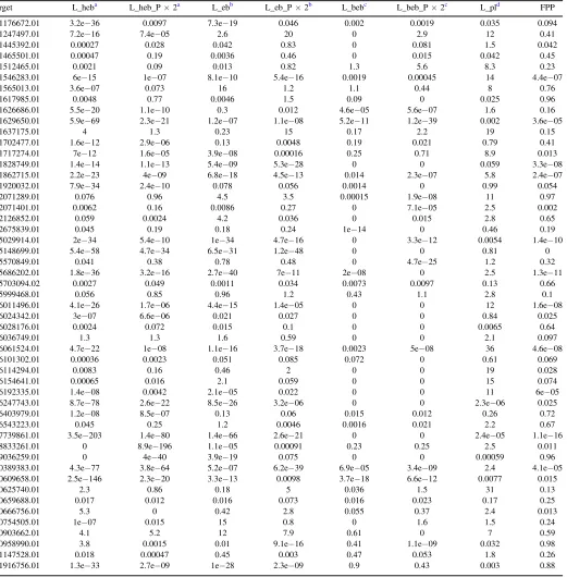
Target L_heba L_heb_P×2a L_ebb L_eb_P×2b L_bebc L_beb_P×2c L_pld FPP
201176672.01 3.2e−36 0.0097 7.3e−19 0.046 0.002 0.0019 0.035 0.094
201247497.01 7.2e−16 7.4e−05 2.6 20 0 2.9 12 0.41
201445392.01 0.00027 0.028 0.042 0.83 0 0.081 1.5 0.042
201465501.01 0.00047 0.19 0.0036 0.46 0 0.015 0.042 0.45
201512465.01 0.0021 0.09 0.013 0.82 1.3 5.6 8.3 0.23
201546283.01 6e−15 1e−07 8.1e−10 5.4e−16 0.0019 0.00045 14 4.4e−07
201565013.01 3.6e−07 0.073 16 1.2 1.1 0.44 8 0.76
201617985.01 0.0048 0.77 0.0046 1.5 0.09 0 0.025 0.96
201626686.01 5.5e−20 1.1e−10 0.3 0.012 4.6e−05 5.6e−07 1.6 0.16
201629650.01 5.9e−69 2.3e−21 1.2e−07 1.1e−08 5.2e−11 1.2e−39 0.002 3.6e−05
201637175.01 4 1.3 0.23 15 0.17 2.2 19 0.15
201702477.01 1.6e−12 2.9e−06 0.13 0.0048 0.19 0.021 0.79 0.41
201717274.01 7e−12 1.6e−05 3.9e−08 0.00016 0.25 0.71 8.9 0.013
201828749.01 1.4e−14 1.1e−13 5.4e−09 5.3e−28 0 0 0.059 3.3e−08
201862715.01 2.2e−23 4e−09 6.8e−18 4.5e−13 0.014 2.3e−07 5.8 2.4e−07
201920032.01 7.9e−34 2.4e−10 0.078 0.056 0.0014 0 0.99 0.054
202071289.01 0.076 0.96 4.5 3.5 0.00015 1.9e−08 11 0.97
202071401.01 0.0062 0.16 0.0086 0.27 0 7.1e−05 2.5 0.002
202126852.01 0.059 0.0024 4.2 0.036 0 0.015 2.8 0.65
202675839.01 0.045 0.19 0.18 0.24 1e−14 0 0.46 0.19
205029914.01 2e−34 5.4e−10 1e−34 4.7e−16 0 3.3e−12 0.0054 1.4e−10
205148699.01 5.4e−58 4.7e−34 6.5e−31 1.2e−48 0 0 0.81 0
205570849.01 0.041 0.38 0.78 0.48 0 4.7e−25 1.2 0.32
205686202.01 1.8e−36 3.2e−16 2.7e−40 7e−11 2e−08 0 2.5 1.3e−11
205703094.02 0.0027 0.049 0.0011 0.034 0.0073 0.0097 0.13 0.66
205999468.01 0.056 0.85 0.96 1.2 0.43 1.1 2.8 0.1
206011496.01 4.1e−26 1.7e−06 4.4e−15 1.4e−05 0 0 12 1.6e−08
206024342.01 3e−07 6.6e−06 0.021 0.027 0 0 0.84 0.025
206028176.01 0.0024 0.072 0.015 0.1 0 0 0.0065 0.64
206036749.01 1.3 1.3 1.6 0.59 0 0 2.1 0.097
206061524.01 4.7e−22 1e−08 1.1e−16 3.7e−18 0.0023 5e−08 36 4.6e−08
206101302.01 0.00036 0.0023 0.051 0.085 0.072 0 0.61 0.069
206114294.01 0.0083 0.16 0.46 2 0 0 19 0.028
206154641.01 0.00065 0.016 2.1 0.059 0 0 15 0.074
206192335.01 1.4e−08 0.0042 2.1e−05 0.022 0 0 11 6e−05
206247743.01 8.7e−78 2.6e−22 8.5e−26 3.2e−06 0 0 2.3e−06 0.025
206403979.01 1.2e−08 8.5e−07 0.13 0.06 0.015 0.012 0.26 0.72
206543223.01 0.045 0.25 1.2 0.0046 0.0016 0.021 2.2 0.67
207739861.01 3.5e−203 1.4e−80 1.4e−66 2.6e−21 0 0 2.4e−05 1.1e−16
208833261.01 0 8.9e−196 1.1e−05 0.00091 0.23 0.25 2.5 0.011
209036259.01 0 4e−40 3.9e−19 0.075 0 0 0.00059 0.96
210389383.01 4.3e−77 3.8e−64 5.2e−07 6.2e−39 6.9e−05 3.4e−09 2.4 4.1e−05
210609658.01 2.5e−146 2.3e−20 3.3e−13 0.0098 3.7e−18 6.6e−12 0.0077 0.015
210625740.01 2.3 0.86 0.18 5 0.036 1.5 31 0.13
210659688.01 0.017 0.012 0.016 0.073 0.016 0.023 0.17 0.25
210666756.01 5.3 0 0.42 2.8 0.055 0.37 2.4 0.013
210754505.01 1e−07 0.015 15 0.8 0 1.6 1.5 0.24
210903662.01 4.1 5.2 12 7.9 0.61 0 7 0.59
210958990.01 3.8 0.0015 0.01 9.1e−16 0.41 1.1e−09 0.032 0.98
211147528.01 0.018 0.00047 0.45 0.003 0.47 0.053 1.8 0.26
211916756.01 1.3e−33 2.7e−09 1e−28 2.3e−09 0.9 0.43 0.003 0.88
Notes.
a
Likelihood that the system is a hierarchical eclipsing binary, with orbital period either as measured or twice that measured. b
Likelihood that the system is an eclipsing binary, with orbital period either as measured or twice that measured. c
Likelihood that the system is a blended eclipsing binary, with orbital period either as measured or twice that measured. d
Likelihood that the system is a transiting planet.
stars, if the one-pixel-photometry reveals a shallower transit, then the transit probably occurs around the secondary star. However, if r<1pix then we cannot reliably identify the source of the transits. Wefind 28 candidates of these types that we cannot validate at present, and note the disposition of all such systems in Table 6.
For all remaining systems, the detected transits must occur around the primary star but will be diluted by light from the secondary. We estimate the total brightness of these systems’ secondary star(s) as follows. For stars detected by optical imaging(Robo-AO and DSSI), we use the measured contrast ratio with an uncertainty of 0.05mag. For stars detected by infrared imaging, we use the relations of Howell et al.(2012)to translate the observed infrared color into the Keplerbandpass. Since these relations are approximate and depend strongly on SpT, we conservatively apply an uncertainty of 0.5mag to these values. Section 6.2describes how we use these data to constrain the dilution parameter’s posterior distribution, thereby reducing the systematic biases induced by unrecog-nized sources of dilution(e.g., Ciardi et al.2015).
7. RESULTS AND DISCUSSION
Wefind 104 validated planets(i.e., FPP<0.01)in our set of 197 planet candidates. Significantly, we show thatK2’s surveys increase by 30% the number of small planets orbiting moderately bright stars compared to previously known planets. In Section 7.1 we present a general overview of our survey results. Then, in Section 7.2 we discuss individual systems, both new targets and previously identified planets and candidates.
7.1. Overview of Results
Our validated planetary systems span a range of properties, with median values of RP=2.3RÅ, P=8.6days,
Teff=5300K, and Kp=12.7mag. Figure 7 shows the distribution of planet radius, orbital period, and final disposi-tion for our entire candidate sample. The candidates range from 0.7 to 44 days, and from <1RÅ to larger than any known planets.
Figure 8 shows that the majority of candidates have <
RP 3R⊕, and these smallest candidates exhibit the highest validation rates. In contrast, we validate less than half of candidates with RP>3R⊕ and less than half of candidates
with P<2 days (Figure 1). We find a substantially higher validation rate for target stars cooler than ∼5500 K versus
hotter stars(65% versus 37%; see Figure9). Figure10shows that we validate no systems withKp>16 mag, but otherwise reveals no obvious trends with stellar brightness.
Our analyses leave 63 planet candidates with no obvious disposition (i.e., 0.01<FPP<0.99). These candidates are typically large(RP >3RÅ), and their FPPs are listed in Table8. Furthermore, in Table 9 we list the individual likelihoods of each false positive scenario considered byvespa.
We calculate the FPR of our entire planet candidate sample by taking our 197 candidates, excluding the 28 candidates with nearby stars discovered by HRI that we cannot validate (see Section 6.2), and integrating over the probability that each candidate is a planet. In this way we estimate that our entire sample contains roughly 145 total planets(though we validate just 104). This ratio corresponds to a false positive rate of 15%–30%, with higher FPPs for candidates showing larger sizes and/or shorter orbital periods (see Figures 1and 8).
We also split our sample into several bins in radius and period to estimate the FPR for each subset, listed in Table2. Our FPR is dominated by larger candidates, just as Figure 8
suggests. Sub-Jovian candidates (with RP 8RÅ) have a cumulative FPR of ∼10%, whereas over half of the larger candidates are likely false positives. The FPR for larger candidates is consistent with that measured for the original
Kepler candidate sample (Santerne et al. 2016b). Candidates withP<3 dayshave a FPR roughly twice as high as that for longer-period systems.
Since we have excluded the 28 candidates described above, these FPRs are only approximate and we defer a more detailed analysis of our survey completeness and accuracy to a future publication. Nonetheless, further follow-up observations for systems lacking high-resolution spectroscopy, HRI, and/or RV measurements may expect to identify, validate, and confirm a considerable number of additional planetary systems.
Figure11 shows planet radius versus the irradiation levels incident upon each of our validated planets relative to that received by the Earth(S⊕), color-coded byTeff. These planets
receive a wide range of irradiation, from roughly that of Earth to over 104×greater. As expected, our coolest validated planets orbit cooler stars (K and M dwarfs). However, we caution that the stellar parameters for these systems come from broadband colors and/or Huber et al. (2016), so uncertainties are large and biases may remain. Follow-up spectroscopy is underway to more tightly constrain the stellar and planetary properties of these systems (C. Dressing et al. 2016, in preparation; A. Martinez et al. 2016, in preparation).
[image:14.612.42.297.73.196.2]Finally, Figure12shows thatK2planet survey efforts have substantially increased the number of smaller planets known to orbit moderately bright stars. Although our sensitivity appears to drop off below∼1.3R⊕ (as shown in Figure8)and wefind no planets around stars brighter thanJ<8.9mag, we validate a substantial number of intermediate-size planets around moderately bright stars. In particular, the right panel of Figure 12 shows that thefirstfive fields of K2 have already increased the number of small planets orbiting fairly bright stars by roughly 30% compared to those tabulated at the NASA Exoplanet Archive. Considering the sizes of these planets and the brightness of their host stars, many of these systems are amenable to follow-up characterization via Doppler spectrosc-opy and/orJWSTtransit observations.
Table 10
High-resolution Imaging
EPIC Filter tint(s) Instrument
201155177 K 330 NIRI
201176672 K 270 NIRC2
201205469 K 810 NIRC2
201208431 K 171 NIRC2
201247497 K 540 NIRC2
201295312 K 212.4 PHARO
201295312 K 225 NIRC2
201324549 K 276.1 PHARO
201324549 K 300 NIRI
201338508 K 1080 NIRC2