1 University of Southern Queensland
FACULTY OF HEALTH, ENGINEERING AND SCIENCES ENG4111 and ENG4112 Research Project
Towards two-dimensional infiltration
measurement in complex and variable soil
environments
A dissertation submitted by
Ned Skehan
In fulfilment of the requirements of
ENG4111 and ENG4112 Research Project
Towards the degree of
Bachelor of Engineering (Honours) (Agricultural)
2
Abstract
The measurement of the infiltration rate in soil science has traditionally been a reasonable, but qualitative assessment of the physical characteristics of the soil. Monitoring how the infiltration rate changes over time gives insight into how the physical characteristics such as soil structure, changes. Quantifying this change is useful when assessing how mine site rehabilitation soils settle in the years following the burial of mining waste rock. The actual technique for measuring the infiltration rate is currently done as a point measurement, which is statistically unreliable for an average reading when the environment has a high level of variability within its physical characteristics. It was theorised that Electrical Resistivity Tomography (ERT) has the capability to quantify the infiltration variability that exists in complex soil environments which contains features including mining waste rock, textural variations, and structural anomalies such as varying degrees of compaction. This research investigated the use that a time lapsed measurement of soil moisture change over a two-dimensional transect has when attempting to track a wetting front through a soil profile. The project is broken into two distinct stages, developing a methodology for tracking a wetting front and applying the method to a variable soil to assess the accuracy. The first stage involves creating software protocols and inversion corrections that allow measurements of soil moisture to be corrected for time due to the ERT measuring in a successive technique with a specific order. As these corrections are developed and the order of measurement is known, the soil moisture across a two-dimensional transect can be measured repeatedly at a known time interval, allowing the quantification of the soil moisture rate of change, or the infiltration rate at every point along that transect. Once this method is developed, it is replicated on a variable soil, which contains a large buried rock, a textural change and a compacted region.
An irrigation system was developed to deliver the equivalent of an 8mm/hr rainfall event, and this was run while the ERT ran continuously, collecting a two-dimensional image of the profile every 60min. For the experiment on a variable profile, an anthropogenic soil was made, with buried features such as a rock, logs and a compacted section, with a texture change as the overburden. The same experimental procedure was then applied to this profile. Due to Terrameter malfunction an older model Terrameter SAS4000 was used to collect the variable profile data sets, which provided complications in analysis.
3 University of Southern Queensland
Faculty of Health, Engineering and Sciences
ENG4111 & ENG4112 Research Project
Limitations of Use
The Council of the University of Southern Queensland, its Faculty of Health, Engineering and Sciences, and the staff of the University of Southern Queensland, do not accept any responsibility for the truth, accuracy or completeness of material contained within or associated with this dissertation.
Persons using all or any part if this material do so at their own risk, and not at the risk of the Council of the University of Southern Queensland, its Faculty of Health, Engineering and Sciences or the staff of the University of Southern Queensland.
4
Certification
I certify that the ideas, designs and experimental work, results, analysis and conclusions set out in this dissertation are entirely my own effort, excepts where otherwise indicated and acknowledged.
I further certify that the work is original and has not been previously submitted for assessment in any other course or institution, except where specifically stated.
Ned Skehan
Student Number: 0061057365
_________________ Signature
5
Acknowledgements
First thanks must go to my supervisor Dr John Bennett for his guidance and support through this project. His encouragement and resourcefulness whenever I came to him with a problem ensured the project remained on schedule and motivation was maintained. Plenty of time was spent discussing how the Terrameter can best be manipulated for infiltration measurement.
Thanks to David West and Will McCarthy from Agtronics for tackling this honours year with me head on, and with enthusiasm that ensured the project was seen through to completion for all of us.
Thanks to my family for listening to me try and explain what I was doing throughout the year, their patience and support as I used my explanation to them, to better understand complex phenomena myself was instrumental to my understanding of the topic.
Thanks to the NCEA for providing the Terrameter and all associated measuring equipment that goes with it. It is a sought after unit, so having loan of it for the better part of 6 months was extremely generous.
Thanks to Jenny Foley for a short notice loan of their Terrameter when a malfunction threatened the completion of the final experiment.
6
Table of Contents
Abstract ... 2
Acknowledgements ... 5
List of Figures ... 8
List of Tables ... 10
1.0 Introduction ... 11
1.1 Project overview ... 11
1.2 Project objectives ... 15
1.3 Assessment of consequential effects ... 16
2.0 Literature Review ... 18
2.1 Introduction ... 18
2.2 Background research in infiltration... 18
2.3 Variable infiltration environments ... 23
2.3.1 Causes of variability ... 24
2.3.2 Unsaturated and saturated flow ... 26
2.4 2D Measurement of soil moisture profiles ... 27
2.4.1 Direct measurement and interpolation ... 27
2.4.2 Indirect measurement techniques ... 28
2.4.3 Other geophysical techniques ... 30
2.4.4 ERT as used in geophysical applications ... 32
2.4.5 Summation and discussion of all methods ... 36
2.5 2D measurement of soil infiltration using ERT ... 37
2.6 Limitations of ERT ... 38
3.0 Terrameter Function and Protocol Development ... 40
3.1 Terrameter settings ... 40
3.2 Taking a measurement ... 41
3.3 Order of measurement ... 42
3.3.1 Protocol 1 ... 45
3.3.2 Protocol 2 ... 46
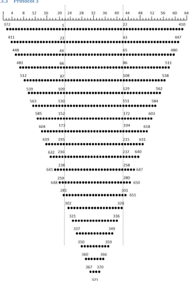
3.3.3 Protocol 3 ... 47
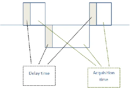
3.4 Time of measurement ... 48
4.0 Methodology ... 50
4.1 Irrigation design ... 50
7
4.3 Modified protocol comparison ... 52
4.4 Infiltration data collection and measurement procedure ... 52
4.4.1 Site selection ... 52
4.4.2 Experimental procedure ... 53
4.4.3 Variability trials ... 55
4.5 Inversion processes ... 56
5.0 Results ... 59
5.1 Protocol 2 –Homogenous profile ... 59
5.3 Protocol 3 – Homogenous profile ... 65
5.4 Protocol 2 – Variable profile ... 66
6.0 Discussion ... 75
6.1 Capability of electrical resistivity tomography to inform infiltration ... 75
6.1.1 Low resistivity layers ... 75
6.2 Informing stochastic variability ... 76
6.3 Inversion processes ... 79
6.4 Limitations of approach ... 81
6.4.1 Terrameter SAS4000 versus Terrameter LS ... 81
6.4.2 Depth based data intensity ... 81
6.5 Further work ... 82
7.0 Conclusion ... 83
7.1 Fulfilment of project aims ... 83
7.2 Application to industry ... 84
List of References ... 85
Appendix A: Project Specification ... 90
Appendix B: Experimental Design and Planning ... 91
B.1 Irrigation frame design ... 91
B.2 Risk assessment... 92
B.3 Resource requirements ... 94
B.4 Timeline ... 95
Appendix C: Experimental results ... 96
C.1 Inversion settings – homogenous profile ... 96
8
List of Figures
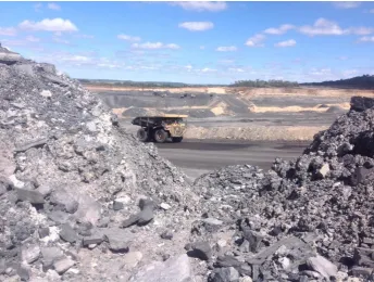
Figure 1 Example of Interburden at New Acland mine demonstrating varying shapes and sizes of coarse fragments. Interburden on the front left and front right are from two
sources, but will eventually be placed in the same soil profile. ... 13
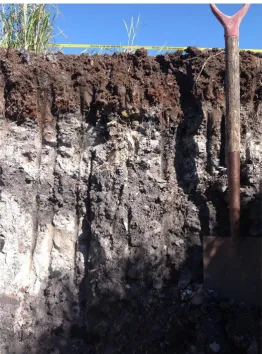
Figure 2 Soil profile of buried interburden with ≈30cm of soil as overburden. Note the heterogentiy of interburden colour (source) and coarse fragments. ... 14
Figure 3 Infiltration variability factors ... 24
Figure 4 Comparison of infiltration rates ... 25
Figure 5 Infiltration change with time ... 26
Figure 6 Flow of current from a point source with resulting potential distribution ... 33
Figure 7 Distribution from two electrodes with 1 ampere of current and resistivity of 1 𝛀.m ... 34
Figure 8 Standard electrode configuration ... 34
Figure 9 Calculation of geometric configuration constant ... 35
Figure 10 Resistivity of various soil features ... 36
Figure 11 Pseudosection for Protocol 1; axis=electrodes; data point numbers represent order of measurement. ... 45
Figure 12 Pseudosection for Protocol 2; axis=electrodes; data point numbers represent order of measurement; hashed lines represent nominal transect boundaries to define a central sequential depth. ... 46
Figure 13 Pseudosection for Protocol 3; axis=electrodes; data point numbers represent order of measurement; hashed lines represent nominal transect boundaries to define a central sequential depth. ... 47
9
Figure 15 Schematic of irrigation layout ... 51
Figure 16 Plot layout ... 52
Figure 17 2x32 cable layout (ABEM, 2012) ... 53
Figure 18 Variability trial with features exposed ... 55
Figure 19 Variability trial buried with electrodes ... 55
Figure 20 Normally inverted data set ... 57
Figure 21 Percentage change in model resistivity ... 57
Figure 22 Protocol 2 - Homogenous profile - Initial ... 59
Figure 23 Protocol 2 - Homogenous profile - 4hrs ... 59
Figure 24 Homogenous profile - hourly time-lapse percentage change ... 61
Figure 25 Change in calculated apparent resistivity (ohm m-1) after (a) 1, (b) 2, (c) 3 and (d) 4 hours of irrigation from the baseline inversion constraints (time 0) ... 64
Figure 26 Resistivity of model blocks (ohm m-1) after 4 hours of irrigation from the baseline inversion constraints (time 0) ... 65
Figure 27 Variable profile – two hour time-lapse ... 68
Figure 28 Variable profile – two hour time-lapse intervals ... 71
Figure 29 Correlation of infiltration with soil features ... 73
Figure 30 Variable profile - change in calculated apparent resistivity ... 74
Figure 31 Model blocks matching pseudo section data... 79
Figure 32 Model blocks for higher spatial resolution ... 80
Figure 33 Irrigation frame design ... 91
10
List of Tables
Table 1 Stochastic infiltration rate categories……….…78
Table A1 Personal risk rating table ... 92
Table A2 Personal hazards ... 92
Table A3 Project hazards ... 92
11
1.0 Introduction
1.1 Project overview
With the global population predicted to surpass 9.7 billion by 2050 (Nations, 2015), human reliance on the soil resource is paramount to our continued existence. In accordance with this, there is a requirement for the most efficient use of the soil system possible, so that we maximise food and energy production, without unduly degrading the soil resource. Quality of life and future development goals, globally, are contingent on this.
Critical then to this is the capacity to measure and analyse changes in a system, as well as to be able to describe/account for the complexities inherent within the system. Accurately, or at least sufficiently, monitoring changing components within the soil system provides managers’ crucial information to take corrective action across a landscape or field, ensuring environmental degradation is limited, while production requirements are optimised. Soil physical properties describe the capability of a soil to provide a physical medium for plants to take hold and thrive within, whereby production is controlled by the soil hydraulic system, which in turn, governs water (infiltration), nutrient and solute dynamics.
12 rock outcrops. Using an infiltrometer at an arbitrary point may not be representative, as a whole, of the underground pedological and geological features. To overcome this, a large number of measurements must be completed to understand the minimum and maximum (variation) and average infiltration rates of an area. This becomes a very time-consuming and laborious task over large areas. Additionally, the basic infiltrometer takes near surface measurements. Hence, depth based infiltration, and the ability to visualise this, would require significant excavation. Thus, proximal sensing methods would be of benefit.
Near surface infiltration measurement may suffice for an intensive farming situation where the soil physical properties are reasonably homogenous with area and depth; i.e. not a highly variable and complex environment. However, the accuracy and applicability of this approach for highly variable and highly complex environments decreases as the variability and complexity increases. Such environments will become increasingly common in Australia, as open cut mine sites cease production and seek to reclaim and release land for agricultural production.
13
[image:13.595.126.471.71.331.2]14
Figure 2 Soil profile of buried interburden with ≈30cm of soil as overburden. Note the heterogentiy of interburden colour (source) and coarse fragments.
With conditions for stochastic variability (e.g mine site rehabilitation) becoming more common, it is suggested that a two dimensional transect proximal imaging technique that identifies how the infiltration varies spatially should be developed. Statistically, this transect will provide a much higher chance of recognising the minimum, maximum and average infiltration rates across its length. In this case the absolute infiltration rate is of less value than understanding the level of stochastic variation. Subsequently, if the level of stochastic variation can be quantified, then the ability to account for this using a parameterised stochastic function within a soil hydraulic model (e.g. HYDRUS) is realised. HYDRUS uses a finite element mesh to model soil water dynamics within geometric parameters prescribed by the user. One of these input parameters is stochastic variability, where the expected variability parameters such as minimum, maximum, average and distribution can be randomly placed in the geometry. Hence, the ability to parametrise the stochastic variability, and account for this within HYDRUS, would effectively provide a tool to model complex and variable soil environments. Therefore, the primary issue becomes how to obtain a transect of infiltration data that parametrises the stochastic variability.
15 transect, using an ABEM Terrameter LS available from the National Centre for Engineering in Agriculture (NCEA). This technology is used extensively in geophysical studies to map rock formations or underground water (French & Binley, 2004; Greve, Acworth, & Kelly, 2008; Herman, 2001; M. Loke & Lane, 2004), which was the basis for its design. However, recent investigations have focussed on the application of this technology to soil science in the context of (Afshar, Abedi, Norouzi, & Riahi, 2015; Clément, Descloitres, Günther, Ribolzi, & Legchenko, 2009; Daily, Ramirez, LaBrecque, & Nitao, 1992; Garré et al., 2013). The ERT works as a computer with a power source and an array of electrodes, 64 for this project. In a prescribed order, the computer allocates DC current to these electrodes which transmits into the soil, where the soil features prevent some current from moving through them, dependent on their electrical conductivity. The current that is lost is measured on another prescribed electrode as a voltage drop, and through the use of Ohm’s laws, is converted into an apparent resistivity reading. Using different combinations of electrodes allows the recording of information at various depths and locations along the transect line. With a data set of apparent resistivity at a range of locations within the two dimensional transect collected, it needs to be inverted into an actual resistivity reading using the software package RES2DINV. This gives a two dimensional transect image of the electrical resistivity throughout the profile, rather than a two dimensional transect image of the apparent resistivity’s which are only relative to each other within the same soil profile. Thus, changes in soil density, inclusion of variable rock fragments, complex cumulative fragment architectures, and changes in profile moisture content should all provide different resistivity responses. Hence, the aim of this project is to determine the capability of the ERT to parameterise variable and complex soil profile stochastic infiltration along a two dimensional transect, in order to inform future infiltration modelling of such environments.
1.2 Project objectives
Based on the aim of this work, the specific objectives of the project are as follows: 1. Develop a measurement method for an infiltration scenario that can be used in
a highly variable soil environment that will at least locate the variability extremes, and potentially identify three parameters, the minimum, maximum and average infiltration rate, as well as the distribution of the infiltration variability.
2. Determine the method in which Terrameter LS measures so that the order of measurement may be manipulated to suit data analysis in a time-lapse situation. 3. Evaluate the strengths and limitations of this technology when measuring
infiltration variability.
16 protocols to collect the changing resistivity data on a fixed time-lapse. The third is data inversion and analysis so that a time lapse map of resistivity change, or infiltration will be produced.
The Terrameter is essentially a computer that assigns a direct current (DC) current through two current electrodes, and measures the voltage drop. The voltage drop is determined when the current reaches two other electrodes, in line with the current electrodes and between them, known as the potential electrodes; Ohm’s law is subsequently used to calculate the resistivity. Different combinations of these electrodes give readings at various locations on the 2 dimensional transect, both along the transect, and at various depths, with the map of which being known as a ‘pseudosection’. Four electrodes, in line and equally spaced, are required for measurement. The greater the spacing, the greater the point depth measurement. In a 64 pin line, any four pins with equidistance spacing can be used to provide a 2D depth based resistivity profile. Which electrodes are selected and in what order, is controlled by an .xml file that is supplied by the user and it is this file that can be manipulated to suit the situation required. Once the correct settings and files have been developed, a baseline type measurement is taken to identify the current state of electrical resistance in the soil, usually due to existing moisture or geographical features (ABEM, 2012). In this case, a drip irrigation line is then set up to apply water at a slow, controlled and known rate. As this occurs, the Terrameter is set to run continuously through its protocol so that as it finishes one cycle. It begins again until the soil water moves to a depth that cannot be measured, or until the soil moisture reaches an impermeable horizon, this being dependent on the environment, or until the experiment is terminated.
Resistivity 2D Inversion (RES2DINV) software will then be used to invert the apparent resistivity data into an actual resistivity data set that will determine where the soil moisture is changing at various locations throughout the profile. This enables data to be graphed in their respective time-lapsed intervals in a program such as Microsoft Excel or Matlab. The process of inversion and analysis is to be developed as part of this research project, so it will be subject to change as strengths and limitations of various methods are discovered and tested.
1.3 Assessment of consequential effects
The consequential effects of this research project can be split into two subsections, those that are contributed to by the project work itself, and those that eventuate from the resulting methodologies that will be developed.
17 There is also the requirement to dig a pit to bury rocks and create compaction to simulate a variable soil environment. The excavation site has been recommended by the landowners with the agreement that the buried material will be removed and top soil replaced at the conclusion of the project. They are aware that it will be degraded to some extent but are understanding and willing for the excavation to take place and have offered to use their own machinery to complete the operation. The excavation site is within 200m of a natural waterway and over a known underground water source so care must be taken to ensure contamination by rubbish and chemicals is minimized. The water that will be used for the infiltration tests will be taken from the bore that exists in the underground water source, without any chemical additions. This will prevent foreign liquids from entering the natural waterways.
The soil is of a coarse texture which means the placement of electrodes will likely encounter contact issues due to air gaps from the porosity within the soil, potentially reducing the effectiveness of the measurement technique. To resolve this, a mixture of water, salt, and bentonite will be used to run down the small electrode hole at each electrode to improve contact. The solution that is added to the system will not be able to be removed. However, whilst the salinity of the mixture is high, the amount for each pin is very small, meaning subsequent dilution due to rainfall will render the salinity effects as inconsequential. The landowners are aware of this and are confident that the salinity levels required for the project will not hinder plant growth.
18
2.0 Literature Review
2.1 Introduction
The past several decades have seen the human population increase at a significant rate, with the primary driver being the mechanisation of food production which has enabled more people to survive from the same arable land area. This increasing population however, has also become very energy dependent with mine sites, to some extent, competing with agriculture for use of the natural resources. As mining companies only have a certain amount of resource to extract, once a mines life has been completed, the land is usually rehabilitated to previous use, as an anthropogenic soil. Such sites, together with some other marginal agricultural soils, are renowned for being highly variable in their physical and chemical make-up leading to challenging measurement. Within the area of soil science research, some of the methods for soil data capture are relatively dated, one of which is the measurement of soil water infiltration rates, or the hydraulic conductivity of a soil. As this is a natural process, it is, like all things in nature, highly dependent on a large range of factors such as soil texture, soil structure, geological features, ion balances and compaction. This variability can often happen over quite short distances which makes measurement potentially inaccurate if the equipment is limited to a point style measurement. For this reason it is aimed that the existing technique of Electrical Resistivity Tomography (ERT) could be used to measure the change in soil water content across the length of a 2D transect of the soil profile, as opposed to a single point along that distance. Understanding the extent of the variability across this transect is very important as an input parameter for existing infiltration models. Quantifying the extremes of variability leads to more accurate outputs from existing models. With the current measurements of hydraulic conductivity, measuring the absolute minimum and maximum conductivity rates becomes labour intensive as many samples must be collected to ensure statistical confidence.
Therefore the scope of this literature review will be to identify and discuss current empirical formulas used in infiltration calculations, discuss existing 2D measurement techniques for soil moisture profiles, and discuss current uses of ERT in agriculture and identify where similar research has already been completed.
2.2 Background research in infiltration
19 1. Darcy’s Law
𝑓 = 𝐾 [ℎ0− (−𝜓 − 𝐿)
𝐿 ]
Where
𝐾 = 𝐻𝑦𝑑𝑟𝑎𝑢𝑙𝑖𝑐 𝐶𝑜𝑛𝑑𝑢𝑐𝑡𝑖𝑣𝑖𝑡𝑦 ℎ0= 𝐷𝑒𝑝𝑡ℎ 𝑜𝑓 𝑝𝑜𝑛𝑑𝑒𝑑 𝑤𝑎𝑡𝑒𝑟 𝜓 = 𝑊𝑒𝑡𝑡𝑖𝑛𝑔 𝑓𝑟𝑜𝑛𝑡 𝑠𝑜𝑖𝑙 𝑠𝑢𝑐𝑡𝑖𝑜𝑛 𝐿 = 𝐷𝑒𝑝𝑡ℎ 𝑜𝑓 𝑠𝑢𝑏𝑠𝑢𝑟𝑓𝑎𝑐𝑒 𝑔𝑟𝑜𝑢𝑛𝑑
(Mays, 2010)
Darcy’s equation above forms the basis of describing movement of water through soil. It is stating that the infiltration rate is proportional to the hydraulic gradient (Kirkham, 1972). Darcy’s law is considered a governing principle from which a range of models were derived. The earliest being Richards (1931) who uses Darcy’s law along with conservation of mass equations to develop two infiltration equations. Solving these however is challenging without the use of computer software due to the equations requiring iterative solutions (Ross, 1990). Researchers such as Ross (1990) are developing efficient models to solve these equations. Darcy’s law applies to saturated flow in a non-swelling porous media.
2. Richards Equation
𝜕𝜃 𝜕𝑡 =
𝜕
𝜕𝑧[𝐾(ℎ) ( 𝜕ℎ 𝜕𝑧− 1)]
Where
ℎ = 𝑃𝑟𝑒𝑠𝑠𝑢𝑟𝑒 ℎ𝑒𝑎𝑑 (𝑚)
𝜃 = 𝑉𝑜𝑙𝑢𝑚𝑒𝑡𝑟𝑖𝑐 𝑤𝑎𝑡𝑒𝑟 𝑐𝑜𝑛𝑡𝑒𝑛𝑡 (𝑚 3
𝑚3) 𝐾 = 𝐻𝑦𝑑𝑟𝑎𝑢𝑙𝑖𝑐 𝑐𝑜𝑛𝑑𝑢𝑐𝑡𝑖𝑣𝑖𝑡𝑦 (𝑚𝑠−1) 𝑧 = 𝐷𝑒𝑝𝑡ℎ (𝑚)(𝑝𝑜𝑠𝑖𝑡𝑖𝑣𝑒 𝑑𝑜𝑤𝑛𝑤𝑎𝑟𝑑𝑠) 𝑡 = 𝑇𝑖𝑚𝑒 (𝑠)
20 Papendick, 1984; Ross, 1990; Simunek, Huang, & Van Genuchten, 1998; Zarba, Bouloutas, & Celia, 1990; Zienkiewicz & Parekh, 1970).
3. Green-Ampt
𝐹(𝑡) = 𝐾𝑡 + 𝜓∆𝜃 ln [1 +𝐹(𝑡) 𝜓∆𝜃]
Where
𝐾 = 𝐻𝑦𝑑𝑟𝑎𝑢𝑙𝑖𝑐 𝐶𝑜𝑛𝑑𝑢𝑐𝑡𝑖𝑣𝑖𝑡𝑦 (𝑐𝑚 ℎ𝑟) 𝜓 = 𝑊𝑒𝑡𝑡𝑖𝑛𝑔 𝑓𝑟𝑜𝑛𝑡 𝑠𝑜𝑖𝑙 𝑠𝑢𝑐𝑡𝑖𝑜𝑛 (𝑐𝑚) 𝜃 = 𝑊𝑎𝑡𝑒𝑟 𝑐𝑜𝑛𝑡𝑒𝑛𝑡
𝐹 = 𝑉𝑜𝑙𝑢𝑚𝑒 𝑎𝑙𝑟𝑒𝑎𝑑𝑦 𝑖𝑛𝑓𝑖𝑙𝑡𝑟𝑎𝑡𝑒𝑑
As F is on both sides of the equation, it must be estimated initially (usually the larger solution of 𝐾𝑡 𝑜𝑟 √2𝜓∆𝜃𝐾𝑇), solved on the right hand side, then the solution used for the second iteration. This is repeated until LHS=RHS. Once the F has been found at the required time, it may be subbed into the corresponding infiltration rate equation.
𝑓(𝑡) = 𝐾 [𝜓∆𝜃 𝐹(𝑡)+ 1]
Where
𝑓(𝑡) = 𝐼𝑛𝑓𝑖𝑙𝑡𝑟𝑎𝑡𝑖𝑜𝑛 𝑟𝑎𝑡𝑒
(Mays, 2010)
The Green-Ampt model is a difficult equation to work with considering it is still an iterative solution; however it has the benefit of having definitive parameters that can all be determined experimentally, and in some instances, empirical values for the soil type can be assumed without the need for experimenting. With this, the Green-Ampt has become popular in computer modelling as the computer has the power to complete iterations in a timely manner.
21 4. Horton
𝑓𝑡 = 𝑓𝑐+ (𝑓0− 𝑓𝑐)𝑒−𝑘𝑡
Where
𝑓𝑡= 𝐼𝑛𝑓𝑖𝑙𝑡𝑟𝑎𝑡𝑖𝑜𝑛 𝑐𝑎𝑝𝑎𝑐𝑖𝑡𝑦 ( 𝑑𝑒𝑝𝑡ℎ
𝑡𝑖𝑚𝑒) 𝑎𝑡 𝑡𝑖𝑚𝑒 𝑡 𝑓𝑐= 𝐼𝑛𝑓𝑖𝑙𝑡𝑟𝑎𝑡𝑖𝑜𝑛 𝑟𝑎𝑡𝑒 𝑜𝑓 𝑠𝑎𝑡𝑢𝑟𝑎𝑡𝑒𝑑 𝑠𝑜𝑖𝑙 𝑓0= 𝐼𝑛𝑓𝑖𝑙𝑡𝑟𝑎𝑡𝑖𝑜𝑛 𝑟𝑎𝑡𝑒 𝑜𝑓 𝑢𝑛𝑠𝑎𝑡𝑢𝑟𝑎𝑡𝑒𝑑 𝑠𝑜𝑖𝑙 𝑘 = 𝐷𝑒𝑐𝑎𝑦 𝑐𝑜𝑛𝑠𝑡𝑎𝑛𝑡 𝑠𝑝𝑒𝑐𝑖𝑓𝑖𝑐 𝑡𝑜 𝑡ℎ𝑒 𝑠𝑜𝑖𝑙
(Horton, 1941)
Horton’s model can also be modified to suit a volumetric measurement rather than the infiltration rate that is shown above.
Horton’s model is the most common selection for most hydrologists since it incorporates a saturated or steady state infiltration rate which is different to the initial or unsaturated rate. Zhenghui et al. (2003) notes that this difference is due to factors influencing the properties of the surface soil and how the initial moisture is adsorbed, rather than the preferential or matric flow that occurs at depth. The advantage of using Horton over Kostiakov, is that there is an initial finite condition, 𝑓0 (Hillel, 1980). The limitation of the Horton model is the time consuming application of using field-gathered measurements as the constants in the empirical equation (Hillel, 1980). The Horton model itself is a simplification of the Richards equation where the soil water diffusivity (D) and the hydraulic conductivity (K) are assumed not to be a function of the soil moisture, when in fact they are. However by making this assumption, the Horton equation becomes solvable making it simple to use.
5. Kostiakov
𝑓(𝑡) = 𝑎𝑘𝑡𝑎−1
Where ‘a’ and ‘k’ are empirical values. (Kostiakov, 1932)
Much like Horton’s model, integrating Kostiakov’s equation will give a volumetric solution, rather than an instantaneous rate.
22 The Kostiakov equation is an empirical equation that was the best curve fit available from measured field data (Turner, 2006). Fox, Phelan, and Criddle (1956) developed a type of test function that allowed the values of ‘a’ and ‘k’ to be determined. In addition, their function presented as a linear solution if the Kostiakov equation could be applied, and nonlinear if it were an incorrect fit (Naeth, Chanasyk, & Bailey, 1991).
The Kostiakov equation was found to be more accurate than the Philip model for irrigated fields where the spatial variability in the infiltration data was larger (Ghosh, 1980), but less accurate for semi-arid rangelands, typically those found throughout the United States and Australia (Gifford, 1976). This finding led Gifford (1976) to believe that the constants used in the Kostiakov equation were more comparable to vegetation indices rather than factors influencing the soil conditions.
6. Philip
𝑓(𝑡) =𝑆 2𝑡
−1 2+ 𝐶𝑎
Where
𝑆 = 𝑆𝑜𝑟𝑝𝑡𝑖𝑣𝑖𝑡𝑦 𝐶𝑎= 𝐶𝑜𝑛𝑠𝑡𝑎𝑛𝑡
(Philip, 1957)
The 𝐶𝑎 constant is a value dependant on the initial water content, and the application rate (Turner, 2006).
The Philip model was developed as a solution to the Richards equations that used Darcy’s law as a fundamental (Turner, 2006). The solution is provided for horizontal and vertical infiltration under a range of conditions. It can be seen that although different methods have been taken, the Philip model is quite similar to the Kostiakov equation previously discussed. Youngs (1968) developed a number of solutions to estimate accurately, the sorptivity factor and the 𝐶𝑎 term. The methodology followed for this estimation is beyond the scope of this literature review. The Philip equation is limited to a homogenous soil under ponded conditions with uniform initial moisture content, and is subsequently limited much like the Green-Ampt model, but without the need for an iterative solution.
7. Holtan
𝑓𝑝= 𝐺𝐼𝑎𝑆𝐴1.4+ 𝑓𝑐
Where
𝑆𝐴 = 𝐴𝑣𝑎𝑖𝑙𝑎𝑏𝑙𝑒 𝑠𝑡𝑜𝑟𝑎𝑔𝑒 𝑖𝑛 𝐴 ℎ𝑜𝑟𝑖𝑧𝑜𝑛
23 SA is calculated as:
𝑆𝐴 = (𝜃𝑠− 𝜃𝑖)𝑑 Where
𝜃𝑠= 𝑆𝑎𝑡𝑢𝑟𝑎𝑡𝑒𝑑 𝑤𝑎𝑡𝑒𝑟 𝑐𝑜𝑛𝑡𝑒𝑛𝑡 𝑜𝑓 𝑡ℎ𝑒 𝑠𝑜𝑖𝑙 𝜃𝑖= 𝐴𝑐𝑡𝑢𝑎𝑙 𝑣𝑜𝑙𝑢𝑚𝑒𝑡𝑟𝑖𝑐 𝑤𝑎𝑡𝑒𝑟 𝑐𝑜𝑛𝑡𝑒𝑛𝑡 𝑑 = 𝐷𝑒𝑝𝑡ℎ 𝑜𝑓 𝐴 ℎ𝑜𝑟𝑖𝑧𝑜𝑛
(Holtan, 1971)
The Holtan model is based on empirical values that are readily available to the public, regarding a whole range of soil types commonly farmed for agriculture (Turner, 2006). It is based on the concept that the governing factors in the infiltration rates are the current volume of water in the soil, the volume of water at saturation, and other influences in the A horizon such as root activity and preferential flow paths (Rawls, Ahuja, Brakensiek, & Shirmohammadi, 1993).
There are comprehensive tables available for substitution of variables into the initial Holtan equation; however the challenge occurs when deciding what depth to calculate SA to as this becomes quite subjective (Ortiz-Reyes, 1979). It is also noted that the Holtan equation makes no reference to time, as it makes the infiltration rate a function of water storage (Turner, 2006). There are methods making reference to time but they include solving another water storage equation simultaneously and this is out of the scope of this review.
All these methods have their strengths and weaknesses, the challenge lies in selecting the correct equations for the situation at hand. The scope of this project is to locate and quantify infiltration variability, not to develop an infiltration model as these are already in abundance, and widely accepted as being adequately developed. It is intended that an accurate understanding of the infiltration variability will provide the means for an increased level of accuracy within existing models.
2.3 Variable infiltration environments
24
2.3.1 Causes of variability
Consider the following Figure 3.
Figure 3 Infiltration variability factors
Under the free soil condition, the infiltration rate will be purely dependent on the texture, organic matter, initial moisture content, and porosity (Morin & Benyamini, 1977). Under the compaction condition, the infiltration rate will be dependent on the same factors, but lower due to a reduction in soil porosity. And under the rock condition, the infiltration rate will be limited to the permeability of the rock, which is dependent on the extent of fracturing and the resulting pore network.
Brouwer, Prins, Kay, and Heibloem (1988) identify common soil infiltration rates as follows:
- Clay 1-5 mm hr-1
- Clay loam 5-10 mm hr-1 - Loam 10-20 mm hr-1 - Sandy Loam 20-30 mm hr-1 - Sand < 30 mm hr-1
These values are derived from a saturated flow experiment on soils that were not cultivated, conducted by researchers from the Food and Agriculture Organisation (FAO). They were not collected from various data sets around the world, however they were measured on soils that were classed according to the Soil Map of the World produced by the FAO and United Nations Educational, Scientific and Cultural Organisation (UNESCO), which is quite similar to the USDA Soil Taxonomy. Although the infiltration rate is highly dependent on a range of factors, the above rates give a reasonable ball park figure. They are suitable for the purpose of comparison with compaction and rock features.
Douglas and Crawford (1993) found that under a severe trafficking situation in a sandy loam grassland system, infiltration was reduced by as much as 76%, with recorded values of 26.9 mm hr-1 down to 6.3 mm hr-1 due to a reduction in the macro pore volume. Ryan, Monroe, Kacemi, and Monem (1990) found that under compacted clay, soil infiltration was reduced by 60% in the 0-15cm range, 80% in the 15-30cm range, and 55% in the 30-205cm range, all to values less than 2 mm hr-1, with 0.5 mm hr-1 at depth using a ‘conventional’ tractor.
Rock
Compaction
25 Caputo and Carlo (2011) examined infiltration rates on a hard sedimentary, fractured limestone rock and a soft sedimentary rock, calcarenite. They report that under laboratory conditions where preferential flow paths such as cracks and fissures are excluded, the limestone had an infiltration rate of 0.875 mm hr-1 which they attribute to the rock porosity. The calcarenite was found to have an infiltration rate of 20 mm hr-1 however they note that cracks and fissures were not excluded due to the aggregate arrangement being crumbly with large preferential flow paths networked throughout the sample.
These three different situations are represented graphically to demonstrate their comparison in Figure 3.
Figure 4 Comparison of infiltration rates
Although the above graph is a collection of various datasets in different locations collected for different research purposes, the point it makes is that as soon as rock and compaction are introduced, the infiltration rate of that profile becomes highly varied. Understanding where these disruptions occur and in what area of the profile is important when quantifying the average infiltration rate and the variability parameters as they will be highly influenced by these features.
Assume a 2D transect of 10m, with a random distribution of compaction and rock features throughout it. Taking a series of infiltration measurements with a traditional ring infiltrometer from the surface will require a very narrow spacing to ensure accuracy. However this becomes problematic as the water introduced to the system from each test may influence the adjacent sites if for instance, the water meets a rock and begins to flow laterally around the surface. If that spacing is widened to avoid this scenario, there is a likely chance that features will be missed. Statistically this is a very complicated situation as there may be a reading of 30 mm hr-1, followed immediately by a 0.5 mm hr-1 measurement. This makes curve fitting very difficult as there will be large error bars and inaccurate averages associated with the infiltration rates.
0 5 10 15 20 25 30 35
Free Soil Compaction Rock
In
fi
ltr
ation
R
ate
(
m
m
/h
r)
Comparison of infiltration rates
Sand
Clay
26
2.3.2 Unsaturated and saturated flow
The infiltration rate that is officially recorded from an experiment is very important as it is dependent on the soil properties, and as the soil moisture content increases throughout the trial, the properties will change from unsaturated to saturated. Such change directly affects the infiltration rate as reviewed in the previous models and equations.
In saturated flow, both the micro and macro pores are filled with water and transmission through the profile is driven by large differences in pressure and gravity (Singer & Munns, 2006). Movement in a coarse-grained soil under this condition can be quite fast if there is no stratification between horizons and there is a ponded head on the surface. When the soil is unsaturated, the macro pores have been emptied by gravity and the surface area of the pore network becomes the critical factor with respect to how much water is retained and the ease of its movement (Oades, 1984). The water that remains becomes tightly held in thin films around the interior surface of the pore network. This hinders soil water movement considerably as hydraulic friction is increased as the width of the water film is decreased (Singer & Munns, 2006). This means that movement is no longer driven singularly by gravity, but by a potential gradient (𝜓) consisting of gravity (𝜓𝑔), pressure (𝜓𝑝), matric potential (𝜓𝑚), and solute (osmotic influence) (𝜓𝑠) (Singer & Munns, 2006). The addition of a matric and solute potential create a higher infiltration rate than under a saturated situation.
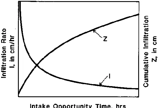
The change from being driven by gravity and pressure, to a potential gradient occurs over a different time period for all soils. However the trends are the same. Consider Figure 55. As the cumulative infiltration increases, which is equal to the soil moisture, the infiltration rate decreases as the matric and solute potentials are equilibrated and gravity and pressure become the driving factors. As the infiltration rate decreases, it approaches an asymptote that is termed the “basic infiltration rate” (Walker, 1989).
[image:26.595.105.384.507.697.2](Walker, 1989)
27
2.4 2D Measurement of soil moisture profiles
Soil moisture measurement can be performed through a variety of methods. These methods are generally classified into three categories, the direct measurement, indirect measurement, and soil water potential measurement (Organization, 2014). Each of these have their own limitations and benefits which creates a framework of questions that allows the correct measurement technique to be selected based on the requirements and limitations of the specific project. For instance, broad scale measurement, site specific measurement or destructive measurement methods all contribute to the preferred measurement technique chosen. These measurement techniques are broken into three categories and consist of the following (Organization, 2014).
1) It is determined whether the measurement needs to quantify soil water or soil water potential. Gravimetric soil water is important for compaction type projects such as machinery in agriculture or civil construction sites, but soil water potential is important to agronomy in agriculture due to the plants physically creating a negative pressure in order to suck water from the soil. Water in the soil is not available to plants if the suction required is beyond the wilting point of the plant.
2) Direct vs indirect methods. Direct measurement is destructive as the sample needs to be removed from the environment and taken to a laboratory. Thus, if a broad scale understanding is required from this method, there is a need for a large area of representative soil that can provide a multitude of samples to achieve an accurate result. This involves a lot of labour and is destructive to the environment. The alternative is an indirect measurement where equipment is placed in the soil to measure a soil property that is known to strongly influence the moisture status, such as conductivity.
3) Understanding the applicability of each method in terms of the regional resources such as labour to undertake sampling, the quality of the equipment available such as a laboratory or measurement instruments, and the knowledge base of the people involved when using advanced equipment or undertaking data processing.
2.4.1 Direct measurement and interpolation
Direct measurement refers to the physical removal of a sample from the soil environment and quantifying water content as gravimetric moisture content and involves large amounts of time, labour, and is destructive to the test site. Currently, oven drying is the only truly direct measurement of the gravimetric moisture content.
Oven drying
28 a certain amount of time (Australia, 1990). Once the standard has been followed, there is a formula to be completed to calculate the moisture content as a percentage of the soil’s dry weight.
𝑀𝐶% = (𝑊2− 𝑊3 𝑊3− 𝑊1
) ∗ 100
Where
𝑊1= 𝑊𝑒𝑖𝑔ℎ𝑡 𝑜𝑓 𝑡𝑖𝑛 (𝑔)
𝑊2= 𝑊𝑒𝑖𝑔ℎ𝑡 𝑜𝑓 𝑚𝑜𝑖𝑠𝑡 𝑠𝑜𝑖𝑙 + 𝑡𝑖𝑛 (𝑔) 𝑊3= 𝑊𝑒𝑖𝑔ℎ𝑡 𝑜𝑓 𝑑𝑟𝑖𝑒𝑑 𝑠𝑜𝑖𝑙 + 𝑡𝑖𝑛 (𝑔)
This method is limited to obtaining a spatial point measurement of the soil moisture, so when measuring the variation over a 2D transect, regular samples need to be taken and the values between them interpolated. This is a very time consuming method as drying takes approximately three days and samples have to be weighed before and after drying. Although each measurement is accurate, in a highly variable soil the statistical chances of collecting data on each end of the variability spectrum is so slight that there is no literature identifying how many samples are required to confidently understand the variation in different soil conditions. Wang, Engman, and Ungar (2010) used oven dried samples at 50m spacings for a long transect as a ground proofing technique to test airborne moisture instruments and noted that no quantitative assessment was made when investigating the variability parameters.
This inability to quantify the variability parameters makes creating a 2D transect of infiltration over any distance, an inefficient and expensive operation when using the oven drying method.
2.4.2 Indirect measurement techniques
Indirect measurement techniques enable repeated measurements of a sample without disturbing the soil for each sample thus the soil is left in the environment and monitored as the volumetric moisture content, independent of the soil physical properties such as soil density (Organization, 2014).
Soil water dielectrics
29 Capacitance probes measure the dielectric constant of a soil by creating an oscillating electrical field between two rings within a tube. This field extends through the wall of the capacitor, usually made of PVC, and into the soil medium. The frequency of this oscillation changes with the moisture in the soil medium and this is what is monitored and related back to the dielectric constant, and subsequently the volumetric soil moisture (Dirksen, 1999). Capacitance probes are widely used and regarded as an accurate means of determining soil moisture given that they are calibrated correctly. T. J. Jackson (1990) notes that the most consistent and accurate method of calibrating a capacitance probe is using it in a liquid of known dielectric properties. This method will give results with less variability than most dielectric models will predict.
Time-domain reflectometry is quite similar to a capacitance probe; however instead of measuring the change in the oscillation frequency, it measures the magnitude of a return pulse from the end of a transmission line. This electromagnetic pulse is generated by a pair of parallel rods that push it along a transmission line into the soil, part of which is adsorbed, and part reflected. In the soil, the return wave is due to a step decrease meaning the reflection has the opposite signal to the generated wave (Hoekstra & Delaney, 1974; Topp, Davis, & Annan, 1980). The intensity of this return wave can be measured and related to volumetric soil moisture.
Radiological methods
Radiological measurements of soil water occur via two methods. The first and most commonly used involves quantifying and understanding how high energy neutrons interact with hydrogen atoms in the soil, generally being in the soil water. The second is usually reserved for laboratory measurement due to gamma radiation being more dangerous to work with and involves quantifying the attenuation of a gamma wave as it moves through the soil environment.
30 Nicolls (1981) found that incorrect calibration of a specific test site generated errors from soil hydrogen influence to affect results by up to 40%. They note that other minerals exist that have tendencies to absorb neutrons such as Boron and Iron, however they conclude that while calibration is difficult, when done correctly, neutron scattering techniques are a reliable and repeatable method of soil water measurement.
Gamma wave attenuation techniques have largely been reserved for laboratory measurements since dielectric techniques became available for field use. The method of gamma-ray attenuation involves propagating a gamma wave along a thin layer of soil approximately 25cm under the surface. The scattering and absorption of these waves is driven by the density of the medium the wave encounters, so assuming the dry density of the medium remains unchanged, the change in density will come from a change in water content. This provides the grounds for measuring the soil moisture as a function of a change in saturated density (Susha Lekshmi, Singh, & Shojaei Baghini, 2014). The limitation of this technique in a field situation arises when the dry density changes, which can be influenced by plant roots pushing into the top 25cm, as well as compaction from machinery or livestock on the surface.
Soil water potential
Measuring the soil water potential is done with three different instruments, tensiometers, resistance blocks and psychrometers. These are all similar in that they use a porous material to measure a negative pressure.
Tensiometers consist of a small ceramic cup on the end of a sealed plastic tube. When saturated and placed in the soil, the water will move from the ceramic into the soil matrix to achieve equilibrium. This water movement from the ceramic outwards creates a negative pressure through the plastic tube which is registered on a recording instrument at the top (Marthaler, Vogelsanger, Richard, & Wierenga, 1983).
Resistance blocks consist of a small block of porous material where two electrodes are placed a known distance apart. As the soil water moves into the ceramic block to reach equilibrium, the electrodes measure the resistance between them. As they are dependent on an electrical current, salinity will influence results and must be taken into account (Werner, 1995).
Psychrometers are primarily used for laboratory measurements and require extensive calibration when used in the field. They work via a thermocouple inside a porous chamber that is cooled to condense water. As this water is then evaporated there is a change in temperature and a current is produced along a wire which is measured by a meter (Merrill & Rawlins, 1972).
2.4.3 Other geophysical techniques
31 adopted across a broad range of industries such as agriculture and mining, and government compliance agencies.
Ground penetrating radar
Ground penetrating radar (GPR) uses electromagnetic waves at frequencies between 50MHz and 1200MHz, depending on the depth required (Lunt, Hubbard, & Rubin, 2005). The mechanism consists of a transmitter and a receiver which propagates a wave at the desired frequency between the pair. The wave splits into three sections, the airwave that travels directly to the receiver, the ground wave which travels at the ground surface, and a reflection wave that travels through the soil to a certain depth and is reflected to the receiver. This reflection wave is manipulated by subsurface contrasts, with the primary contrast usually being soil moisture, unless there are major geological features buried within the reflection depth (Powers, 1997). Chan and Knight (1999); Martinez and Byrnes (2001); Van Dam and Schlager (2000) all showed that the driver of the reflection variation in a shallow surface, commonly at depths associated with agriculture, was volumetric water content because soil texture changes were not able to produce such large contrasts, and water was the only material in the soil environment that had a high enough dielectric constant to create the manipulation in the reflection wave. Huisman, Sperl, Bouten, and Verstraten (2001) found that existing calibration equations such as Topp’s equation that are used for calibrating time domain reflectometry equipment can be directly used to calibrate GPR data. The only limitation that Huisman, Snepvangers, Bouten, and Heuvelink (2002) found when mapping spatial variation was that heavier textured soil increased the inaccuracy of the volumetric moisture reading, and this was to be expected due to the conductivity of clay particles. GPR has been proven to be an efficient method of collecting soil moisture data for larger areas as the resolution of large scale changes is captured and represented well on the variogram of the data when compared to time domain reflectometry (Huisman et al., 2002). This is due to time domain reflectometry being overly sensitive to changes in soil properties such as compaction, while GPR averages such influences over a larger area. This suggests that one technique is not better than the other, but that each are suited to different situations.
Microwave and thermal infrared
32
Electromagnetic induction
Electromagnetic induction (EM) techniques have been used for the last 30 years when identifying the spatial variability of soil moisture. EM measures the bulk conductivity of a soil by transmitting a magnetic field from one end of the device, and sensing the return field through a receiver coil. Depending on how far these coils are apart, the magnetic field will reach to a specific depth. The magnetic field that is induced produces ‘eddy currents’ throughout the soil profile to the known depth and induces a magnetic field within the soil. The strength of this secondary field is measured by the receiver and is dependent on the bulk conductivity of the soil to the nominated depth (Schneider, 2016). Kachanoski, Wesenbeeck, and Gregorich (1988) showed that the bulk electrical conductivity read by EM methods was responsible for 96% of the spatial variability in the soil moisture when ground proofed over locations with a range of volumetric soil moisture readings, and a range of different textures.
2.4.4 ERT as used in geophysical applications
ERT is used within the industry of geophysics through the direct current resistivity application to mapping subsurface geological features, locating groundwater sources and monitoring ground water pollution. ERT is used in engineering to locate subsurface features such as mineshafts, cavities, geological fault lines, underground permafrost, etc. and in archaeology to map buried ancient buildings (J. M. Reynolds, 2011). This resistivity method is based on Ohm’s laws. An electrical current I (ampere) is passed through a medium of length L (metres). The material has a resistance R (ohm) which causes a voltage drop V (volt) across this length, presuming the material is homogenous within this range (L) (Caputo & Carlo, 2011). Ohm’s first law in the form of a vector for current flow through a continuous media is given a:
𝐽 = 𝜎𝐸 (1)
Where 𝐽 = 𝐶𝑢𝑟𝑟𝑒𝑛𝑡 𝐷𝑒𝑛𝑠𝑖𝑡𝑦
𝜎 = 𝑚𝑒𝑑𝑖𝑎 𝑐𝑜𝑛𝑑𝑢𝑐𝑡𝑖𝑣𝑖𝑡𝑦
𝐸 = 𝐸𝑙𝑒𝑐𝑡𝑟𝑖𝑐 𝑓𝑖𝑒𝑙𝑑 𝑖𝑛𝑡𝑒𝑛𝑠𝑖𝑡𝑦
M. Loke and Lane (2004) note that more commonly, the medium resistivity is used and is the reciprocal of 𝜎, meaning (𝜌 =1
𝜎). The electrical field intensity (E) is not useful, however the electric field potential is, and the pair are related in equation (2).
𝐸 = −∇Φ (2)
It can be noted that the flux has been introduced with equation (2) which is a measure of the electrical flow through a unit area.
Combining these equations creates an equation for the current density (the flow of charge per time, over a cross sectional area), which is dependent on the conductivity and the flux over a given field.
33 In most resistivity surveys, the current originates from an electrode in the ground which is a point source located at (𝑥𝑠, 𝑦𝑠, 𝑧𝑠) that influences an elemental volume (Δ𝑉). Dey and Morrison (1979) investigated a numerical solution to solving 3D potential distributions around a point source of current and introduced the empirical function, the Dirac delta function (𝛿) in order to remove dimensions from the current density to form a relationship with current itself. This leads to the equation (4)
∇. 𝐽 = (Δ𝑉𝐼) 𝛿(𝑥 − 𝑥𝑠)𝛿(𝑦 − 𝑦𝑠)𝛿(𝑧 − 𝑧𝑠) (4) When equations (4) and (3) are combined, the following is produced.
−∇ ∙ [σ(x, y, z)∇Φ(x, y, z)] = (𝐼
Δ𝑉) 𝛿(𝑥 − 𝑥𝑠)𝛿(𝑦 − 𝑦𝑠)𝛿(𝑧 − 𝑧𝑠) (5) This is the equation that provides a graphical solution to the potential distribution in the ground resulting from a point current source (M. Loke & Lane, 2004). The numerical solution to this equation comes in the form of forward modelling equations that have been developed for a variety of different cases by different researchers.
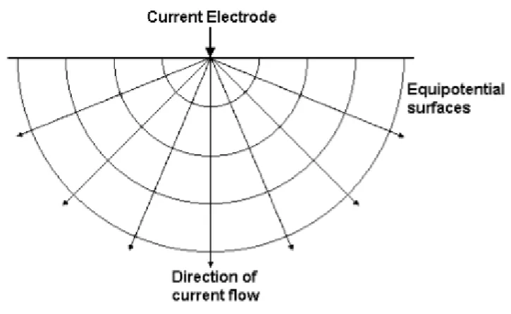
Equation (5) is a complicated equation but can be graphically displayed for ease of understanding in Figure 6.
[image:33.595.117.480.377.600.2](M. Loke & Lane, 2004)
Figure 6 Flow of current from a point source with resulting potential distribution
34 (M. Loke & Lane, 2004)
Figure 7 Distribution from two electrodes with 1 ampere of current and resistivity of 1
𝛀.m
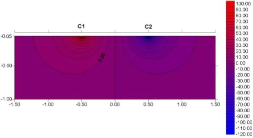
[image:34.595.100.514.72.298.2]The numerical solution of equation (5) models how the potential is distributed out from a point source. In most surveys, the standard electrode configuration is two current electrodes (C1 and C2) that induce the current, and two potential electrodes (P1 and P2) that measure the voltage drop. They are arranged as displayed, Figure 8.
Figure 8 Standard electrode configuration
As equation (5) models the potential distribution, the potential at a specific point is found by manipulating the width between the electrodes. The wider they are, the deeper the resulting potential will be from the surface. When using a four electrode array, the calculation for the potential difference is as follows
ΔΦ = 𝜌𝐼 2𝜋(
1 𝑟𝐶1𝑃1
− 1
𝑟𝐶2𝑃1 − 1
𝑟𝐶1𝑃2 + 1
𝑟𝐶2𝑃2
) (6)
Where
ΔΦ = 𝑃𝑜𝑡𝑒𝑛𝑡𝑖𝑎𝑙 𝐷𝑖𝑓𝑓𝑒𝑟𝑒𝑛𝑐𝑒 𝜌 = 𝑀𝑒𝑑𝑖𝑢𝑚 𝑅𝑒𝑠𝑖𝑠𝑡𝑖𝑣𝑖𝑡𝑦
35 The limitation of equation (6) is that the potential difference found is on the assumption of a homogenous medium (M. Loke & Lane, 2004). As the majority of situations will undoubtedly be heterogeneous, the equation is changed to calculate the apparent resistivity.
𝜌𝑎= 𝑘 ( ΔΦ
𝐼 ) (7)
Where
𝑘 = 2𝜋 (𝑟1
𝐶1𝑃1− 1 𝑟𝐶2𝑃1−
1 𝑟𝐶1𝑃2+
1 𝑟𝐶2𝑃2)
k is the geometric configuration of the electrodes so it only needs to be calculated once for each trial, hence the allocation of it to a constant. k can also be calculated from a simpler approach for a given protocol. In this project, the Wenner protocol is used.
(M. Loke & Lane, 2004)
Figure 9 Calculation of geometric configuration constant
The Terrameter itself measures an apparent resistance value R which according to Ohm’s law, is equal to ΔΦ𝐼 as seen in equation (7). This means that in a real world application, the more difference there is in electric potential, such as a rock compared to water, the more apparent resistivity the machine will measure. This measurement occurs over the 651 electrode combinations available, to produce a pseudosection of the apparent resistivity when compared with other points in the same soil profile. A specific reading does not necessarily mean a certain soil characteristic, i.e a reading of 10 ohm.m does not always mean dry sand, there are a range of factors that influence that apparent resistivity reading. This is where calibration and data inversion become important to ensure the recorded data is converted into an actual resistivity measurement that is representative of the soil conditions in the sample. Without these processes, the apparent resistivity reading is not useful for any type of interpretation or analysis.
36 a baseline measurement for apparent resistivity, and any changes from this baseline measurement at depth represent a change in soil moisture.
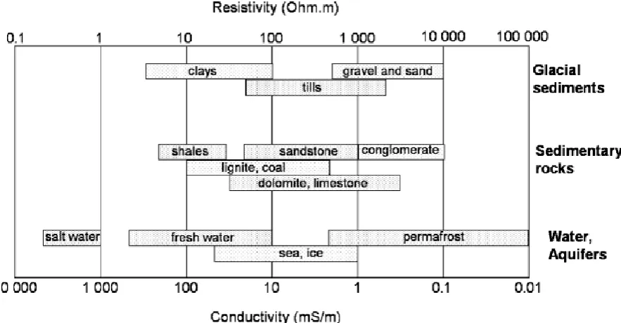
[image:36.595.104.546.223.453.2]For different experimental locations, the baseline apparent resistivity will not be the same, as it is unlikely that a second soil profile will have identical features to the first. The apparent resistivity for rock, sand and clay, compacted and uncompacted, and water all differs, depending on the features of the specific sample. Some example ranges of apparent resistivity have been identified by (Samouëlian, Cousin, Tabbagh, Bruand, & Richard, 2005) in Figure 10, and lie on a logarithmic scale.
Figure 10 Resistivity of various soil features
2.4.5 Summation and discussion of all methods
Geophysical techniques as a whole can be classed into two main categories: those that measure subsurface responses to artificially-induced electrical, seismic and electromagnetic signals, referred to as active measurement techniques; and passive techniques that measure the earth’s natural magnetic, electrical and gravitational fields (Caputo & Carlo, 2011). In this way, it is much the same concept as the comparison of direct and indirect measurement techniques that have previously been discussed. Oven drying cannot be used to monitor soil moisture change over time as each point requires soil removal and this destruction means anything more than instantaneous soil moisture is impossible. However the use of oven drying soil samples is important in order to establish a baseline measurement for initial soil moisture across a transect, and down to depth. In this regard, the use of oven drying is useful when used in conjunction with the other infiltration measurement techniques. Within this project, it is used for calibrating the Terrameter in accordance with the initial moisture conditions.
37 alternative, however these measure volumetric moisture content as they are actually reading the electrical properties of the soil. In order to convert this back to a gravimetric reading for direct comparison with oven drying, the bulk density of the soil must be known. The use of a capacitance probe is most prevalent in agricultural irrigation systems where the user will place it in the soil, take some bulk density readings for calibration, and leave it for the entire season to record on a fixed time interval. This allows relatively real time moisture readings which are vital for irrigation scheduling. Currently, there is interest in using remote sensing techniques for broad scale soil moisture measurement which could potentially limit the use of a capacitance probe moving forward, however for the time being, the capacitance probe will likely remain the measurement technique of choice in agriculture due to its proven historical performance. In other applications, the limitations of both frequency and time-domain reflectometry exist when used in dry cracking clay where there are air gaps immediately around the sensor, or in stony or shaly soil profiles. Any soil feature that will change the electrical properties will cause the probe to become unreliable.
The alternative to the probe for long term soil moisture is the use of satellite or other remote sensing instruments, and appropriate hydrologic models. The combination of the sensor and model is critical, since each technique can be inaccurate (Fang et al., 2016). Systems such as ASMR-E, RFID, SAR, and many others have been developed in the past decade to facilitate the large scale measurement of soil moisture. The development has been driven by researchers from a large array of fields, all with their own ambitions for the technology, making the progression of sensor and model systems a very interesting and rapidly advancing area of development. One area of this advancing research is in-situ based sensors, such as ERT.
2.5 2D measurement of soil infiltration using ERT
The method of ERT lends itself to a repeatable measurement on the same location as the electrodes are fixed. This enables the ERT to be run and re-run in successive events throughout a single day, as each measurement sequence takes a fixed amount of time (93min for the settings discussed in Chapter 3). If there is the ability to measure the same set of 651 points repeatedly, then changes at each of these points can be monitored through a time-lapse sequence. The changes at each point can be quantified as anomalies through the following equation;
∆𝜌𝑡= 𝜌𝑡−𝜌0
𝜌0
𝑊ℎ𝑒𝑟𝑒 𝜌0= 𝑖𝑛𝑖𝑡𝑖𝑎𝑙 𝑟𝑒𝑠𝑖𝑠𝑡𝑖𝑣𝑖𝑡𝑦 𝑟𝑒𝑎𝑑𝑖𝑛𝑔
38 horizontal) of each measurement is known for distance measurement, then the rate at which the resistivity variation moves downwards, can be correlated to the rate at which the wetting front moves through the profile. This concept provides the grounds for infiltration rate measurement, which can be interpreted into a number of methods, ultimately coming to the quantification of the hydraulic conductivity.
The use of ERT in temporal measurement has been done in a number of studies (Cassiani, Bruno, Villa, Fusi, & Binley, 2006; French & Binley, 2004; P. Jackson et al., 2002; Slater et al., 2002), in a range of conditions with different experimental outcomes. The difference of this project is the time-lapse is occurring over a number of hours, rather than months as was seen in the literature.
2.6 Limitations of ERT
ERT provides very useful information in regards to the features of a soil profile, however if the interpretation or collection of the information is not correct, then the data becomes misleading. There are a number of limitations that exist with this technology that must be considered when taking measurements and inverting data.
a) Poor electrode ground contact
Soil/electrode contact is crucial when attempting to put current into the soil. If the computer is putting a fixed amount of current into the electrode and it cannot transfer the prescribed amount to the soil, due to the soil being stony, shaly, or dry, then there will be an incorrect reading of the voltage drop into the potential electrode. This is overcome by placing a salt and bentonite mixture with the electrode to increase the transferability of current.
b) Poor current penetration
If there is a high resistivity layer in the top part of the profile, then the current will have difficulty penetrating through to the lower part of the profile. This happens in reverse as well, with a low resistivity top layer, the current can become trapped and not be accurate in the lower layer. There is no solution for this. When there is a highly contrasting layer in the data consideration of said limitation should be applied. This contrast can also happen when there is a gravelly surface, with a clay or saline subsoil, for example.
c) Not letting current charge decay
39 d) Limited by laws of physics
40
3.0 Terrameter Function and Protocol Development
As suggested earlier, the Terrameter is, in its most basic form, a computer that allocates current to selected electrodes known as current electrodes, and records the resistance that is created by the soil medium through other electrodes known as potential electrodes. With this in mind, it is important to have a thorough understanding of how it works to ensure there are no incorrect assumptions when analysing the data. Therefore, this chapter will first report on how the Terrameter actually works, what each of the settings control, and detail how the Terrameter performs a measurement. Then using this knowledge, a new set of protocols will be coded for the specific application of infiltration measurement in order to maximise the potential that ERT brings to soil water dynamics. These new protocols will be designed with ERT limitations in mind as to minimise the potential errors that were documented in the previous section. It is also intended that they will be universally compatible with other ERT platforms, not just the brand that is used for this project.
This chapter is crucial to developing appropriate strategies for using ERT in this application, and should not be confused as methodology; it is original work. ERT is not specifically designed to monitor short interval time-lapse, so a thorough understanding of how it can be manipulated to do this, is important. It is also important that a document be developed so if the work is to be repeated, the user ca