1stPan-American Congress on Computational Mechanics - PANACM 2015 XI Argentine Congress on Computational Mechanics - MECOM 2015 S. Idelsohn, V. Sonzogni, A. Coutinho, M. Cruchaga, A. Lew & M. Cerrolaza (Eds)
USING 1D-IRBFN METHOD FOR SOLVING A HIGH-ORDER
NONLINEAR DIFFERENTIAL EQUATION ARISING IN MODELS OF
ACTIVE-DISSIPATIVE SYSTEMS
DMITRY V. STRUNIN1, DUC NGO-CONG2AND RAJEEV BHANOT3
1Computational Engineering and Science Research Centre and Faculty of Health, Engineering and Sciences
University of Southern Queensland Toowoomba, QLD 4350, Australia
2Computational Engineering and Science Research Centre University of Southern Queensland
Toowoomba, QLD 4350, Australia [email protected]
3Computational Engineering and Science Research Centre and Faculty of Health, Engineering and Sciences
University of Southern Queensland Toowoomba, QLD 4350, Australia
Key words:1D-IRBFN Numerical Method, Nonlinear Active-Dissipative PDE
1 INTRODUCTION
The following model presents a single-equation simulation tool for certain type of active systems with dissipation,
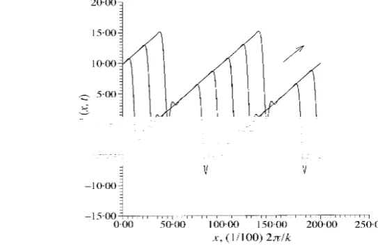
[image:2.595.231.503.357.534.2]∂tu= −A(∂xu)2∂2xu+B(∂xu)4+C∂6xu , (1) A, B, C > 0. In particular, Eq. (1) simulates combustion waves (fronts) having the shape of one or more steps [1] and developing instabilities in nonlocal reaction-diffusion systems [2]. In the context of combustion waves,ustands for the distance, measured along, say, axisz, passed by the combustion front through a hollow cylinder, as a function of the coordinate xand time t. The equation generates a rich variety of dynamical regimes, the most spectacular of which is the spinning wave illustrated by Fig. 1(a),(b). The graph (b) shows the wave solution of (1) simulating the experiment (a). On the graph the cylinder is rolled out into a plane and two periods are shown. The movingxlocations of the steepest sections in figure (b) correspond to luminous spots spinning along the cylinder, due to extremely high temperatures.
Figure 1: (a) A post-combustion trace (b) A running spinning wave solution of Eq. (1) on a hollow cylinder. (five successive shapes) evolved from a
random initial condition [1].
are much flatter than the abrupt steps. The speed of the front or steps, their height and width are controlled by the equation and not initial conditions. This is a consequence of the steps being formed as a result of the balance between the energy release in the system, represented by the term−A(∂xu)2∂2xu, and the dissipation, represented by the termC∂6xu. The termB(∂xu)4 carries the function of the bridge between the above two. Our modelling in this paper is the first step in a new series of numerical exercises targeting various dynamical regimes generated by Eq. (1).
Note that by re-scalingt,xandu, Eq. (1) can always be transformed into a canonical form where all the coefficients, A, B, and C, become equal to 1.
2 THE NUMERICAL METHOD
The 1D-IRBF and IRBF-based methods have been successfully verified previously through several engineering problems such as turbulent flows [3], laminar viscous flows [4, 5, 6], struc-tural analysis [7], and fluid-structure interaction [8].
Radial basis function networks (RBFNs) have been known as powerful high-order approxi-mation tools for scattered data [9]. A functionf(x), to be approximated, can be represented by an RBFN as
f(x)≈u(x) = N
i=1
wiGi(x), (2)
where x is the input vector, N the number of RBFs, {wi}Ni=1 the set of network weights to be found, and {Gi(x)}Ni=1 the set of RBFs. According to Micchelli’s theorem, there is a large class of RBFs, e.g. the multiquadric, inverse multiquadric and Gaussian functions, whose de-sign/interpolation matrices obtained from (2) are always invertible. It has been proved that RBFNs are capable of representing any continuous function to a prescribed degree of accuracy. Furthermore, according to the Cover theorem, the higher the number of RBFs used, the more accurate the approximation will be, indicating the property of “mesh convergence” of RBFNs. Among RBFs, the multiquadric functions (Gi(x) =
(x−ci)T(x−ci) +a2i, ci - the centre and ai - the width) are ranked as the most accurate and possess an exponential convergence with the spatial discretisation refinement.
The application of RBFNs for solving partial differential equations has received wide atten-tion over the last decades (e.g. [10] and references therein). The usual approach [11, 12] is to differentiate (2) as often as required to obtain approximate derivatives off(x). If the error in f(x) is O(hs), where h is the mesh size and s > 0, the error in thenth derivative of f(x) is O(hs−n). In other words, there is a reduction in convergence rate for derivatives and this reduction is an increasing function of derivative order. Thus, differentiation will magnify any error that might exist in the approximation off(x).
ap-proximations for the field variables in a problem. This approach was called integrated radial basis function networks or IRBFN. Although RBF methods can be easily implemented in a truly meshless manner based on scattered data points, it proves very efficient and effective to discretise a domain using Cartesian grids. Thus, the purpose of using integration (a smoothing operator) to construct the approximants is to avoid the reduction in convergence rate caused by differentiation, and also to improve the numerical stability of a discrete solution.
The integration process naturally gives rise to arbitrary constants that serve as additional expansion coefficients, and therefore facilitate the employment of some extra equations in the process of converting the RBF weights into the function values as illustrated above. This dis-tinguishing feature of the integral formulation provides effective ways to overcome well-known difficulties associated with conventional differential approaches: (i) the implementation of mul-tiple boundary conditions [15]; (ii) the description of non-rectangular boundaries on a Carte-sian grid [16]; (iii) the imposition of high-order continuity of the approximate solution across subdomain interfaces [17]; and (iv) the incorporation of nodal derivative values into the approx-imations via compact IRBFN stencils (C-IRBFN) [18, 19]. The ability of the IRBFN methods to capture very sharp gradients, which is highly desirable for Eq. (1), has been demonstrated with the effective simulation of shockwave-like behaviours as in the dynamic strain localisation in a quasi-brittle material subjected to a sudden step loading [20].
3 RESULTS OF THE NUMERICAL EXPERIMENT: SETTLING OF THE TRAVEL-LING FRONT
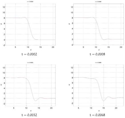
Figures 2–3 show a sequence of snapshots displaying the solution of Eq. (1) evolving from the initial condition chosen in the step-like (front-like) form
u(x, 0) =8 exp[−(x−5)2] forx ≥5 , u(x, 0)≡8 for x < 5 .
The idea is to help the solution curve acquire the step-like shape hinted by Fig. 1, although we realise that ultimate settled configuration of the solution will not depend of the initial condition. In our numerical experiments we chose not to transform the equation to the canonical form, in order to be able to adjust the coefficient values as necessary, for example to increase or reduce the energy release in the system in hope to achieve a self-sustained balance between the release and dissipation. The parameter values were: A =5, B= 1,C =1, the number of nodes 401, the length of thex-interval 10, time step 2·10−6. Thex-interval was constantly shifted to the right to follow the main kink, which, according to the initial shape, was to move to the right. When looking at Fig. 1(b), if one stretches thex-axis enough, the long shoulders would become nearly horizontal. In fact each shoulder could stretch to infinity on both sides of an isolated single step. Aiming at such a solution, we adopt the boundary conditions
t=0.0002 t=0.0008
[image:5.595.89.527.199.610.2]t=0.0032 t=0.0068
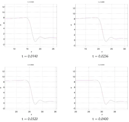
t=0.0140 t=0.0236
[image:6.595.91.527.198.610.2]t=0.0320 t=0.0400
The experiment showed that after some period of transitional evolution lasted from t0 = 0 to aboutt =0.03, the curve practically ceased changing in shape. Continuing the experiments further gave the same frozen shape of the solution moving with constant speed to the right. Looking at the solution displayed in Fig. 1(b) we see the same characteristic tale of ripples in front of the main kink. They were expected to form, caused by the high order of the dissipation acting in the system. Immediately in front of the main kink sits a shorter one, followed, as we look from left to right, by barely distinguishable smaller ripples. The height of the main kink relative to its neighbour is about 4:1 or a bit higher, for the both figures. The fact that the solution settles into a steady moving shape of correct proportions correlates with the earlier result.
4 CONCLUSIONS
We applied the 1D-IRBF numerical method to solve Eq. (1) simulating spinning combustion fronts and oscillations in certain class of reaction-diffusion systems. To our satisfaction, the method produced a similar shape of the settled travelling front as the earlier study [1]. We plan to use the 1D-IRBF approach to study more complicated regimes such as co-directed motion of several fronts, collision of counter-directed fronts etc.
REFERENCES
[1] Strunin, D.V. Autosoliton model of the spinning fronts of reaction. IMA J. Appl. Math. (1999)63:163–177.
[2] Strunin, D.V. Phase equation with nonlinear excitation for nonlocally coupled oscillators. Physica D(2009)238: 1909–1916.
[3] Mohammed, F.J, Ngo-Cong, D., Strunin, D.V., Mai-Duy, N. and Tran-Cong, T. Modelling dispersion in laminar and turbulent flows in an open channel based on centre manifolds using 1D-IRBFN method.Appl. Math. Model.(2014)38:3672–3691.
[4] Mai-Duy, N. and Tran-Cong, T. Numerical solution of Navier-Stokes equations using mul-tiquadric radial basis function networks.Int. J. Numer. Meth. Fluids(2001)37:65–86. [5] Mai-Duy, N. and Tanner, R.I. A collocation method based on one-dimensional RBF
inter-polation scheme for solving PDEs.Int. J. Numer. Meth. Heat Fluid Flow(2007)17:165– 186.
[6] Ngo-Cong, D., Mai-Duy, N., Karunasena, W. and Tran-Cong, T. Local moving least square- one-dimensional IRBFN technique for incompressible viscous flows. Int. J. Nu-mer. Meth. Fluids(2012)70:1443–1474.
[8] Ngo-Cong, D., Mai-Duy, N., Karunasena, W. and Tran-Cong, T. A numerical procedure based on 1D-IRBFN and local MLS-1D-IRBFN methods for fluid-structure interaction analysis.Comput. Model. Eng. Sci.(2012)83:459–498.
[9] Haykin, S. Neural networks: a comprehensive foundation. New Jersey: Prentice-Hall, (1999).
[10] Fasshauer, G.E. Meshfree approximation methods with Matlab. Interdisciplinary mathe-matical Sciences, Vol. 6., Singapore: World Scientific Publishers, (2007).
[11] Kansa, E.J. Multiquadrics – a scattered data approximation scheme with applications to computational fluid-dynamics – I. Surface approximations partial derivative estimates. Computers and Mathematics with Applications(1990)19:127–145.
[12] Kansa, E.J. (1990) Multiquadrics – a scattered data approximation scheme with applica-tions to computational fluid-dynamics – II. Soluapplica-tions to parabolic, hyperbolic and elliptic partial differential equations. Computers and Mathematics with Applications (1990)19: 147–161.
[13] Mai-Duy, N. and Tran-Cong, T. Numerical solution of differential equations using multi-quadric radial basis function networks.Neural Networks(2001)14:185–199.
[14] Mai-Duy, N. and Tran-Cong, T. Approximation of function and its derivatives using radial basis function networks.Appl. Math. Model.(2003)27:197–220.
[15] Mai-Duy, N. and Tanner, R.I. Solving high order partial differential equations with radial basis function networks.Int. J. Numer. Meth. in Engineering(2005)63:1636–1654. [16] Mai-Duy, N., See, H. and Tran-Cong, T. An integral-collocation-based fictitious domain
technique for solving elliptic problems.Communic. Numer. Meth. in Engineering (2008)
24:1291–1314.
[17] Mai-Duy, N. and Tran-Cong, T. A multidomain integrated radial basis function colloca-tion method for elliptic problems.Numer. Meth. for Partial Differential Equations(2008)
24:1301–1320.
[18] Mai-Duy, N. and Tran-Cong, T. Compact local integrated-RBF approximations for second-order elliptic differential problems.J. Comput. Phys.(2011)230:4772–4794. [19] Mai-Duy, N. and Tran-Cong, T. A compact five-point stencil based on integrated RBFs for
2D second-order differential problems.J. Comput. Physics(2013)235:302–321.