Modelling water allocation increases using climate predictions

(1)

University of Southern Queensland

Faculty of Health, Engineering and Sciences

Modelling Water Allocation Increases

Using Climate Predictions

A dissertation submitted by

Mr. Daniel Graham Verrall

In fulfilment of the requirements of

Bachelor of Engineering (Honours) (Civil)

(2)

ii

ABSTRACT

Water allocations in Australia often commence at the start of the year with less than 100% supply and rely on seasonal streamflows into dams throughout the year to meet demand. Therefore more than ever, water allocation models are used with forward planning in order to effectively manage water supply. This dissertation focuses on developing a water allocation model incorporating climate forecasts for Cressbrook Dam, a major water supplier for the regional town of Toowoomba.

After determining the best climate index of ENSO, the methodology focussed on identifying a relationship between streamflow and SOI on a monthly and seasonal scale and the creation of the water balance model. To apply the findings of these results, the use of three water management scenarios were then run through the water balance model using an extended streamflow sequence.

This analysis indicated that there was a significant correlation in the months of December to March which was further strengthened when looking at a seasonal scale. A consistently positive SOI observed in November suggested that there was a 100% chance that the dam level will substantially increase and this to develop alternative water management scenarios that raised restrictions when this SOI phase was observed.

By raising restrictions early, these management scenarios achieved a reduction of around 280 days from level 5 water restrictions which would have relieved the residents of Toowoomba during a major drought period. However, the raising of restrictions also resulted in lowering the dam level to a critical low volume.

(3)

iii

LIMITATIONS OF USE

The Council of the University of Southern Queensland, its Faculty of Health, Engineering & Sciences, and the staff of the University of Southern Queensland, do not accept any responsibility for the truth, accuracy or completeness of material contained within or associated with this dissertation. Persons using all or any part of this material do so at their own risk, and not at the risk of the Council of the University of Southern Queensland, its Faculty of Health, Engineering & Sciences or the staﬀ of the University of Southern Queensland.

(4)

iv

CERTIFICATION

I certify that the ideas, designs and experimental work, results, analyses and conclusions set out in this dissertation are entirely my own effort, except where otherwise indicated and acknowledged.

I further certify that the work is original and has not been previously submitted for assessment in any other course or institution, except where specifically stated.

Daniel Verrall

(5)

v

ACKNOWLEDGEMENTS

I would like to acknowledge the following people:

This project would not have been possible without the continual support from my family and friends who have been with me from my first day at the University of Southern Queensland.

(6)

vi

Table of Contents

ABSTRACT ... ii

LIMITATIONS OF USE ... iii

CERTIFICATION... iv

ACKNOWLEDGEMENTS ... v

Table of Contents ... vi

List of Figures ... x

List of Tables... xii

Nomenclature and Acronyms ... xiii

CHAPTER 1 INTRODUCTION ... 1

1.1 Background... 1

1.2 Aim and Objectives ... 2

1.3 Justification of Project ... 3

1.4 Dissertation Outline ... 3

CHAPTER 2 LITERATURE REVIEW ... 5

2.1 Introduction ... 5

2.2 Statistical Predictions for Water Allocation Increases ... 5

2.3 Climate Indices ... 6

2.3.1 Madden-Julian Oscillation (MJO)... 7

2.3.2 Tropical Cyclones ... 10

2.3.3 Atmospheric Blocking ... 12

2.3.4 East Coast Lows ... 14

2.3.5 Indian Ocean Dipole ... 15

2.3.6 Inter-Decadal Pacific Oscillation (IPO) ... 16

2.3.7 Southern Annular Mode (SAM)... 17

(7)

vii

2.3.9 Summary of Key Findings ... 24

2.4 Urban Water Storage Management – Risk ... 25

CHAPTER 3 METHODOLOGY ... 27

3.2 Hydrologic Analysis of Water Supply Systems ... 27

3.3 Water Balance Model ... 31

3.3.1 Behaviour Analysis ... 32

3.3.2 Storage volume at the end of the previous day (𝑺𝒕 − 𝟏) ... 33

3.3.3 Volume of stream inflow on day t (𝑸𝒕) ... 34

3.3.4 Volume of direct rainfall onto the dam on day t (𝑷𝒕) ... 34

3.3.5 Volume of water evaporated from the dam on day t (𝑬𝒕) ... 35

3.3.6 Volume of water infiltrated through seepage on day t (𝑰𝒕) .... 36

3.3.7 Volume of water drafted from the dam on day t (𝑫𝒕)... 37

3.3.8 Volume of water spilt on day t (𝑳𝒕) ... 37

3.3.9 Volume of Water Released from the Dam on Day t (𝑹𝒕) ... 38

3.3.10 Surface Storage Area... 39

3.4 Streamflow and ENSO Relationships ... 39

3.4.1 Monthly Streamflow and ENSO Relationships ... 40

3.4.2 Seasonal Streamflow and ENSO Relationships ... 41

3.4.3 Seasonal Cumulative Probability Distributions ... 41

3.5 Combined Water Balance Model with ENSO Relationships ... 42

3.6 Scenarios... 43

3.6.1 Scenario 1 ... 43

3.6.2 Scenario 2 ... 45

3.6.3 Scenario 3 ... 46

3.6.4 Development of Streamflows for Scenarios ... 47

(8)

viii

4.2 Monthly Streamflow and ENSO Analysis ... 49

4.3 Seasonal Streamflow and ENSO Analysis ... 51

4.4 Seasonal Cumulative Probability Distribution Analysis ... 52

4.5 Cumulative Probability Distribution Analysis of End of Season Storage Levels ... 55

4.5.1 90% Starting Storage Capacity ... 56

4.5.5 Summary of End of Season Storage Levels ... 60

CHAPTER 5 RESULTS FOR WATER MANAGEMENT SCENARIO ANALYSIS ... 61

5.2 Extended Streamflow Sequence Development and Validation ... 61

5.2.1 Relationship and Validation of Streamflows between Cressbrook Dam Site and Tinton ... 61

5.2.2 Relationship and Validation of Streamflows between Cressbrook Dam Site and Rosentretters Crossing ... 65

5.2.3 Extended Streamflow Gap Analysis ... 66

5.3 Water Management Scenarios ... 68

5.4 Discussion of Key Results ... 72

CHAPTER 6 CONCLUSION AND FUTURE WORK ... 78

6.2 Achievements ... 78

6.3 Recommendations and Future Work ... 80

CHAPTER 7 REFERENCES ... 81

(9)

ix APPENDIX A – PROJECT SPECIFICATION ... 87 APPENDIX B – PROJECT PLAN TIMELINE ... 88

APPENDIX C – MONTHLY STREAMFLOW AND SOI

(10)

x

List of Figures

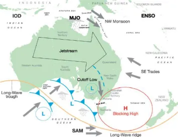
Figure 1: The Main Climate Indices Driving Rainfall Variability in Australia

(Risbey et.al, 2009) ... 7

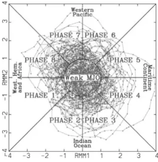
Figure 2: The Eight Different Phases and Locations of the MJO (Zhang, 2013) ... 9

Figure 3: East Queensland Tropical Cyclones from 1970 to 2004 (BOM, n.d.) ... 11

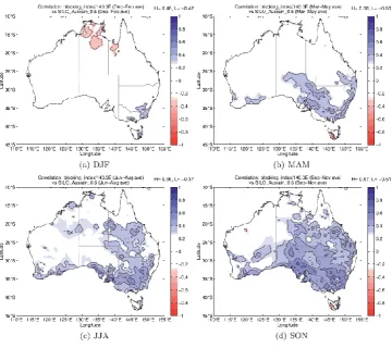
Figure 4: Correlation between Blocking and Rainfall in Different Australian Seasons (Risbey et.al, 2009) ... 13

Figure 5: East Coast Lows (green) move up the coastline of NSW (Klingaman, 2012) ... 14

Figure 6: a) IOD correlation to rainfall with the presence of ENSO b) IOD correlation to rainfall without the presence of ENSO (Risbey et.al, 2009) . 16 Figure 7: Correlation between SAM and rainfall throughout Australia in different seasons (Risbey et.al, 2009) ... 18

Figure 8: SOI readings in Australia in the past seven years (BOM, 2015) .. 21

Figure 9: ENSO correlation between SOI and rainfall within Australia over four seasons (Risbey et.al, 2009) ... 21

Figure 10: Forecast Hit Rate for the SOI Index since 2000 (Stone, 2011) .. 23

Figure 11: Relationship between storage, yield and reliability (Lough, 2008) ... 31

Figure 12: Inflows and Outflows from a Reservoir (Lough, 2008) ... 32

Figure 13: Scenario 2 Decision Tree ... 45

Figure 14: Scenario 2 Decision Tree ... 46

Figure 15: Seasonal Streamflow and SOI Relationships ... 51

Figure 16: Cumulative Probability Distribution Graph for Cressbrook Creek ... 54

Figure 17: Cumulative Probability Distribution at 90% Starting Level ... 56

Figure 21: Tinton Streamflow vs Dam Site Streamflow (<3000 ML) ... 63

(11)

xi Figure 23: Water Storage of Cressbrook Dam 1952-2015 with Three Different

Water Management Strategies ... 69

Figure 24: Water Storage of Cressbrook Dam 2006-2015 with Three Different Water Management Strategies ... 71

Figure 25: SOI and Streamflow Relationship for January ... 89

Figure 26: SOI and Streamflow Relationship for February ... 89

Figure 27: SOI and Streamflow Relationship for March ... 90

Figure 28: SOI and Streamflow Relationship for April ... 90

Figure 29: SOI and Streamflow Relationship for May ... 91

Figure 30: SOI and Streamflow Relationship for June ... 91

Figure 31: SOI and Streamflow Relationship for July ... 92

Figure 32: SOI and Streamflow Relationship for August ... 92

Figure 33: SOI and Streamflow Relationship for September ... 93

Figure 34: SOI and Streamflow Relationship for October... 93

Figure 35: SOI and Streamflow Relationship for November... 94

Figure 36: SOI and Streamflow Relationship for December ... 94

Figure 37: All Dam Storage Responses with a Starting level of 90% ... 95

(12)

xii

List of Tables

Table 1: Climate Index to be used in the analysis for each season ... 24

Table 2: Monthly average rainfall for Cressbrook Dam ... 35

Table 3: Monthly Pan Evaporation for Cressbrook Dam... 36

Table 4: Surface Area of Cressbrook Dam depending on storage volume .. 39

Table 5: Water Restrictions in Place by TRC ... 44

Table 6: Average Correlation Values for Each Month ... 49

Table 7: Monthly Streamflow Totals ... 50

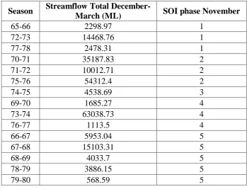
Table 8: Streamflow Totals According to SOI Phase in November ... 53

Table 9: Dam volume increases and decreases at 100% Probability ... 60

Table 10: Missing Data Gaps Summary ... 66

(13)

xiii

Nomenclature and Acronyms

ENSO - El Niño Southern Oscillation

MJO - Madden-Julian Oscillation

BOM - Bureau of Meteorology

SOI - Southern Oscillation Index

ECL - East Coast Lows

IOD - Indian Ocean Dipole

SST - Sea Surface Temperature

DMI - Dipole Mode Index

IPO - Inter-Decadal Pacific Oscillation

PDO - Pacific Decadal Oscillation

SAM - Southern Annular Mode

EOF - Empirical Orthogonal Functions

EMO - ENSO Modoki Index

DNRM - Department of Natural Resources and Mining

ML - Megalitres

(14)

(15)

1

CHAPTER 1

INTRODUCTION

1.1 Background

Australia has an extremely variable climate which can change from prolonged drought to flash flooding within a short period of time. Therefore it is important that water allocation models can accurately predict when water usage needs to be tightened and relaxed. While there are numerous literature regarding the changing climate of the earth, there is little in the way of how this knowledge can be applied to solving real world problems. The use of seasonal climatic data to aid in predicting short-term water allocations is one such problem that can be addressed. This proposal suggests a possible case study for developing a water allocation model for Cressbrook Dam, which is the major water supplier to the regional town of Toowoomba.

As Australia’s second largest inland city, the expanding city of Toowoomba faces the challenge of finding more water resources to keep up with increasing demand. As a regional city, rainfall varies significantly within the Darling Downs from season to season. Due to this variability, Toowoomba receives much lower annual rainfall totals than other coastal south-east Queensland cities such as Brisbane, Sunshine Coast and Gold Coast. A rainfall comparison between Toowoomba (mean = 720.3 mm) and Brisbane (mean = 1011.7 mm) shows that on average the capital city receives nearly half a metre more in annual rainfall (BOM, 2013).

(16)

2 - Harsh level 5 water restrictions

- The proposal to use recycled water for drinking purposes

- The eventual construction of the pipeline from Wivenhoe Dam to Cressbrook Dam

After the 2011 January floods and all of Toowoomba’s dams were refilled to capacity, the Toowoomba Regional Council (TRC) decided to keep the region on permanent conservation water restrictions. Being one of the only places throughout Australia to use such permanent conservation water measures means that it has been identified that water availability will be an ongoing issue for the region in the future.

1.2 Aim and Objectives

Therefore there was an opportunity to investigate whether climate indices can help water managers in their forward planning and decision-making in regards to future streamflow forecasts. With this in mind, the primary aim of this research project is to provide a functioning water allocation model that can predict with short-term accuracy the likely increases and shortfalls in water availability for Cressbrook Dam using an appropriate climate indicator. In order to achieve this primary aim, three key objectives were identified and are listed below:

- Find a significant relationship between the most influential climate index and streamflow

- Incorporate climate-streamflow relationships into a working water balance model

(17)

3 1.3 Justification of Project

The severe drought from 2000 to 2010 resulted in Toowoomba facing a water supply emergency with the combined dam level dropping to an all-time low of 7.8% in February 2010. This affected the livelihoods of many residents of the region in regards to water usage including myself. For the water supply systems in the area to get that critically low, it raised many questions as to why this occurred. Was it purely due to a major drought event, or could the management of the urban water supplies have been better managed so that there was not as much pressure placed on the community with its water consumption. It’s for this reason that the use of climate indices were investigated to determine whether forecasting could have helped in the past and can be used in the future.

1.4 Dissertation Outline

There are 6 main chapters in this dissertation including the introduction. A short outline for each chapter is detailed below:

Chapter 2 – Literature Review

The literature review discusses why historical statistical approaches are used in the dissertation, reviews and assesses the best climate driver which affects the streamflows of Cressbrook Creek and discusses the risks associated with urban water supply management.

Chapter 3 – Methodology

(18)

4 three different water management scenarios, where water restrictions are based off the relationships found between streamflow and climate indices.

Chapter 4 – Results for Statistical Streamflow Forecast Model

This chapter shows the results on the best linear relationships between streamflow and climate indices and uses these results to develop cumulative probability distribution graphs for a range of different starting dam levels.

Chapter 5 – Results for Water Management Scenario Analysis

This chapter explains how the extended streamflow sequence was created and validated as well as the key results found from running the three different scenarios through the water balance model.

Chapter 6 - Conclusion

(19)

5

CHAPTER 2

LITERATURE REVIEW

2.1 Introduction

This review will discuss the use of statistical models which use the concept of stationarity to link historical streamflow data to associated climate indices to provide an adequate water allocation model. An investigation into the relationship between streamflow data and climate predictions will then be examined in the aim to determine a climate index that will have the largest impact on the Cressbrook Creek catchment area. Lastly a discussion will review the risk management of urban water supplies and water resource managers’ approaches towards urban water supply.

2.2 Statistical Predictions for Water Allocation Increases

Any type of prediction model can be produced from either complex dynamic numerical approaches or based on historical statistical data. While dynamic models are the preferred choice in today’s world due to climate change, historical statistical data for predicting future rainfall events are still widely used through Australia. However there are some research papers in the past have which have looked at using climate models for streamflow forecasting within Australia (Chiew et.al 1998, Everingham et.al 2008). These papers make use of statistical approaches, where climate and streamflow events of the past are used as the basis for future predictions (Baillie & Brodie, 2011).

(20)

6 dependent on the length and quality of historical streamflow and SOI data. The assumption of statistical stationarity also poses the problem of current and future conditions falling outside the limits of historical data range where both the risk and accuracy of forecasting is unknown. However, statistical approaches have the advantage of finding a direct relationship between streamflow and large climate drivers and its relative ease of use means that such approaches are well developed around Australia (Baillie & Brodie, 2011). Therefore statistical approaches is seen to be appropriate to use throughout this study.

2.3 Climate Indices

(21)

[image:21.595.116.472.74.347.2]

7 Figure 1: The Main Climate Indices Driving Rainfall Variability in Australia (Risbey et.al,

2009)

2.3.1 Madden-Julian Oscillation (MJO)

(22)

8 Zhang (2005) explains that the effects that the MJO has on Australia’s weather, particularly in Queensland depends on the state or phase of other known climate phenomena’s such as ENSO and their combined effects can result in significant weather events. The simplest observations made about the MJO is that the event features a large scale eastward moving centre of strong deep convection which is representative of an active stage of the event. The inactive stage is where both and east and west regions are diverted by weak convection and precipitation. Both of these phases of the MJO are linked by air circulations that occur vertically through the lower atmosphere. In the troposphere where all weather events occur, strong westerly and easterly winds coincide with their direction with a large-scale convective centre in the middle of the system. Once in the upper troposphere, the circulation of air will cause the winds to reverse directions. The connection between large air circulation and convective centre propagating slowly eastward at an average of 5 metres per second is essential to the characteristics of the MJO.

(23)

9 is a geographic preference and a distinguishable multiscale structure (Zhang, 2005).

[image:23.595.217.376.543.706.2]

According to Risbey et.al (2009), the MJO is split into eight unique phases based on the different patterns of variability of convection and zonal winds within the system at latitudes close to the equator (Figure 2). These different patterns are used to describe the current location of the MJO and can be analysed for future predictions of the system. As claimed by Risbey et.al (2009), statistical and historical data analysis has shown that the strongest association that the MJO has with the Australian climate is in the northern part of Australia. As highlighted by Figure 1, the location of the MJO in phases 5 and 6 coincide with strong rainfall events occurring across the northern tropics of Australia during the monsoon season. Wheeler et.al (2009) suggests that weekly rainfall in northern Australia can increase more than three times with the convectively active MJO phase compared to its suppressed phase. There is also studies conducting which have shown that MJO can be influenced and can interact with ENSO. Wet MJO-related events are seen to have comparable characteristics to La Niña and vice versa with El Niño weather events. However overall analysis of the analysis between the two climate indices shows that ENSO is the dominant climate index and that the relationship between rainfall and ENSO is dependent on the activities of the MJO.

(24)

10 Studies from Wheeler et.al (2009) analyse the possible impacts that the MJO has on Australia rainfall in extratropical regions and other locations other than the northern tropics and also whether its impacts vary with different seasons. Findings were shown that a winter season rainfall response to the MJO was evident along the Queensland coast, caused by the systems trade winds. However in all other places in different places, the MJO’s effect is inconsistent and only found to have minimal correlation in localised areas. Although it is suggested that these responses are due to continental circulation, it is more likely that southern blocking may have a stronger presence in influencing extratropical regions such as the Darling Downs area.

2.3.2 Tropical Cyclones

According to Klingaman (2012), an average of four tropical cyclones per year form of the Queensland coast in the Coral Sea during the season between January to March. Further historical analyses from Klingaman (2012) indicates that on average at least one or two of these tropical cyclones will impact make landfall and impact the Queensland coast each year. Inter-annual variability is also shown to exist between the number of land falling cyclones with many years having no land falling cyclones and other years having up to three. Importantly, there is evidence from Lough (1991) to suggest that there is a positive correlation showing that years with above average annual mean rainfall coincide with years where there was a greater number of land falling tropical cyclones. These studies have complementary findings to back up what is already thought to be known, there is a higher chance of more extreme rainfall events occurring when there is an increase in the number of land falling cyclones within the Queensland region.

(25)

11 coastline of Queensland. The opposite effect is experienced during the La Niña where the spawn of tropical cyclones are closer to the Queensland coast, therefore increasing the chances of cyclones having an effect on rainfall anomalies. Variation of the strength and locations of tropical cyclone have also been attributed to the behaviour of the monsoon trough. The monsoon trough also works in unison with the ENSO climate, but affecting the generation of cyclones through differences in zonal winds (Klingaman, 2012).

[image:25.595.183.413.548.749.2]

Importantly, the impact of rainfall variability from tropical cyclones is mostly associated with affecting tropical parts of the country. Extratropical regions such as the focus region of the Darling Downs seldom has tropical cyclone influence. The last time that a tropical cyclone had a major impact on the Darling Downs region was in 1974 when Tropical Cyclone Wanda which crossed the coast near Maryborough (Office of Economic and Statistical Research, 2009). As the region of focus is inland, tropical cyclones are more likely to affect the Darling Downs as a rain depression rather than a cyclone. As explained by the Bureau of Meteorology (n.d.), tropical cyclones have a tendency to follow the Queensland coastline before moving safely away from the continent into the Pacific Ocean (as shown in Figure 3). Therefore cyclone activity if any, has a greater impact on coastal cities within south-east Queensland such as Brisbane then in the Toowoomba region.

(26)

12 2.3.3 Atmospheric Blocking

It is now well recognised that atmospheric blocking is an important climate driver for both southern and eastern parts of Australia. Blocking is often associated with blocking ‘anticyclones’ which areas of slow moving high pressure systems that form due to the presence of atmospheric longwave patterns. The formation of these anticyclones occur most frequently in the Tasman Sea and the Southern Ocean with the most frequent occurrence being in the southeast of Australia during winter. Blocking can occur at any time of the year, however blocks form mostly between the months of April to August. The cause of atmospheric blocking is linked with the splitting of upper atmospheric westerly winds into two distinguishable states. The degree of this splitting in the atmosphere is represented by the BOM by a simple blocking index. An expression is used to calculate a monthly blocking index at a constant longitude of 140°E. The BOM uses this longitude value as it is found to be a common location where blocking occurs and affects the weather in Australia (Risbey et.al, 2009).

(27)

[image:27.595.119.480.169.489.2]

south-13 eastern part of Australia. Figure 4 shows that there is a positive correlation between the blocking index (using 140°E) and Australian rainfall for all seasons except for summer.

Figure 4: Correlation between Blocking and Rainfall in Different Australian Seasons (Risbey et.al, 2009)

(28)

14 Atmospheric blocking and cut-off lows affect the rainfall variability in the Darling Downs region from the months of June to November, with a noticeably apparent positive correlation shown in Figure 4. For south-eastern Queensland, atmospheric blocking is considered to be the dominant remote driver of spring rainfall over other climate drivers including the SOI, IOD and the SAM. However the examination of the link between blocking and rainfall variability within Queensland has not be extensively researched compared to other states such as New South Wales and Victoria where blocking has the greatest impact (Klingaman, 2012).

2.3.4 East Coast Lows

[image:28.595.126.462.501.747.2]

East coast lows (ECLs) are areas of closed circulation that form low pressure systems near the eastern coast of Australia and move parallel along the coastline (Figure 5). Although east coast lows can form at any time of the year, its most significant impact on Queensland is during the winter. During this time period, ECLs can produce heavy rainfall events when it associates with high pressure systems which are found to be at the most northern position (Pepler et.al, 2014).

(29)

15 Klingaman (2012) further explains that substantial inter-annual variability exists in the number of ECLs that affect Queensland with range between 0 and 5 ECls occurring each year. It also been found that there is no significant correlation that exists between ECLs and SOI phases. However there was a detection of correlation between ECLs and ENSO transition phases with a shift from El Niño to La Niña resulting in more ECLs and vice versa. There is no evidence however to connect the physical mechanism between ENSO shifts and ECLs. Overall ECLs are only responsible for rainfall between 3 to 5 days each year during the winter period, with its impact on rainfall variability mostly examined to be in the states of New South Wales and Victoria.

2.3.5 Indian Ocean Dipole

The Indian Ocean Dipole (IOD) is major climate driver for countries within the boundary of the Indian Ocean. The IOD is known to be a major component of sea surface temperature (SST) variability in the Indian Ocean near the equator. It is thought that the sea surface temperatures in the equatorial Indian Ocean co-varies with that in the tropical Pacific Ocean during ENSO and has a major impact on rainfall variability within Australia. Variations of SSTs in the Indian Ocean, are responsible for playing a primary role in rainfall variability in the southern regions during austral winter and early spring (Cai et.al, 2011).

(30)

16 A measure of the IOD is the dipole mode index (DMI), which is the difference in SST’s between the equatorial western Indian Ocean and the equatorial south-eastern Indian Ocean. As Figure 5a shows there is statistically significant correlation between Australian rainfall and the DMI for the peak IOD period between the months of June to October across mainly the southern part of Australia, but also effect parts of Queensland. However when the effect of ENSO is removed from the IOD, its independency shows that there is near to zero correlation between the IOD and rainfall in Queensland (Figure 5b). Studies as explained by Klingaman (2012), also suggest that there is no important correlation between Indian Ocean SSTs and rainfall within south-east Queensland. Therefore the IOD has little to no impact on the rainfall variability of the Darling Downs region.

Figure 6: a) IOD correlation to rainfall with the presence of ENSO b) IOD correlation to rainfall without the presence of ENSO (Risbey et.al, 2009)

2.3.6 Inter-Decadal Pacific Oscillation (IPO)

(31)

17 explain lower frequency SST variability and are part of a larger system described as the Inter-decadal Pacific Oscillation (IPO). During the twentieth century there has been three phases of IPO that have been identified: a positive phase from 1922 to 1944, a negative phase from 1946 to 1977 and another positive phase from 1978 to 1998. During these phases it is thought that the IPO has a role in modulating inter-annual ENSO related climate rainfall variability over Australia. Through the use of teleconnection analysis, relationships with ENSO are seen to be varied with areas such as New Zealand showing strong teleconnections for positive IPO periods whereas in some Pacific areas showing weaker teleconnections (Power et.al, 1999).

As explained by Klingaman (2012), during the positive IPO phase of 1922 to 1944, both ENSO and Queensland became uncorrelated. The positive phase of the IPO, SSTs are found to be warmer in the Eastern Pacific and cooler in the extratropical West Pacific Ocean. Within this time period it was discovered that Queensland rainfall became less variable and spatially coherent. Salinger et.al (2001) claimed findings that suggested that the positive IPO phase was the result of a weakening in the ENSO Australian rainfall variability. This means that when positive IPO is currently present, modelling of the ENSO signal appears to be much more difficult and unpredictable. Therefore there is a limited understanding of the mechanisms that produce a weakening of the ENSO related rainfall variability in Queensland during positive IPO phases and also little knowledge besides its influence of the ENSO climate driver.

2.3.7 Southern Annular Mode (SAM)

(32)

18 zonal winds that are higher than usual in the mid-latitudes and lower than usual in the high-latitudes and vice versa for the negative SAM phase. There is also been evidence to suggest that there is a link between SAM variability and the synoptic behaviour of Australia.

[image:32.595.153.442.471.726.2]

A way of defining the SAM climate system is using the difference between monthly zonal mean sea level pressures at 40 and 65°S latitude to form the SAM index. Using station pressures dating back to 1957, the SAM index is calculated on projecting daily 700 hPa heights onto empirical orthogonal functions (EOFs) of monthly mean 700 hPa heights. When correlating the index with rainfall variability in Australia, it was found that the SAM system only accounts for around 15% of weekly rain variance in only the south-western and south-eastern parts of Australia (Hendon et.al, 2007). Risbey et.al (2009) further explains that the positive phase of SAM has been linked to a reduction of rainfall in southern Australia particularly in winter months. However in spring, positive SAM is associated with increased rainfall mostly on the southeast coast of New South Wales but also in the southwest of Western Australia (Figure 7).

(33)

19 Overall there are only very weak relationships between the SAM system and rainfall within south-eastern Queensland. As from Figure 7, spring appears to be the season with the most correlation, but this correlation shows to have a greater impact in New South Wales than Queensland. The correlation between SAM and rainfall in spring is most likely explained by the presence of an enhanced onshore flow that occurs during that time period (Klingaman, 2012).

2.3.8 El-Nino Southern Oscillation (ENSO)

(34)

20 tend to be below average and rainfall patterns are more widespread than that of El Nino.

(35)

[image:35.595.139.459.66.296.2]

21 Figure 8: SOI readings in Australia in the past seven years (BOM, 2015)

The Bureau of Meteorology and Long Paddock (operated by the Science Delivery Division of the Department of Science, Information Technology and Innovation (DSITI) and provided by the Queensland Government) have SOI recordings dating from 1876 to present. In Figure 9 below, Risbey et.al (2009) use SOI data ranging from 1889 to 2006 with correlation to rainfall over the four different seasons of the year.

[image:35.595.149.442.476.734.2]

(36)

22 From above it seen that there is a clear correlation between ENSO and rainfall in the eastern and north-eastern parts of Australia particularly during winter and spring. This supports claims by Klingaman (2012) that tropic rainfall in Australia is linked to SSTs and that ENSO is responsible for much of the inter-annual rainfall variance the in the extratropics. Studies suggest that the strongest SOI correlation with rainfall in Queensland occur during the spring months of October and November. Very few regions in Queensland however are shown to have a statistically insignificant relationship between rainfall and SOI. ENSO is known by many sources (Klingaman, 2012; McBride & Nicholls, 1983) to be weak and incoherent throughout the autumn season and is referred to as the ENSO “predictability barrier”.

Due to the ENSOs dominance in driving the climate of eastern Australia, it has been explained by previous climate index sections above that ENSO can modulate rainfall variability on synoptic and sub-seasonal scales, as well having effects on other climate drivers such as the generation of tropical cyclones, MJO, IOD and blocking. ENSO also remains to be seen as the dominant climate driver in Queensland due to the system which can act over many different timescales. While Klingaman (2012) explains that ENSO has the greatest impact on Queensland rainfall at the seasonal or inter-annual level, there is also evidence provided by Risbey et.al (2009) that claim that ENSO causes considerable multi-decadal variability in Australia rainfall patterns.

(37)

23 the SOI is a positive value and sea surface temperatures in the Pacific Ocean are lower than average (and vice versa). In terms of accuracy, a lag correlation analysis is shown to have the most potential in forecasting future events. Indicators of ENSO can be used to successfully forecast rainfall throughout eastern Australia in the spring months and summer months in north-eastern Australia.

With so many climate patterns and systems that exist and interact with each other on varying timescales, applying these climate drivers to real life situations becomes very complex. However the Bureau of Meteorology (2016), uses a number of different climate and synoptic drivers such as SOI, SSTs, trade winds, cloudiness near the dateline and the IOD to deliver a seasonal forecast for the next couple of months. In the seasonal outlook, the Bureau still regards ENSO as the core driver of climate for Australia.

(38)

24 Figure 10 above explains the use of forecast hit rates using the SOI index from 2000. From this figure it is seen that the forecast success rate (recognised consistent ENSO rainfall relationships) in Queensland are mainly above 50%. The forecast skill of the ENSO is produced by the ‘SOI phase system’ which is applied to many agricultural and urban water supply situations which will be explained in the following sections.

2.3.9 Summary of Key Findings

A number of different climate indices were investigated in order to determine which index has the most influential effect on the Darling Downs region. The following Table (Table 1) summarises the key findings by listing the climate index that has the greatest impact on the region in each individual season of a year.

Table 1: Climate Index to be used in the analysis for each season

Season Climate Index to be Used

Summer

(December-January-February) ENSO

Autumn (March-April-May) ENSO

Winter (June-July-August) ENSO

Spring

(September-October-November) ENSO

(39)

25 has the strongest relationship between itself and rainfall and can be forecasting with the highest confidence levels in both the major seasons of winter and summer.

The most dominant climate index in the transitional seasons of autumn and spring are more unclear with ENSO have its weakest influence in autumn. However there is no other clear climate index that dominates the season of autumn and therefore ENSO was also chosen for this season. For spring there is reason to believe that atmospheric blocking is the most dominant influencer on climate. However Klingaman (2012) also explains that the relationship between rainfall and atmospheric blocking in Queensland has not been extensively researched and cannot be ascertained with high confidence. Therefore overall the climate index of ENSO was used within this investigation.

2.4 Urban Water Storage Management – Risk

(40)

(41)

27

CHAPTER 3

METHODOLOGY

3.1 Introduction

This chapter details the importance of dam storages, and the relationships between its draft, storage, yield and reliability. It will then discuss the development of a water balance model for Cressbrook Dam which includes the inputs of streamflow and rainfall, and the outputs of evaporation, infiltration, water demand, spill over the top of the dam and water releases downstream. The next stage describes the linear regression analysis used to determine the best relationship and lag increase between SOI and streamflow data for Cressbrook Dam on both a monthly and seasonal scale. Lastly combining ENSO into the water balance model the development of three different water management scenarios will be discussed along with how the extended streamflow sequence was developed for the water balance model.

3.2 Hydrologic Analysis of Water Supply Systems

Estimations of volume runoff from a catchment are often required for civil engineers for a number of different applications. One of the most important reasons is for the design of containment systems, in particular dams which are able to store water over a relatively long periods of time. In today’s modern world the demand for a city’s water supply is an essential part of establishing a functional community. In order to meet the water demand of the city, water volumes of surface runoff are needed for the assessment of dam storages and urban water supply management so that the required amount can be delivered to urban, agricultural and industrial water users (Brodie, 2015).

(42)

28 annually totals. The timescale used depends on the application and is expressed as a water volume over a certain time period. There are a number of ways that runoff volumes can be determined which mostly depends on the availability of measured streamflow data. One of the procedures used involves uses a water balance model when there is limited or no streamflow records or gauging stations available, however there would be less confidence in the accuracy of the predicted flow volumes made. There are also other runoff volume calculations that can be used for a variety of different timescales such as the average annual runoff produced from a catchment for a broader water resources approach as well as a runoff volumes for an individual storm event which is calculated using the volumetric runoff coefficient.

However within this investigation modelled streamflow data in the form of ML/day was obtained by the Department of Natural Resources and Mining (DNRM) over a number of years. Once large datasets of streamflow data are recorded over a long period of time such as TRC’s, other important hydrological values can be assessed using storage behaviour analysis. Toowoomba’s water supply from Cressbrook, Perseverance and Cooby Dam are designed to increase the amount of water available, store water when flows and demand are sufficiently large and be able to provide water when streamflows into the dams are sufficiently low. If streamflows into the reservoir are large, they may be sufficient enough to fill the reservoir causing it to spill the uncontrolled flow of water over the top of the reservoir spillway.

(43)

29 is contained and controlled with engineering structures such dams and reservoirs which are needed to provide water to satisfy the large demands of agricultural, industrial and domestic needs over a large area. These systems are often associated with having carry over storages where water can be held over many seasons so that there is supply available when streamflows coming into the reservoir are below average. Cressbrook Dam is therefore seen to be a regulated system that uses carry-over storages to satisfy water demands and this will be known throughout the analysis of the report (Lough, 2008).

As explained by Linsley & Franzini (1964), another aspect of reservoirs in the minimum operating level which is taken into consideration in its design which ensures that it will never go completely dry. The minimum operating level is usually calculated by a certain volume of water that remains at the bottom of the reservoir with any volume taken below this level known as the dead storage. While the dead storage takes water from below operating level, the active storage is the volume in a reservoir that used during normal operations. The active storage is any amount of water that is between the full supply and the minimum operating level of the reservoir.

Three important terms that are commonly associated with water supply and storage are a dam’s yield, draft and reliability. Both yield and draft are used interchangeably and refer to the average volume of water that is supplied by the dam to satisfy water demand needs over a certain period of time. The yield of dam is also often set to meet water demands at a specified level of reliability (Linsley & Franzini, 1964). As discussed by Brodie (2015), the reliability of a dam is the proportion of time that a target demand can be met and is expressed by the following equation.

𝑅(%) =𝑁𝑠

𝑁_𝑡× 100

Where

(44)

30 And 𝑁_𝑡 = the total number of time periods

Therefore as expected, the calculation of yield and in turn reliability depends on a number of factors such as streamflow regimes, water demand patterns, water supply system characteristics, evaporation from reservoirs and most importantly the possible factor of climate changes which is being investigated in this report. As claimed by Lough, (2008) It is clear that there is a link between storage, yield and reliability and that a relationship can be derived between the three. This is best explained by the difference between a regulated and unregulated system. If an unregulated system harvests water from an uncontrolled stream then the reliability and water supply will be relatively low and if a flood occurs, the yield will be relatively high for a short period of time. In a regulated system however, the presence of a storage capacity will increase both the yield and reliability. Therefore the three terms can be formed into the following equations to represent the relationship between each other and described by Figure 11.

𝛼 =𝐷

𝑄̅ 𝑎𝑛𝑑 𝑆

∗ ₌ 𝑆

𝑄̅

Where

𝛼 = Draft ratio (%)

𝐷 = Draft (ML)

𝑄̅ = Mean annual flow (ML)

𝑆∗ = Storage ratio

(45)

31 Figure 11: Relationship between storage, yield and reliability (Lough, 2008)

From this graph, it is shown that the storage capacity ratio is plotted on the x-axis against the draft ratio in the y-x-axis. The two different lines represent both a regulated and unregulated system with differing reliabilities. It is seen that as the storage ratio increases (a function of storage capacity over the mean annual flow) the draft ratio (a function of yield over the mean annual flow) also increases at a decreasing rate. For a given storage capacity of a dam, it is seen that as the reliability increases, the yield decreases due to less water being harvested (Lough, 2008).

3.3 Water Balance Model

(46)

32 3.3.1 Behaviour Analysis

As suggested by Brodie (2015), in a storage behaviour analysis the application of a water balance equation are used to determine both the dam yield and reliability. At its simplest form, the change in storage volume in a reservoir is equal to the difference between the inflow and outflow of the system which is consistent with the conservation of mass. However a proper and complex water balance model accounts for a number of different parameter as seen in Figure 12 below.

Figure 12: Inflows and Outflows from a Reservoir (Lough, 2008)

From this diagram, the following water balance equation can be formed:

𝑆_𝑡 = 𝑆_𝑡−1+ 𝑄_𝑡+ 𝑃_𝑡− 𝐸_𝑡− 𝐼_𝑡− 𝐷_𝑡− 𝐿_𝑡− 𝑅_𝑡

Where

𝑆_𝑡 = Storage volume on day t (ML)

𝑆𝑡−1= Storage volume at the end of the previous day t-1 (ML)

𝑄𝑡 = Volume of stream inflow on day t (ML)

𝑃_𝑡 = Volume of rainfall that falls directly onto the dam on day t (ML)

𝐸_𝑡 = Volume of water evaporated from the dam on day t (ML)

𝐼_𝑡 = Volume of water infiltrated through seepage on day t (ML)

(47)

33

𝐿𝑡= Volume of water spilt on day t (ML)

𝑅𝑡 = Volume of water released on day t (ML)

According to Lough (2008), the water balance equation shows that there are two main sources of inflow into the dam which are the natural streamflows and the direct rainfall on the dam site as well as the storage that is already present from the previous day. The outputs of the water balance equation include evaporation, infiltration, water draft, the spillage over the top of the dam and the environmental releases from the dam. The determination of each of these parameters will be further discussed in the sections below as well as how the surface area of the water held by the dam can affect the overall volume of the storage.

3.3.2 Storage volume at the end of the previous day (𝑺𝒕−𝟏)

(48)

34 3.3.3 Volume of stream inflow on day t (𝑸_𝒕)

The volume of streamflow running into the dam site is the main source of storage volume increase. Streamflow data from Cressbrook Creek was sourced from DNRM, with volumes in the form of ML/day taken to determine the inflow and increase of the storage dam volume. Although not ideal, the only streamflow data from DNRM is from a closed gauging station with records lasting from 1965 to 1981 and providing 16 years of usable data.

3.3.4 Volume of direct rainfall onto the dam on day t (𝑷𝒕)

(49)

[image:49.595.150.446.107.366.2]

35 Table 2: Monthly average rainfall for Cressbrook Dam

Month Average Monthly Rainfall (mm/month)

January 121.3

February 121.9

March 70.1

April 38.5

May 56.6

June 34.7

July 25.3

August 26.1

September 36.6

October 57.6

November 74.2

December 107.4

3.3.5 Volume of water evaporated from the dam on day t (𝑬_𝒕)

(50)

36 simplistic nature and the requirement of only small amounts of data. Monthly pan factors have been computed for 29 stations located throughout Queensland. The closest station to Cressbrook Dam is Gatton as explained by Queensland Government (2008), which gives average monthly values in mm which was then converted into equivalent daily evaporation values as shown in Table 3 below.

Table 3: Monthly Pan Evaporation for Cressbrook Dam

Month Monthly Pan Evaporation (mm/month)

January 201

February 163

March 163

April 130

May 96

June 84

July 92

August 116

September 152

October 182

November 197

December 213

3.3.6 Volume of water infiltrated through seepage on day t (𝑰_𝒕)

(51)

37 3.3.7 Volume of water drafted from the dam on day t (𝑫_𝒕)

Toowoomba’s main three urban water suppliers are from Cooby Dam, Perseverance Dam (upstream) and Cressbrook Dam (downstream). The volume of water that is drafted from each of these dams depends on a number of different factors. These factors include population, water restrictions, and the size capacity of the dam itself. Cressbrook Dam is the largest supplier of urban water with a maximum capacity of 81842 ML. Currently, water restrictions within Toowoomba are a part of permanent conservation measures. As explained by Toowoomba City Council (2006), the average consumption under these measures is 250 L/p/d and is used as the base volume of water drafted in the water balance model. The current population according to Boyd (2014) is 135,000 people. Therefore multiplying the water consumption by the population gives the total demand required for Toowoomba each day. However taking into consideration that water is drafted from all three dam sources, it was determined that Cressbrook Dam (as the largest supplier) accounts for approximately 60% of the daily demand (Toowoomba City Council, 2006). Therefore applying a factor of 0.6 to the total daily demand a draft value of 20.25 ML was used for the water balance model.

3.3.8 Volume of water spilt on day t (𝑳𝒕)

(52)

38 spilt over the top of the spillway of Cressbrook Dam. A simplified equation can be seen as follows:

𝐴𝑖𝑟𝑠𝑝𝑎𝑐𝑒 𝑎𝑡 𝑡ℎ𝑒 𝑒𝑛𝑑 𝑜𝑓 𝐷𝑎𝑦 𝑡 (𝑀𝐿) =

(𝐹𝑢𝑙𝑙 𝑠𝑢𝑝𝑝𝑙𝑦 𝑣𝑜𝑙𝑢𝑚𝑒 − 𝑐𝑢𝑟𝑟𝑒𝑛𝑡 𝑠𝑡𝑜𝑟𝑎𝑔𝑒 𝑣𝑜𝑙𝑢𝑚𝑒) + 𝑂𝑢𝑡𝑓𝑙𝑜𝑤𝑠 − 𝐼𝑛𝑓𝑙𝑜𝑤𝑠

From this equation the resulting airspace can mean two different scenarios. If the airspace value ends out to be negative at the end of the day, then this means that there will be a spill over the top of the dam which is equal to the negative value. If the airspace at the end of the day is positive, then there will be no spill.

3.3.9 Volume of Water Released from the Dam on Day t (𝑹𝒕)

(53)

39 3.3.10 Surface Storage Area

The impact of the water balance parameters of rainfall, evaporation and infiltration all depend on the surface area that dam supply holds on each day. The parameters listed above have to be converted from water depth in mm/day into a volume loss or gain in the units of ML/day. Therefore as shown in Table 4 below, the Queensland Government’s report (2008) shows the area occupied by the water storage when a certain volume of water is held. This table was used within the water balance model at the start of each new daily time step to determine through interpolate the area occupied by the water storage.

Table 4: Surface Area of Cressbrook Dam depending on storage volume

Volume (ML) Surface Area (m2)

1136 32000

2139 50000

3691 75000

5885 101000

8742 128000

12254 153000

16480 187000

21597 223000

28954 270000

36267 314000

54125 404000

64839 454000

76764 499000

81842 517000

3.4 Streamflow and ENSO Relationships

(54)

40 3.4.1 Monthly Streamflow and ENSO Relationships

The first stage of the analysis involves using monthly historic streamflow data from Cressbrook Dam. All available streamflow data was downloaded from DNRM (1/11/1965 to 1/05/1981), and placed alongside with the corresponding SOI value from that month. Sorting the streamflow data by month, each month could then be individually assessed against SOI using an r-squared linear regression analysis. The r-squared (or ordinary least squares) method is a common and simple way to determine whether there is a relationship between two different variables. An r-squared value is a fraction between 0 and 1 with no units, with values closer to 1 indicating that there is a better relationship between the dependent and independent variables (Graph Pad, n.d.). Within this analysis, it was determined whether there is a significant linear relationship which describes that streamflow is dependent on SOI.

For each month, there was five different r-squared values that were determined. The first r-squared value as explained was between streamflows values and their corresponding SOI values for those months. The other four r-squared values were determined by bringing all SOI values in the dataset forward by a continual one month so that there is a lag increase between streamflow and SOI. This was repeated until there is a five month lag difference between streamflow and SOI. As explained by Chiew et.al (2002), this technique is “a simple, direct and consistent measure for exploring the potential for forecasting streamflow several months ahead”. Therefore this

(55)

41 3.4.2 Seasonal Streamflow and ENSO Relationships

Once significant monthly relationships were found, the next step was to increase the temporal scale from monthly to seasonal to determine if the relationship was improved. Monthly streamflow totals were added together according to their season, and were firstly checked to see what proportion of streamflow occurs in which season throughout the year. Then a continual one month lag was once again applied to SOI values until a five month lag was reached. Seasonal graphs with five lines of best fit and five r-squared values was then used to determine the best seasonal relationship, with the best lag increase determining how far out this best seasonal relationship can be made.

3.4.3 Seasonal Cumulative Probability Distributions

The final stage of the analysis focused on developing a cumulative probability distribution of the streamflow that showed the best seasonal relationship. From this point forward in the analysis, SOI values were substituted for SOI phases. SOI phases have been identified by Stone (2011) as a simpler way to quantify ENSO which can be used for practical applications and future seasonal forecasting. SOI phases are identified by categorising SOI values into one of five different phases depending on the immediate SOI value and the month preceding it. The five categories are:

1 – Consistently Negative 2 – Consistently Positive

3 – Rapidly Falling 4 – Rapidly Rising

5 – Near Zero

(56)

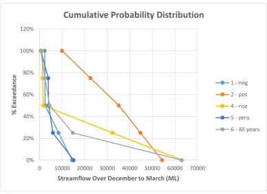
42 on the y-axis. Similarly in this analysis, the x-axis contained the streamflow total from the best particular season and the y-axis contained a percentage exceedance or probability scale from 0% to 100%. The graph contained six different probability lines consisting of the five SOI phases shown above and a sixth line which combines all five SOI phases into one. These six different SOI phases depicted the percentage chance that when the SOI is a certain phase, the total streamflow will be a certain amount within a certain season.

3.5 Combined Water Balance Model with ENSO Relationships

Once a definitive relationship was formed between streamflow and SOI, its findings were applied to the water balance model to create a water allocation tool that can be used to explore water management scenarios. Depending on the best seasonal relationship, a water balance model was run for the best seasonal time each year from 1965 to 1981 with fifteen seasons in total. Out of these fifteen seasons, there was a certain amount seasons that fall under each of the SOI phases according to the best lag increase. Therefore the end result from running 15 different water balance models gave a certain total storage volume held within Cressbrook Dam. To see whether certain SOI phases resulted in the total storage volume being higher or lower, a cumulative probably distribution similar to the process explained in the section above was used. In this case, the y-axis will still be a probability of exceedance from 0% to 100% but the x-axis showed the different end level storage volumes of Cressbrook Dam.

(57)

43 - A starting volume of 90% (73657.8 ML)

- A starting volume of 75% (61381.5 ML) - A starting volume of 50% (40921 ML) - A starting volume of 25% (20460.5 ML)

3.6 Scenarios

Once water allocation graphs were established for a range of starting volumes, it was important that their validities were investigated by exploring a range of alternative water management approaches based on their findings. To examine how the behaviour of Cressbrook Dam would have occurred by incorporating climate indices into decision-making, three different scenarios were run based on past historical streamflows. These three different scenarios were:

1. Normal water restrictions that are currently used by the TRC

2. Restrictions raised to level 2 from December to March when the SOI phase is observed to be consistently positive

3. Restrictions raised by one level from December to March when the SOI phase is observed to be consistently positive

3.6.1 Scenario 1

(58)

44 Table 5: Water Restrictions in Place by TRC

Restriction

Level 2 (Permanent Conservation)

Level 3 Level 4 Level 5

Useable Storage trigger point

to introduce restrictions

100% to 40% <40% <30% <20%

Useable storage trigger point

to lift restrictions

50% to 100% >50% >40% >30%

Water Consumption

(L/p/d)

250 210 170 125

An important note to take away from Table 4 is the use of ‘useable storage’. The useable storage is the different from using the maximum storage of the dam from 0 to 81842 ML and is calculated using the following equation:

𝑈𝑠𝑒𝑎𝑏𝑙𝑒 𝑆𝑡𝑜𝑟𝑎𝑔𝑒 (𝑀𝐿) = ((𝑇𝑜𝑡𝑎𝑙 𝑑𝑎𝑚 𝑠𝑡𝑜𝑟𝑎𝑔𝑒 – 𝑑𝑒𝑎𝑑 𝑠𝑡𝑜𝑟𝑎𝑔𝑒)

× 𝑃𝑒𝑟𝑐𝑒𝑛𝑡𝑎𝑔𝑒 𝑜𝑓 𝐷𝑎𝑚 𝐿𝑒𝑣𝑒𝑙 𝐹𝑢𝑙𝑙) + 𝑑𝑒𝑎𝑑 𝑠𝑡𝑜𝑟𝑎𝑔𝑒

Where

Total dam storage = 81842 ML And Dead storage = 2995 ML

(59)

45 3.6.2 Scenario 2

Scenario 2 incorporates a new layer of decision-making processes, with this layer being the current SOI phase. As seen in Figure 13 below, if the SOI phase in November was viewed to be 2 (consistently positive) and the current water restriction was not level 2, then the model will raise the restrictions straight to level 2 for the period of December to March.

(60)

46 3.6.3 Scenario 3

The last scenario analyses the behaviour of Cressbrook Dam using a more conservative approach than scenario 2 but has still taken SOI into consideration. The decision-tree shown in Figure 14 shows that this approach has raised the water level restrictions by one level instead of straight to level 2, when the SOI was observed to be phase 2 in November.

(61)

47 3.6.4 Development of Streamflows for Scenarios

The establishment of relationships between SOI and streamflow for the best months throughout the year and the best forecasting period were made from streamflow records that actually existed at the dam site itself. However when this record of 16 years of streamflow data were used to run the three various scenarios, the final result showed the storage level volume of the dam remained relatively high meaning that there was no difference between the different scenarios.

Therefore in order to make a comparable difference between the different scenarios other closed or open stream gauges that recorded flow from Cressbrook Creek were investigated. From the DNRM water monitoring panel, there are two other stream gauges that are found to record streamflow for Cressbrook Creek:

1) Cressbrook Creek at Tinton (downstream) – Available streamflow record from 1/10/1952 to 15/6/1986

2) Cressbrook Creek at Rosentretters Crossing (further downstream) – Available record from 20/8/1986 to now

(62)

48 To compare the error between the two datasets, the simulated and actual dam site streamflows from the four years were summed so that a comparison could be made between the cumulative volumes of each dataset. Once the relative error between the two was less than 5%, then these streamflows were used to simulate streamflows from the dam site dating back to 1/10/1952.

(63)

49

CHAPTER 4

RESULTS FOR STATISTICAL

STREAMFLOW FORECAST MODEL

4.1 Introduction

This chapter contains an in depth analysis of the results found from the relationship between ENSO and streamflow for Cressbrook Dam on a monthly and seasonal scale. From these relationships, cumulative probability distribution graphs for streamflows and storage levels were developed and discussed in detail.

4.2 Monthly Streamflow and ENSO Analysis

An assessment of the relationship between monthly SOI values and monthly streamflow totals for each month throughout the streamflow record were analysed. The resultant graphs from each of these months can be found in Appendix C which shows the r-squared values from zero month to a five month lag increase. To summarise the findings from these monthly SOI and streamflow relationship graphs, Table 6 below shows the average r-squared correlation for each month.

Table 6: Average Correlation Values for Each Month

Month R-Squared Value

January 0.277

February 0.209

March 0.271

April 0.0332

May 0.194

June 0.0530

July 0.0222

August 0.0349

September 0.0520

October 0.0623

November 0.00613

(64)

50 From these results, average r-squared values for every month were not anywhere close to approaching a value of 1 which indicates a perfect linear relationship between. Automatically, months that had a correlation of less than 0.1 were discarded and were not further investigated as a relationship this low cannot be used as a justification for future predictions. However, there were certain months which showed a significant enough relationship to investigate further. The months of December, January, February, March and May all had correlation values above 0.1. A reasonable explanation as to why certain months had a better correlation than other months is shown by Table 7 below which shows the total monthly streamflow that occurred for each month throughout the streamflow record.

Table 7: Monthly Streamflow Totals

Month Monthly Streamflow Total (ML/Month)

January 85076.75

February 94442.85

March 40668.01

April 14068.61

May 8059.1

June 36609.4

July 14966.67

August 9001.58

September 9037.72

October 9298.44

November 14082.82

(65)

51 If the streamflow totals are compared with the correlation values for each month respectively, then it is seen that there is trend where the best correlated months are associated with the highest streamflow totals. The months of January, February and March have the three highest streamflow totals and also have correlations above 0.1. The month of May was viewed to be an anomaly in the data as it had a high correlation for a small streamflow total. The months above and below May were viewed to be have little to no correlation and therefore was why May was also removed as a month to further investigate.

4.3 Seasonal Streamflow and ENSO Analysis

The best correlated months of December, January, February and March were added together to give a seasonal streamflow total for each year within the streamflow dataset. These streamflows where then assessed for their correlation against monthly SOI values with increasing one month lags, the same analysis used previously. Whereas the monthly relationships helped to identify the best timeframe to make streamflow predictions based off SOI, the seasonal relationship was used to identify the forecasting period.

Figure 15: Seasonal Streamflow and SOI Relationships R² = 0.5831

R² = 0.646

R² = 0.3672 R² = 0.431

R² = 0.4389

-20000 -10000 0 10000 20000 30000 40000 50000 60000 70000

-30 -20 -10 0 10 20 30 40

To ta l Se aso n al Str e am fl o w (M L/ se aso n ) SOI

December-March

(66)

52 Immediately from figure 15, the change in temporal scales from monthly to seasonal has resulted in correlations that are much higher than the monthly correlations. The lowest correlation is seen to be 0.431 for a lag of three months between streamflow and the SOI value observed in September. This correlation is higher than any average monthly r-squared value shown in Table 6 which coincides with the document produced by Klingaman (2012), which indicates that the effects ENSO are based on a seasonal to inter-annual temporal scale more so than a monthly temporal scale. The highest correlation between SOI and seasonal streamflow was for a one month lag period between the datasets with a value of 0.646. This indicates that the best forecasting period for the months of December to March are based on the SOI values that are observed in the month of November.