Spatial modelling of
Calanus finmarchicus
and
Calanus helgolandicus
: parameter
differences explain differences in
biogeography
Robert J. Wilson1,∗, Michael R. Heath1 and Douglas C. Speirs1
1Department of Mathematics and Statistics, University of Strathclyde, Glasgow,
Scotland
Correspondence*: Robert Wilson
Department of Mathematics and Statistics, University of Strathclyde, Glasgow, Scotland, [email protected]
ABSTRACT
2
The North Atlantic copepods Calanus finmarchicus and C. helgolandicus are moving north 3
in response to rising temperatures. Understanding the drivers of their relative geographic 4
distributions is required in order to anticipate future changes. To explore this, we created a 5
new spatially explicit stage-structured model of their populations throughout the North Atlantic. 6
Recent advances in understandingCalanusbiology, including U-shaped relationships between 7
growth and fecundity and temperature, and a new model of diapause duration are incorporated in 8
the model. Equations were identical for both species, but some parameters were species-specific. 9
The model was parameterized using Continuous Plankton Recorder Survey data and tested 10
using time series of abundance and fecundity. The geographic distributions of both species 11
were reproduced by assuming that only known interspecific differences and a difference in the 12
temperature influence on mortality exist. We show that differences in diapause capability are not 13
necessary to explain whyC. helgolandicusis restricted to the continental shelf. Smaller body size 14
and higher overwinter temperatures likely make true diapause implausible forC. helgolandicus. 15
Known differences were incapable of explaining why onlyC. helgolandicusexists southwest of 16
the British Isles. Further, the fecundity ofC. helgolandicus in the English Channel is much lower 17
than we predict. We hypothesize that food quality is a key influence on the population dynamics 18
of these species. The modelling framework presented can potentially be extended to further 19
Calanusspecies. 20
Keywords: copepods1, zooplankton2, modelling3, biogeography4, diapause5 21
Word count: 8,991. 22
1
INTRODUCTION
Zooplankton communities are now reorganizing throughout the North Atlantic (Chust et al., 2013; 23
their distribution, while they are retreating at the southern edge (Beaugrand, 2012). As a consequence, 25
communities are changing and many species are being replaced by their southern congenerics (Beaugrand 26
et al., 2002). 27
Changes in communities dominated by the calanoid copepodsCalanus finmarchicusandC. helgolandicus
28
are among the most well-studied (Wilson et al., 2015).C. finmarchicusis an oceanic species that is found 29
from the Gulf of Maine to the North Sea (Melle et al., 2014). In contrast,C. helgolandicusis a shelf species 30
that lives from the North Sea to the Mediterranean Sea (Bonnet et al., 2005). Both species are now moving 31
north, which has causedC. helgolandicusto replaceC. finmarchicusas the dominant calanoid copepod 32
in the North Sea (Reid et al., 2003). Future temperature rises will likely cause this to be repeated further 33
north (Villarino et al., 2015). We must therefore understand differences in the impacts of climate change on 34
congeneric zooplankton species, so that we can anticipate changes in communities and their consequences. 35
A key test of our understanding of the interspecific differences in demography of these species is whether 36
we can simulate their population dynamics in such a way that the relative geographic distributions of both 37
species are a result of the differences in biology. An inability to do this can highlight important knowledge 38
gaps that must be filled to make projections of the impact of climate change onCalanuscommunities more 39
biologically credible. 40
In this spirit, we tested the ability of known interspecific differences to explain the geographic distributions 41
of both species by creating a new unified model. We created a stage-structured model which represents 42
each life stage ofC. finmarchicusandC. helgolandicus, and that represents body size by dividing each 43
stage into a set of size classes. This work is based on the previous model ofC. finmarchicusin the North 44
Atlantic of Speirs et al. (2005, 2006). Continuous Plankton Recorder survey data was used to parameterize 45
the model and simulated annual cycles of abundance and fecundity were compared with empirical time 46
series in a number of North Atlantic locations. 47
Recently, an increasing number of researchers have taken a trait-based approach to understanding 48
zooplankton communities (Litchman et al., 2013; Barton et al., 2013). Key traits such as body size, 49
development rate and fecundity are identified, and the functional role of species in ecosystems is thus 50
thought to be a function of their positions within trait-space. A trait-based approach has previously been 51
used to model copepod communities in Cape Cod Bay, Massachussetts (Record et al., 2010). We used this 52
approach to understand the biogeography of two species, under the assumption that where species lie in 53
trait-space is the fundamental determinant of relative biogeography. 54
Our underlying philosophy is that the equations describing the population dynamics of both species 55
should be identical, but with potential differences in parameters. This constraint will arguably result 56
in suboptimal models for each species when viewed separately. However, it enables us to more clearly 57
understand the biological differences that drive the large-scale differences in distribution. Fundamentally, 58
this work is based on the assumption that if knowledge of key interspecific differences is sufficient, then 59
known interspecific differences are all that is needed for a model to reproduce the geographic distributions 60
of both species. The only known difference between the species that could influence population dynamics 61
is the response of ingestion rate, and thus growth, development and fecundity, to temperature (Wilson et al., 62
2015). We therefore begin with the hypothesis that this difference alone can explain most of the differences 63
2
MODEL
2.1 Model background and framework
65
We present an extension of the previous work by Speirs et al. (2005, 2006), who modelled the population 66
dynamics of C. finmarchicusover the entire North Atlantic. This extension took two key forms. First, 67
we incorporated recent developments in our understanding ofCalanusbiology. Second, we modified the 68
model of Speirs et al. (2006) so that it could represent the population dynamics of bothC. finmarchicus
69
andC. helgolandicus. Full mathematical details of the model, along with relevant parameters, are given in 70
Appendix 1. Here we will summarize the modelling framework of Speirs et al. and then the extensions to it. 71
The model of Speirs et al. was discrete in time and space. It covered the entire North Atlantic, ranging 72
from 30 to 80°N and 80°W to 90°E. The population ofC. finmarchicuswas distributed over a regular grid 73
of cells of size 0.5°longitude by 0.25°latitude. They had two update processes. First, the population of 74
each cell was updated to account for development, reproduction and mortality. After these updates, the 75
population is redistributed between cells to account for physical population transport. A separate physical 76
model was used to create the flow-field and temperature drivers for the relevant biological and physical 77
update. The annual cycle of food in each cell was estimated by deriving phytoplankton carbon fields from 78
satellite sea-colour observations. 1997 was used as the target year for simulations because this was the 79
year when the Trans-Atlantic Study ofCalanus (TASC) collected a large number of time series of C.
80
finmarchicusabundance in the North Atlantic. The framework of Speirs et al. was as follows. Surface 81
developers are made up of eggs (E), naupliar stages (N1 to N6), and copepodite stages (C1 to C5). Finally, 82
there are diapausers (C5d) and adults (C6). 83
Calanusdevelopment follows the equiproportional rule, that is relative stage duration is independent 84
of temperature (Campbell et al., 2001). Development from egg to adult can therefore be divided into a 85
fixed number of steps, with each having identical time duration under identical environmental conditions 86
(Gurney et al., 2001). In total, there were 57 development steps, which cover the 13 stages ofCalanus
87
development. 88
This framework allows the entire population to be updated simultaneously, and for the entire population to 89
be simulated with high computational efficiency (Speirs et al., 2006). However, modelling the populations 90
ofC. finmarchicusandC. helgolandicusrequired one modification. 91
We began with the hypothesis that differences in the response of growth and development to temperature 92
are sufficient to explain the geographic distributions of both species. In other words, all equations and 93
parameters would be the same, except for those related to growth and development. This could not be 94
satisfactorily achieved in the original framework. Large-scale patterns of fecundity are not only the result 95
of the effects of environmental conditions, but also of body size. Further, the ability of animals to diapause 96
is strongly influenced by size (Wilson et al., 2016). We therefore incorporated body size into the framework. 97
Large-scale patterns of fecundity and diapause duration could therefore be represented as the combined 98
effects of body size and the environment, and did not require the introduction of interspecific differences. 99
The geographic domain used by Speirs et al. covers all regions of highC. helgolandicusabundance (Bonnet 100
2.2 Biological processes: a new view ofCalanus biology
102
The following biological processes are represented in our model: development, egg production, diapause 103
and mortality. In each case, we modified the model of Speirs et al. to account for recent developments in 104
the understanding ofCalanusbiology. 105
A recent review of the differences between the two species found that the only known relevant difference 106
was the influence of temperature on ingestion, and thus growth, development and fecundity (Wilson et al., 107
2015). We therefore constrained the model by making a number of assumptions about the differences 108
between the species based on this review. These assumptions were as follows: 109
• There is a dome-shaped response of ingestion rate to temperature for both species, with 110
ingestion rate higher forC. finmarchicusthanC. helgolandicusbelow a temperature of 13 °C. 111
• An emergent property of this is that there are dome-shaped relationships between growth and 112
egg production rate and temperature, and a U-shaped relationship between development time 113
and temperature for both species. 114
• Under identical conditions, both species will grow to the same size. 115
• There are no differences in the ability to accumulate lipids or diapause. 116
Further, we take the following assumptions and simplifications about the biology and ecology of both 117
species. 118
• There are no interactions between the two species. 119
• The species do not hybridize. However, hybridization has been observed among otherCalanus
120
species (Gabrielsen et al., 2012; Parent et al., 2011, 2012). 121
• The relationships between traits and the environment do not vary in time or space. 122
The key modelled relationships between body size, development time, egg production rate and diapause 123
duration with temperature are shown in Fig. 1. 124
There are no apparent interspecific differences in body size, and large-scale geographic patterns of body 125
size are largely driven by temperature (Wilson et al., 2015). We therefore modeled body size under the 126
simplified assumption that it is determined by temperature experienced at birth for all development classes 127
(Fig. 1(a)). This assumption is derived from the fact that egg size is determined by temperature (Campbell 128
et al., 2001) and that the existence of an exo-skeleton likely greatly constrains size over all development 129
classes. The temperature-prosome length relationship of Campbell et al. (2001) was used with a multiplier, 130
which was fitted based on the relationship between predicted and observed female prosome length. Prosome 131
length reduces linearly with increasing temperature. This approach contrasts with Speirs et al., which did 132
not represent size. 133
Egg-adult development time was assumed to be influenced purely by temperature and food concentration. 134
The relationship between egg-adult development time and temperature under food-saturated conditions is 135
assumed to follow that derived by the model of Wilson et al. (2015). Development time saturates at high 136
food levels, and we use the relationship between food concentration and development time of Campbell 137
et al. (2001). There is a U-shaped response of development time to temperature (Fig. 1(b)), which contrasts 138
with the monotonically decreasing form used by Speirs et al. The computational approach is that of Gurney 139
2006) and it is effective in minimizing numerical diffusion (Gurney et al., 2001; Record and Pershing, 141
2008). 142
Fecundity was related to temperature, food concentration and body size. We assumed that egg production 143
and growth are equivalent (McLaren and Leonard, 1995). Egg laying females have stopped growing and 144
we therefore assume that carbon previously directed to growth will be used to make eggs. The growth rate 145
equation of Wilson et al. (2015) forms the basis of our egg production rate (EPR) model for both species, 146
with the food saturation component taken from Hirche et al. (1997). EPR therefore has a dome-shaped 147
response to temperature (Fig. 1(c)). Further, EPR has a saturating response to food concentration and we use 148
a conventional allometric relationship between EPR and carbon weight, i.e. EPR∼carbon weight0.75. This 149
contrasts with Speirs et al., who represented EPR as a monotonically increasing function of temperature, 150
but using the same food response as we have assumed. We assume that 50% of adults are female. 151
A recent modelling study, which synthesized empirical findings, showed that maximum potential diapause 152
duration is largely determined by prosome length and overwintering temperature (Wilson et al., 2016). 153
We therefore modelled diapause duration using the maximum potential diapause duration equation from 154
that study (Fig. 1(d)). Diapause duration declines at higher temperature because of increased metabolic 155
rates, and is shorter at smaller prosome lengths because of lower relative lipid levels and higher relative 156
metabolic costs. We assumed that a fraction of the C5 population enters diapause at the end of the C5 stage. 157
This fraction is dependent on growth rate, with it increasing at lower growth rates, so that more animals 158
diapause when development conditions are poor. In the model, animals exit diapause at the end of their 159
potential diapause duration. This differs from Speirs et al., who assumed that diapause exit was triggered 160
by a photoperiod cue. 161
Mortality is modelled using a stage-dependent background rate, alongside a starvation and density 162
dependent term. Field studies indicate that mortality in both species is stage-dependent (Eiane et al., 2002; 163
Ohman et al., 2004; Hirst et al., 2007). These estimates of stage-dependent mortality include all sources of 164
mortality. However, we need to distinguish between different sources of mortality to properly represent 165
population dynamics. We therefore used a fraction of the stage-specific mortality rates calculated by Eiane 166
et al. (2002) as the background mortality rate, with additional temperature, starvation and density dependent 167
terms. Starvation dependent mortality was modelled in the same way for both species by assuming that it 168
relates to growth rate; with starvation mortality only occurring below a threshold growth rate and increasing 169
as growth rate decreases. Background mortality is temperature dependent, with mortality increasing with 170
temperature and the relationship taking the form mortality ∼ (T /8)z. Density dependent mortality is 171
assumed to be proportional to total biomass. Mortality was represented the same way as in Speirs et al., 172
with the exception of starvation-dependence. Speirs et al. represented this purely as a function of food 173
concentration. However, the differences in ingestion rate between the two species (Møller et al., 2012) show 174
thatC. helgolandicusis likely to face much greater starvation levels at temperatures below approximately 175
11 °C. We therefore viewed growth rate as a better indicator of starvation than food concentration. 176
2.3 Environmental drivers
177
Seasonal cycles in food concentration, temperature and oceanic circulation drive the model. The only data 178
with sufficient spatial and temporal coverage of food concentration are satellite estimates of sea surface 179
colour. SeaWIFS satellite estimates of chlorophyll were therefore used to derive food fields. 180
Insufficient observations are available for 1997. We therefore used a climatological 8 day mean of 181
chlorophyll concentration from 1998-2000. There is a poor relationship between time series derived from 182
of Clarke et al. (2006), who developed a statistical methodology, where thin plate regression splines 184
modelled local estimates of chlorophyll concentration in relation to SeaWIFS estimates, bathymetry and 185
time of year. Field estimates of chlorophyll concentration in the top 5 m were used, assuming they reflect 186
chlorophyll concentration throughout the vertical distribution ofCalanus. However, it is possible that this 187
does not fully capture deep-water chlorophyll concentrations. Phytoplankton abundance was calculated 188
assuming that 1 mg m−3of Chlais equivalent to 40 mg Cm−3 (the approximate median of the values 189
reported by Parsons et al. (1984). Estimates of food extend to regions covered by sea ice, where we masked 190
food levels to zero. This mask was derived from 1997 satellite percentage ice cover from the Defence 191
Meteorological Satellite Program’s (DMSP) spatial sensor microwave/imager (SSM/I) (Comiso, 1997). 192
The approach taken to food was the same as in Speirs et al. 193
Temperature and velocity fields come from the Nucleus for European Modelling of the Ocean (NEMO) 194
Ocean General Circulation Model (OCGM) (version 3.2) (Madec, 2012). The forcings and model 195
implementation are described in Yool et al. (2011). NEMO is resolved at 64 vertical levels, and it 196
resolves the primitive equations on a C-type Arawkawa grid. Ocean surface forcing comes from the DFS4.1 197
fields produced by the European DRAKKAR collaboration. This differs from Speirs et al., who used the 198
OCCAM model to derive temperatures and flow fields. Computation of the NEMO model was performed 199
using the free Java tool Ichthyop version 3.2 (Lett et al., 2008). 200
We assumed that surface developers experience the temperatures and velocities which occur at a depth of 201
20 m. Diapause depth varies in space. We therefore derived a map of diapause from the data reported by 202
Heath et al. (2004). A loess smooth was used to estimate the median diapause depth in regions close to 203
where Heath et al. (2004) reported data. Where the smoothed estimate exceeded bathymetry, we used a 204
depth 10 metres shallower than the bathymetry at a location. In other regions we assumed that if bathymetry 205
was greater than 800 m that diapause depth was 800 m. For locations where bathymetry was shallower 206
than 800 m we used the predictions of a general additive model which related median diapause depth with 207
bathymetry using the data of Heath et al. (2004). Transport updates occurred every seven days. At the start 208
of each time step, 100 seeds were placed at the centre of each model cell. Particle trajectories over a 7-day 209
period were then calculated, and transition matrices were calculated to show the proportion of particles 210
which move to each nearby cell. The approach outlined above was in agreement with Speirs et al. 211
2.4 Data sources
212
The Continuous Plankton Recorder Survey 213
The Continuous Plankton Recorder Survey (CPR) is made up of data collected by devices attached to 214
ships which traverse commercial shipping lanes. It is designed for towing depths of 10 m at the operating 215
speeds of vessels (Batten et al., 2003). Water enters the CPR through a 1.27 cm2opening and is filtered by 216
a 270µm silk mesh. Abundance estimates are semi-quantitative, with each observation being placed in 217
one of 12 distinct abundance categories (Rae, 1952). CPR provides reliable temporal and spatial measures 218
(Batten et al., 2003; H´elaou¨et et al., 2016) of abundance. We used CPR data from 1958-2002. 219
Time series 220
The EU TASC project collected time series ofC. finmarchicuscopepodite abundance in 1997 at three 221
locations (Planque and Batten, 2000). Data was collected at Ocean Weather Ship Mike (OWS M) (66°N, 222
2°E) from 24 February to 17 December 1997 (Heath et al., 2000; Hirche et al., 2001) using a 180µm 223
mesh opening and closing multinet. Concentrations of copepodite stages (m−3) were converted to stage 224
the deep layer. We assume that deep animals were diapausing at that time. Per-capita egg production rates 226
were also recorded at this station (Niehoff et al., 1999). 227
Data was collected at 2 locations near the Westmann Islands (63°27.25’N, 20°00.00’W, depth 100 m, 228
and 63°22.20’N, 19°54.85’W, depth 200 m) (Gislason and Astthorsson, 2000). This site was visited 29 229
times, withC. finmarchicusbeing collected by vertically integrating hauls from 5 m above the seabed to the 230
surface with a 200µm mesh, 56 cm Bongo net. In addition, data was collected from Murchison (61°30.00’ 231
N, 01°40.00’ E, depth 160 m) on 29 occasions, using a 200µm mesh with a 30 cm Bongo net from a depth 232
of 150 m to the surface. 233
We include data from Ocean Weather Ship India (OWS I) (59°N, 19°E), which was collected between 234
1971 and 1975 (Irigoien, 1999). This time series is used because we lack data for a truly oceanic location 235
in 1997. Sampling occurred at approximately weekly intervals from 1971 to 1975 using oblique hauls of a 236
Longhurst-Hardy plankton recorder (280µm mesh). Stage-resolved copepod samples were then collected 237
from a depth of 500 m to the surface, with a resolution of 10 m. We used data from the top 100 m. 238
The US GLOBEC program started in 1995 (Durbin et al., 2000), and includes extensive zooplankton 239
sampling in the Gulf of Maine and Georges Bank.C. finmarchicusdensities (m−3) were estimated during 240
the first half of the year at varying depths using a 1 m2MOCNESS fitted with 0.15 mm mesh nets. Estimates 241
of density (m−2) were calculated for the top 100 m and from 100 m to the sea floor by considering regions 242
where bathymetry exceeded 200 m. 243
C. helgolandicusabundance data has been collected of Stonehaven, Scotland (56°57.8’ N, 2°6.2’W) since 244
1997. Sampling uses fine mesh nets, which collect an integrated sample of zooplankton throughout the 245
water column (Bresnan et al., 2015). Integrated abundance data is provided for C5, female and male stages. 246
Station L4 in the English Channel (50°15’N, 4°13’W) is one of the longest standing zooplankton time 247
series in European waters (Harris, 2010), with monitoring beginning in 1988. Seabed depth is 51 m, while 248
observations typically range between 40 and 45 times each year (Harris, 2010). This time series contains 249
information on the abundance of male, female and total copepodites, and egg production rate (Irigoien 250
et al., 2000). 251
2.5 Parameter derivation and sensitivity experiments
252
Our underlying goal was to reproduce the biogeography of both species displayed by the CPR. We 253
therefore carried out an extensive set of simulations to assess how well different parameter sets could 254
reproduce the geographic distributions of both species. 255
As discussed in section 2.2, laboratory and field data were used to derive the following traits: development 256
time, growth, fecundity, diapause duration, background mortality and body size. The remaining free, i.e. 257
unknown, parameters related to the equations for diapause entry and starvation and biomass dependent 258
mortality. We initially sought a single parameter set for mortality and diapause entry that would result in 259
credible predictions of geographic distributions for both species. However, a large number of exploratory 260
runs showed that this was not possible. We therefore sought parameter sets that reproduce the geographic 261
distributions of both species while minimizing the differences between the model parameters of both 262
species. A suite of runs showed that this was only achievable by assuming that mortality responded 263
differently to temperature in both species. 264
Model parameters were derived by simultaneously altering the terms for mortality and diapause entry for 265
into cells of dimension 2°E and 1°N, and we then removed cells without a CPR abundance record for each 267
month of the year. Annual mean abundance was then calculated by averaging the mean abundance of the 268
mean monthly abundance for C5 and adults in each cell. 269
This resulted in 333 cells for model comparisons. Each CPR abundance record represents approximately 270
3 m3 of filtered seawater (Richardson et al., 2006). Therefore, CPR data must be divided by 3 to get 271
estimates of abundance per m3. This must then be multiplied by a further conversion factor of 20 (Speirs 272
et al., 2006) to provide estimates of abundance (m−2) over the top 100 m of the water column. 273
Simulations began by seeding a large number of eggs over the entire North Atlantic and in the eastern 274
North Atlantic for C. finmarchicus and C. helgolandicus respectively. The model was then run to a 275
quasi-stable state and we then calculated the correlation coefficient (r) between predicted annual surface 276
abundance (m−2)) and CPR abundance (m−2)). 277
We report two sensitivity experiments. First, we show the geographic distributions of both species when 278
there are no interspecific differences in free parameters, i.e. only differences in growth, development 279
and fecundity are assumed. In this case we are using the diapause entry and starvation and temperature 280
dependent mortality parameters forC. helgolandicusfor both species. 281
Our initial model of diapause duration used a model of maximum potential diapause duration (Wilson 282
et al., 2016), which possibly results in diapause durations which are unrealistically long. We therefore 283
carried out a sensitivity analysis which relates the ability to reproduce the geographic distributions of 284
both species to the assumptions for diapause duration and temperature dependent mortality. Temperature 285
dependent mortality is proportional to (T /8)z for temperature T (°C). The parameterization assumed 286
different values ofzfor each species. 287
3
RESULTS
3.1 Model results
288
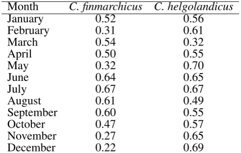
Fig. 2 and Fig. 3 compare the model predictions and CPR estimates of bimonthly abundance for C.
289
finmarchicusandC. helgolandicusrespectively. Table 1 shows the correlation coefficients between monthly 290
modelled and CPR abundance for both species. The large-scale geographic pattern ofC. finmarchicus
291
abundance was successfully reproduced in comparison with CPR. The correlation coefficient between 292
simulated mean annual abundance and CPR abundance over the 2°E by 1°N cells is 0.75. Bimonthly 293
comparisons betweenC. finmarchicuspredictions and the CPR abundance are shown in Fig. 2. Importantly, 294
we reproduced the relatively high abundance ofC. finmarchicusin the West Atlantic in autumn. In addition, 295
the model predicts a year round surface population in coastal waters in the West Atlantic, in accordance 296
with CPR. However, it perhaps over-predicted abundance in November and December. 297
A comparison of bimonthly predictions ofC. helgolandicusabundance with the CPR abundance is shown 298
in Fig. 3. The correlation coefficient between predicted mean annual abundance and CPR abundance over 299
the 2°E by 1°N cells was 0.76. Importantly,C. helgolandicuswas restricted to the continental shelf. The 300
autumn bloom ofC. helgolandicusin the North Sea was also reproduced. However, predicted abundance in 301
November and December in the region to the south west of the British Isles appears too high. 302
Fig. 4 shows simulated combined abundance for stage C5 and adultC. finmarchicuscompared with those 303
from the time series. Predicted peak abundances are within a factor of 2 of those recorded in the time series, 304
with the exception of the Westmann Islands. OWS I is notable for getting the scale of the first generation 305
failed to show the apparent sharp increase in C5 and adult at OWS M before day 100. Additionally, the 307
second peak in C5 and adult abundance at OWS M appears to be time shifted by approximately 50 d. 308
We compare predictions forC. helgolandicuswith field time series and time series derived from CPR 309
in Fig. 5. The timing of the autumn peak ofC. helgolandicusabundance at Stonehaven was successfully 310
reproduced. However, we failed to reproduce the small spring bloom. Predicted time and the magnitude of 311
peak abundance was close to that in the L4 time series. However, abundance appeared to be over-predicted 312
during winter. 313
Predicted EPR is compared with field time series at OWS M and L4 for C. finmarchicus and C.
314
helgolandicus respectively in Fig. 6. Predicted C. helgolandicusEPR is lower in the first half of the 315
year of the time series, and is slightly time shifted compared with the time series. Predictions depart 316
significantly from the times series in the second half of the year, with EPR being significantly higher than 317
in the time series. TheC. finmarchicusEPR time series at OWS M is of short duration. We can therefore 318
only make a limited comparison. However, the predicted EPR is approximately the same as the median 319
EPR in the time series. 320
3.2 Sensitivity experiments
321
In the results shown in section 3.1, the only differences between the species are the relationship between 322
growth, development and fecundity and temperature, and a parameterized difference in the response of 323
mortality to temperature. Fig. 7 shows the predicted geographic distribution ofC. finmarchicuswhen the 324
temperature-dependent mortality parameter forC. helgolandicuswas used. The geographic distribution in 325
the west Atlantic is successfully reproduced. However, the geographic distribution in the east Atlantic is 326
too southerly, with a large population predicted to exist in the Celtic Sea. 327
Exploratory simulations showed that the C. helgolandicus predictions were sensitive to diapause 328
assumptions. First, the model performed well ifC. helgolandicuswas assumed to remain at the surface 329
year round and to never diapause. In fact, this simplified model arguably performed better than the original. 330
The key features of the distribution of C. helgolandicuswere largely reproduced, with the correlation 331
coefficient (0.78) of model performance compared with CPR actually improving in comparison with our 332
original model. 333
Further exploratory simulations showed that the state of populations ofC. helgolandicusis sensitive to 334
diapause duration. A sensitivity analysis showed that small changes to diapause or mortality assumptions 335
can result in C. helgolandicus becoming an oceanic species. Fig. 8 shows the correlation coefficient 336
between predictions and CPR abundance of C. helgolandicusunder varying assumptions for diapause 337
duration and the scaling of mortality with temperature. A small reduction in how steeply mortality scales 338
with temperature results in a reduction in model performance, withC. helgolandicusbecoming an oceanic 339
species. Likewise, an increase in diapause duration can result inC. helgolandicusbecoming an oceanic 340
species. Notably, the high sensitivity to changes in temperature dependent mortality was not evident 341
diapause duration is reduced by 60%, which is potentially a more biologically realistic assumption for 342
diapause duration. 343
4
DISCUSSION
This study can be framed by a single question. What differences between C. finmarchicus and C.
344
helgolandicusexplain the relative geographic distributions of these two species? Alternatively, we can ask 345
In this setting, the model equations can be viewed as describing a genericCalanusspecies, while the 347
parameters determine where a species lies in trait space. We showed that the geographic distributions of 348
both species can be reproduced by assuming only two interspecific differences. These were the temperature 349
response of mortality and the temperature influence on ingestion rate, which in turn influences growth, 350
development and fecundity. In other words, we can effectively turnC. finmarchicusintoC. helgolandicus
351
by modifying those two traits. This framework has the potential to be applied to a number ofCalanus
352
species, and represents a complimentary approach to that taken by others (e.g. Record et al. (2010, 2013); 353
Maps et al. (2012)). 354
A key assumption underlying almost all population models ofCalanusis that growth and egg production 355
rate increase monotonically with temperature. This is the second study after Maar et al. (2013) to assume 356
they do not. Instead, we use a dome-shaped relationship between growth and fecundity and temperature. 357
Similar responses have now been established for a number of zooplankton species (Halsband-Lenk et al., 358
2002; Holste and Peck, 2006; Holste et al., 2009; Rhyne et al., 2009; White and Roman, 1992; Koski and 359
Kuosa, 1999; Pasternak et al., 2013). 360
The relationships between fecundity and development time and temperature were derived from the 361
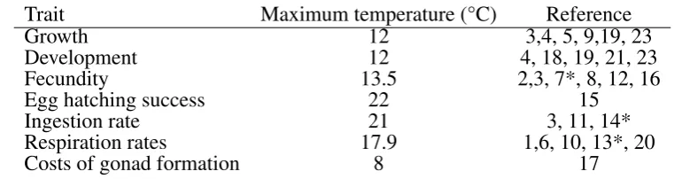
experimental ingestion rate data of Møller et al. (2012). A review of the literature shows that we have 362
little knowledge of the key traits ofC. finmarchicus such as development, growth and fecundity above 363
12 °C (Table 2). Further, we are not aware of published evidence of the influence of temperature onC.
364
helgolandicus’s fecundity. Clarifications of the relationship between growth and temperature are therefore 365
a priority ofCalanusresearch. Importantly, conventional models of development are problematic in the 366
context of climate change, where they may falsely predict ever increasing growth rates as temperatures rise. 367
This is highlighted in the Gulf of Maine, where despite summer surface temperatures now often exceeding 368
20 °C (Mills et al., 2013) there have recently been record high levels ofC. finmarchicusabundance (Runge 369
et al., 2014). 370
Understanding the relative geographic distributions of both species can arguably be answered by asking 371
why onlyC. helgolandicusexists in the region south west of the British Isles. On the basis of our models of 372
growth and fecundity, this region is not noticeably favourable toC. helgolandicus. However, the population 373
model’s performance is instructive. Simulated abundance ofC. helgolandicusis much higher in winter at 374
L4 than in reality, and we significantly over-predicted EPR in the second half of the year compared with 375
the long-term seasonal pattern (Maud et al., 2015). This is potentially related to food quality. Resolving the 376
apparent contradictions in understanding of the influence of food quality on fecundity (Maud et al., 2015; 377
Niehoff et al., 1999; Jønasdøttir et al., 2002) and development time (Diel and Klein Breteler, 1986) may 378
therefore be the key to fully explaining the relative biogeographies of both species. 379
Measuring mortality in copepods is commonly viewed as an intractable problem (Ohman, 2012), and 380
therefore models of mortality are inherently uncertain and difficult to validate. This problem is highlighted 381
by our formulation of starvation mortality, where it was related to growth rate. The formulation was 382
similar to that used by other modellers (e.g. Tittensor et al. (2003)), however it was ad-hoc and impossible 383
to validate. Importantly, the modelled biogeography ofC. helgolandicus was dependent on starvation 384
mortality, where it plays a key role in reducing post-diapause populations in oceanic regions to a low 385
enough level to eliminate long-term persistence. However, alternative formulations of mortality could 386
potentially achieve this. Some zooplankton modellers have used U-shaped relationships between mortality 387
and temperature (Rajakaruna et al., 2012), which could act as a limit on the north-western distribution 388
of C. helgolandicus. Further, allee effects (Kiørboe, 2006) and the impact of starvation on long-term 389
fecundity (Niehoff, 2004) could significantly deplete the populations of low-abundance post-diapauseC.
helgolandicuspopulations. Including these mortality effects in our model would result in a more complete 391
representation of copepod ecology. However, there is little evidence to quantify the relative magnitude of 392
these sources of mortality. Further advances in understanding copepod mortality (Gentleman et al., 2012; 393
Ohman, 2012) are therefore likely necessary to justify increasingly complex mortality models. However, 394
the influence of mortality should be considered if the model is to be applied, particularly in climate change 395
contexts where changes might be dependent on the specific mortality formulation. 396
There is a spring bloom ofC. helgolandicusin the North Sea (Bresnan et al., 2015), which we did not 397
predict. However, the apparent phenology ofC. helgolandicusin the North Sea is difficult to reconcile 398
with the known influence of temperature on its development time (Cook et al., 2007; Bonnet et al., 2009). 399
The first Stonehaven bloom typically occurs before day 130, and temperatures are below 9 °C before then. 400
Evidence indicates thatC. finmarchicuseither cannot develop from egg to adult (Bonnet et al., 2009) or has 401
a development time greater than 120 d at these temperatures (Møller et al., 2012). Research is therefore 402
needed to reconcile development time studies ofC. helgolandicusand phenology in the North Sea. Further, 403
additional model runs (not shown) indicated that most of the modelled autumn bloom in the northern 404
North Sea resulted from animals that are advected into the North Sea from the North. The importance of 405
advection for North SeaC. finmarchicuspopulations has been previously been studied (Heath et al., 1999), 406
however the role of advection in influencing year to year North SeaC. helgolandicusabundance has not. 407
It may be possible thatC. helgolandicusphenology in the North Sea can be explained by the existence 408
of hybrids of C. helgolandicus andC. finmarchicus. This is a speculative hypothesis. However, at the 409
fringes of its northern distribution,C. finmarchicushybridizes withC. glacialis(Berchenko and Stupnikova, 410
2014; Parent et al., 2011; Gabrielsen et al., 2012), and we cannot rule out a similar phenomenon forC.
411
finmarchicusandC. helgolandicus. 412
Finally, our model highlights the importance of lipid dynamics and deep-water temperatures as influences 413
on the distribution of Calanus. Existing statistical models of Calanus biogeography (Helaou¨et and 414
Beaugrand, 2007; Chust et al., 2013; Hinder et al., 2013) and projections of future distributions (Reygondeau 415
and Beaugrand, 2011; Villarino et al., 2015) have only considered surface conditions. However, the 416
distribution ofC. helgolandicusappears to be strongly influenced by deep-water temperatures. Conditions 417
in large parts of the North Atlantic are sufficient to support at least one generation ofC. helgolandicus, 418
but high overwintering temperatures result in the inability of a sufficiently large overwintering population 419
to maintain a persistent population. Recent work showed that projected potential diapause duration ofC.
420
finmarchicusin the Norwegian Sea under a high emissions scenario was largely unchanged this century, 421
whereas surface temperature increases significantly (Wilson et al., 2016). Development conditions will 422
therefore improve significantly forC. helgolandicusin the Norwegian Sea, whereas diapause conditions 423
would remain largely unchanged. There is therefore potential forC. helgolandicusto become an oceanic 424
species as a result of deep-water warming lagging that at the surface. Similarly, these marginal changes in 425
potential diapause duration may act as a brake on the northward retreat ofC. finmarchicus. However, the 426
expected temperature increases across the North Atlantic will reduce lipid levels of animals (Wilson et al., 427
2016) and the consequences are poorly understood. The future evolution of lipid dynamics may therefore 428
be pivotal in determining the fate ofCalanuscommunities and will have important consequences for the 429
fish, seabirds and marine mammals that depend on the lipids provided by copepods (Beaugrand and Kirby, 430
DISCLOSURE/CONFLICT-OF-INTEREST STATEMENT
The authors declare that the research was conducted in the absence of any commercial or financial 432
relationships that could be construed as a potential conflict of interest. 433
AUTHOR CONTRIBUTIONS
RJW, MRH and DCS contributed to the design of the model. RJW implemented and analyzed the model 434
and led the writing of the paper. All authors contributed to the editing and refining of the paper. 435
ACKNOWLEDGMENTS
We thank Neil Banas for fruitful discussions that helped shape the diapause model in the paper. Andrew 436
Yool provided output from the NEMO model. Nicholas Record and a second anonymous reviewer provided 437
helpful critical comments which improved the manuscript. Finally, we thank Ian Thurlbeck for invaluable 438
IT support. 439
Funding: This work received funding from the MASTS pooling initiative (The Marine Alliance for 440
Science and Technology for Scotland) and their support is gratefully acknowledged. MASTS is funded by 441
the Scottish Funding Council (grant reference HR09011) and contributing institutions. 442
REFERENCES
Barton, A. D., Pershing, A. J., Litchman, E., Record, N. R., Edwards, K. F., Finkel, Z. V., et al. (2013). 443
The biogeography of marine plankton traits. Ecology Letters16, 522–34. doi:10.1111/ele.12063 444
Batten, S. D., Clark, R., Flinkman, J., Hays, G., John, E., John, A. W. G., et al. (2003). CPR sampling: the 445
technical background, materials and methods, consistency and comparability. Progress in Oceanography
446
58, 193–215. doi:10.1016/j.pocean.2003.08.004 447
Beaugrand, G. (2012). Unanticipated biological changes and global warming. Marine Ecology Progress
448
Series445, 293–301. doi:10.3354/meps09493 449
Beaugrand, G. and Kirby, R. R. (2010). Climate, plankton and cod.Global Change Biology16, 1268–1280. 450
doi:10.1111/j.1365-2486.2009.02063.x 451
Beaugrand, G., Luczak, C., and Edwards, M. (2009). Rapid biogeographical plankton shifts in the North 452
Atlantic Ocean. Global Change Biology15, 1790–1803. doi:10.1111/j.1365-2486.2009.01848.x 453
Beaugrand, G., Reid, P. C., Iba˜nez, F., Lindley, J. A., and Edwards, M. (2002). Reorganization of North 454
Atlantic marine copepod biodiversity and climate. Science296, 1692–4. doi:10.1126/science.1071329 455
Berchenko, I. V. and Stupnikova, A. N. (2014). Morphological peculiarities of Calanus finmarchicus
456
andCalanus glacialisin the areas of the co-existence of their populations. Oceanology54, 450–457. 457
doi:10.1134/S0001437014040031 458
Bonnet, D., Harris, R. P., Yebra, L., Guilhaumon, F., Conway, D. V. P., and Hirst, A. G. (2009). Temperature 459
effects onCalanus helgolandicus(Copepoda: Calanoida) development time and egg production. Journal
460
of Plankton Research31, 31–44. doi:10.1093/plankt/fbn099 461
Bonnet, D., Richardson, A., Harris, R., Hirst, A., Beaugrand, G., Edwards, M., et al. (2005). An 462
overview ofCalanus helgolandicusecology in European waters. Progress In Oceanography65, 1–53. 463
Bresnan, E., Cook, K. B., Hughes, S. L., Hay, S. J., Smith, K., Walsham, P., et al. (2015). Seasonality of 465
the plankton community at an east and west coast monitoring site in Scottish waters. Journal of Sea
466
Researchdoi:10.1016/j.seares.2015.06.009 467
Campbell, R. G., Wagner, M. M., Teegarden, G. J., Boudreau, C. A., and Durbin, E. G. (2001). Growth 468
and development rates ofCalanus finmarchicusthe copepod reared in the laboratory. Marine Ecology
469
Progress Series221, 161–183. doi:10.3354/meps221161 470
Chust, G., Castellani, C., Licandro, P., Ibaibarriaga, L., Sagarminaga, Y., and Irigoien, X. (2013). Are 471
Calanusspp. shifting poleward in the North Atlantic? A habitat modelling approach. ICES Journal of
472
Marine Science71, 241–253. doi:10.1093/icesjms/fst147 473
Clarke, E. D., Speirs, D. C., Heath, M., Wood, S. N., Gurney, W. S. C., and Holmes, S. J. (2006). Calibrating 474
remotely sensed chlorophyll-a data by using penalized regression splines. Journal of the Royal Statistical
475
Society: Series C (Applied Statistics)55, 331–353. doi:10.1111/j.1467-9876.2006.00540.x 476
Comiso, J. (1997). Bootstrap Sea Ice Concentrations from Nimbus-7 SMMR and DMSP SSM/I-SSMIS
477
(Boulder: Natinoal Snow and Ice Data Center) 478
Cook, K. B., Bunker, A., Hay, S., Hirst, A. G., and Speirs, D. C. (2007). Naupliar development times 479
and survival of the copepodsCalanus helgolandicusandCalanus finmarchicusin relation to food and 480
temperature. Journal of Plankton Research29, 757–767. doi:10.1093/plankt/fbm056 481
Corkett, C. J., Mclaren, I. A., and Sevigny, J.-M. (1986). The rearing of the marine calanoid copepods 482
Calanus finmarchicus(Gunnerus),C. glacialisJaschnov andC. hyperboreusKrøyer with comment on 483
the equiproportional rule. Syllogeus58, 539–546 484
Diel, S. and Klein Breteler, W. C. M. (1986). Growth and development ofCalanusspp. (Copepoda) during 485
spring phytoplankton succession in the North Sea.Marine Biology92, 85–92. doi:10.1007/BF00397574 486
Durbin, E. G., Garrahan, P. R., and Casas, M. C. (2000). Abundance and distribution of Calanus
487
finmarchicuson the Georges Bank during 1995 and 1996.ICES Journal of Marine Science57, 1664–1685. 488
doi:10.1006/jmsc.2000.0974 489
Eiane, K., Aksnes, D. L., Ohman, M. D., Wood, S., and Martinussen, M. B. (2002). Stage-specific mortality 490
ofCalanusspp. under different predation regimes. Sarsia47, 636–645. doi:10.4319/lo.2002.47.3.0636 491
Frederiksen, M., Anker-Nilssen, T., Beaugrand, G., and Wanless, S. (2013). Climate, copepods and 492
seabirds in the boreal Northeast Atlantic - current state and future outlook. Global Change biology19, 493
364–72. doi:10.1111/gcb.12072 494
Gabrielsen, T. M., Merkel, B., Sreide, J. E., Johansson-Karlsson, E., Bailey, A., Vogedes, D., et al. (2012). 495
Potential misidentifications of two climate indicator species of the marine arctic ecosystem:Calanus
496
glacialisandC. finmarchicus. Polar Biology35, 1621–1628. doi:10.1007/s00300-012-1202-7 497
Gentleman, W. C., Pepin, P., and Doucette, S. (2012). Estimating mortality: Clarifying assumptions and 498
sources of uncertainty in vertical methods. Journal of Marine Systems105-108, 1–19. doi:10.1016/j. 499
jmarsys.2012.05.006 500
Gislason, A. and Astthorsson, O. S. (2000). Winter distribution, ontogenetic migration, and rates of 501
egg production ofCalanus finmarchicus southwest of Iceland. ICES Journal of Marine Science 57, 502
1727–1739. doi:10.1006/jmsc.2000.0951 503
Gurney, W. S. C., Speirs, D. C., Wood, S. N., Clarke, E. D., and Heath, M. R. (2001). Simulating spatially 504
and physiologically structured populations. Journal of Animal Ecology70, 881–894. doi:10.1046/j. 505
0021-8790.2001.00549.x 506
Halsband-Lenk, C., Hirche, H.-J., and Carlotti, F. (2002). Temperature impact on reproduction and 507
development of congener copepod populations. Journal of Experimental Marine Biology and Ecology
508
Harris, R. (2000). Feeding, growth, and reproduction in the genusCalanus. ICES Journal of Marine
510
Science57, 1708–1726. doi:10.1006/jmsc.2000.0959 511
Harris, R. (2010). The L4 time-series: the first 20 years. Journal of Plankton Research 32, 577–583. 512
doi:10.1093/plankt/fbq021 513
Heath, M. R., Astthorsson, O. S., Dunn, J., Ellertsen, B., Gaard, E., Gislason, A., et al. (2000). Comparative 514
analysis ofCalanus finmarchicusdemography at locations around the Northeast Atlantic. ICES Journal
515
of Marine Science57, 1562–1580. doi:10.1006/jmsc.2000.0950 516
Heath, M. R., Backhaus, J. O., Richardson, K., McKenzie, E., Slagstad, D., Beare, D., et al. (1999). Climate 517
fluctuations and the spring invasion of the North Sea byCalanus finmarchicus. Fisheries Oceanography
518
8, 163–176. doi:10.1046/j.1365-2419.1999.00008.x 519
Heath, M. R., Boyle, P., Gislason, A., Gurney, W. S. C., Hay, S. J., Head, E. J. H., et al. (2004). Comparative 520
ecology of over-winteringCalanus finmarchicus in the northern North Atlantic, and implications for 521
life-cycle patterns. ICES Journal of Marine Science61, 698–708. doi:10.1016/j.icesjms.2004.03.013 522
Helaou¨et, P. and Beaugrand, G. (2007). Macroecology ofCalanus finmarchicusandC. helgolandicusin 523
the North Atlantic Ocean and adjacent seas. Marine Ecology Progress Series345, 147–165. doi:10. 524
3354/meps06775 525
H´elaou¨et, P., Beaugrand, G., and Reygondeau, G. (2016). Reliability of spatial and temporal patterns of 526
C. finmarchicusinferred from the CPR survey. Journal of Marine Systems153, 18–24. doi:10.1016/j. 527
jmarsys.2015.09.001 528
Hinder, S. L., Gravenor, M. B., Edwards, M., Ostle, C., Bodger, O. G., Lee, P. L. M., et al. (2013). 529
Multi-decadal range changes vs. thermal adaptation for north east Atlantic oceanic copepods in the face 530
of climate change. Global Change Biology20, 140–146. doi:10.1111/gcb.12387 531
Hirche, H.-J. (1983). Overwintering ofCalanus finmarchicusandCalanus helgolandicus. Marine Ecology
532
Progress Series11, 281–290 533
Hirche, H.-J. (1987). Temperature and plankton II. Effect on respiration and swimming activity in copepods 534
from the Greenland Sea. Marine Biology95, 347–356. doi:10.1007/BF00428240 535
Hirche, H.-J., Brey, T., and Niehoff, B. (2001). A high-frequency time series at Ocean Weather Ship 536
Station M (Norwegian Sea): population dynamics ofCalanus finmarchicus. Marine Ecology Progress
537
Series219, 205–219. doi:10.3354/meps219205 538
Hirche, H.-J., Meyer, U., and Niehoff, B. (1997). Egg production ofCalanus finmarchicus: effect of 539
temperature, food and season. Marine Biology127, 609–620. doi:10.1007/s002270050051 540
Hirst, A. G., Bonnet, D., and Harris, R. P. (2007). Seasonal dynamics and mortality rates ofCalanus
541
helgolandicusover two years at a station in the English Channel. Marine Ecology Progress Series340, 542
189–205. doi:10.3354/meps340189 543
Holste, L. and Peck, M. A. (2006). The effects of temperature and salinity on egg production and hatching 544
success of BalticAcartia tonsa(Copepoda: Calanoida): a laboratory investigation. Marine Biology148, 545
1061–1070. doi:10.1007/s00227-005-0132-0 546
Holste, L., St. John, M. A., and Peck, M. A. (2009). The effects of temperature and salinity on reproductive 547
success of Temora longicornisin the Baltic Sea: a copepod coping with a tough situation. Marine
548
Biology156, 527–540. doi:10.1007/s00227-008-1101-1 549
Hygum, B. H., Rey, C., and Hansen, B. W. (2000a). Growth and development rates ofCalanus finmarchicus
550
nauplii during a diatom spring bloom. Marine Biology136, 1075–1085. doi:10.1007/s002270000313 551
Hygum, B. H., Rey, C., Hansen, B. W., and Tande, K. (2000b). Importance of food quantity to structural 552
growth rate and neutral lipid reserves accumulated in Calanus finmarchicus. Marine Biology 136, 553
Ikeda, T., Kanno, Y., Ozaki, K., and Shinada, A. (2001). Metabolic rates of epipelagic marine copepods as 555
a function of body mass and temperature. Marine Biology139, 587–596. doi:10.1007/s002270100608 556
Ingvarsdøttir, A., Houlihan, D. F., Heath, M. R., and Hay, S. J. (1999). Seasonal changes in respiration 557
rates of copepodite stage V Calanus finmarchicus (Gunnerus). Fisheries Oceanography 8, 73–83. 558
doi:10.1046/j.1365-2419.1999.00002.x 559
Irigoien, X. (1999). Vertical distribution and population structure ofCalanusfimarchicus at station India 560
(59 °N, 19 °W) during the passage of the great salinity anomaly , 1971-1975. Deep-Sea Research Part I
561
47, 1–26. doi:10.1016/S0967-0637(99)00045-X 562
Irigoien, X., Head, R. N., Harris, R. P., Cummings, D., and Harbour, D. (2000). Feeding selectivity and 563
egg production ofCalanus helgolandicusin the English Channel. Limnology and Oceanography45, 564
44–54. doi:10.4319/lo.2000.45.1.0044 565
Jønasdøttir, S. H., Gudfinnsson, H. G., Gislason, A., and Astthorsson, O. S. (2002). Diet composition and 566
quality forCalanus finmarchicusegg production and hatching success off south-west Iceland. Marine
567
Biology140, 1195–1206. doi:10.1007/s00227-002-0782-0 568
Kiørboe, T. (2006). Sex, sex-ratios, and the dynamics of pelagic copepod populations. Oecologia148, 569
40–50. doi:10.1007/s00442-005-0346-3 570
Kjellerup, S., D¨unweber, M., Swalethorp, R., Nielsen, T. G., Møller, E. F., Markager, S., et al. (2012). 571
Effects of a future warmer ocean on the coexisting copepodsCalanus finmarchicusandC. glacialisin 572
Disko Bay, western Greenland. Marine Ecology Progress Series447, 87–108. doi:10.3354/meps09551 573
Koski, M. and Kuosa, H. (1999). The effect of temperature, food concentration and female size on the egg 574
production of the planktonic copepodAcartia bifilosa. Journal of Plankton Research21, 1779–1789. 575
doi:10.1093/plankt/21.9.1779 576
Lett, C., Verley, P., Mullon, C., Parada, C., Brochier, T., Penven, P., et al. (2008). A Lagrangian 577
tool for modelling ichthyoplankton dynamics. Environmental Modelling & Software23, 1210–1214. 578
doi:10.1016/j.envsoft.2008.02.005 579
Litchman, E., Ohman, M. D., and Kiørboe, T. (2013). Trait-based approaches to zooplankton communities. 580
Journal of Plankton Research35, 473–484. doi:10.1093/plankt/fbt019 581
Lynch, D. R., Lewis, C. V. W., and Werner, F. E. (2001). Can Georges Bank larval cod survive on a 582
calanoid diet? Deep-Sea Research Part II 48, 609–630. doi:10.1016/S0967-0645(00)00129-6 583
Maar, M., Møller, E. F., G¨urkan, Z., Jønasdøttir, S. H., and Nielsen, T. G. (2013). Sensitivity ofCalanus
584
spp. copepods to environmental changes in the North Sea using life-stage structured models. Progress in
585
Oceanography111, 24–37. doi:10.1016/j.pocean.2012.10.004 586
Madec, G. (2012). NEMO ocean engine. Note du Pole de mod´elisation, Institut Pierre-Simon Laplace
587
(IPSL), France
588
Maps, F., Pershing, A. J., and Record, N. R. (2012). A generalized approach for simulating growth 589
and development in diverse marine copepod species. ICES Journal of Marine Science69, 370–379. 590
doi:10.1093/icesjms/fsr182 591
Maps, F., Record, N. R., and Pershing, A. J. (2014). A metabolic approach to dormancy in pelagic 592
copepods helps explaining inter- and intra-specific variability in life-history strategies. Journal of
593
Plankton Research36, 18–30. doi:10.1093/plankt/fbt100 594
Maud, J. L., Atkinson, A., Hirst, A. G., Lindeque, P. K., Widdicombe, C. E., Harmer, R. a., et al. (2015). 595
How does Calanus helgolandicus maintain its population in a variable environment? Analysis of a 596
25-year time series from the English Channel. Progress in Oceanography137, 513–523. doi:10.1016/j. 597
McLaren, I. A. and Leonard, A. (1995). Assessing the equivalence of growth and egg production of 599
copepods. ICES Journal of Marine Science52, 397–408. doi:10.1016/1054-3139(95)80055-7 600
Melle, W., Runge, J., Head, E., Plourde, S., Castellani, C., Licandro, P., et al. (2014). The North Atlantic 601
Ocean as habitat forCalanus finmarchicus: Environmental factors and life history traits. Progress in
602
Oceanography129, 244–284. doi:10.1016/j.pocean.2014.04.026 603
Meyer, B., Irigoien, X., Graeve, M., Head, R. N., and Harris, R. P. (2002). Feeding rates and selectivity 604
among nauplii, copepodites and adult females ofCalanus finmarchicus and Calanus helgolandicus. 605
Helgoland Marine Research56, 169–176. doi:10.1007/s10152-002-0105-3 606
Mills, K., Pershing, A., and Brown, C. (2013). Fisheries management in a changing climate: Lessons 607
from the 2012 ocean heat wave in the northwest Atlantic. Oceanography 26, 191–195. doi:http: 608
//dx.doi.org/10.5670/oceanog.2013.27 609
Møller, E. F., Maar, M., J´onasd´ottir, S. H., Gissel Nielsen, T., and T¨onnesson, K. (2012). The effect of 610
changes in temperature and food on the development ofCalanus finmarchicusandCalanus helgolandicus
611
populations. Limnology and Oceanography57, 211–220. doi:10.4319/lo.2012.57.1.0211 612
Niehoff, B. (2004). The effect of food limitation on gonad development and egg production of the 613
planktonic copepodCalanus finmarchicus. Journal of Experimental Marine Biology and Ecology307, 614
237–259. doi:10.1016/j.jembe.2004.02.006 615
Niehoff, B., Klenke, U., Hirche, H. J., Irigoien, X., Head, R., and Harris, R. (1999). A high frequency time 616
series at Weathership M, Norwegian Sea, during the 1997 spring bloom: the reproductive biology of 617
Calanus finmarchicus. Marine Ecology Progress Series176, 81–92. doi:10.3354/meps176081 618
Ohman, M. D. (2012). Estimation of mortality for stage-structured zooplankton populations: What is to be 619
done? Journal of Marine Systems93, 4–10. doi:10.1016/j.jmarsys.2011.05.008 620
Ohman, M. D., Eiane, K., Durbin, E. G., Runge, J. A., and Hirche, H. J. (2004). A comparative study of 621
Calanus finmarchicusmortality patterns at five localities in the North Atlantic. ICES Journal of Marine
622
Science61, 687–697. doi:10.1016/j.icesjms.2004.03.016 623
Parent, G. J., Plourde, S., and Turgeon, J. (2011). Overlapping size ranges ofCalanusspp. off the Canadian 624
Arctic and Atlantic Coasts: impact on species’ abundances. Journal of Plankton Research33, 1654–1665. 625
doi:10.1093/plankt/fbr072 626
Parent, G. J., Plourde, S., and Turgeon, J. (2012). Natural hybridization betweenCalanus finmarchicus
627
andC. glacialis(Copepoda) in the Arctic and Northwest Atlantic. Limnology and Oceanography57, 628
1057–1066. doi:10.4319/lo.2012.57.4.1057 629
Parsons, T. R., Takahashi, M., and Hargrave, B. (1984). Biological oceanographic processes(Oxford: 630
Pergamon Press) 631
Pasternak, A. F., Arashkevich, E. G., Grothe, U., Nikishina, A. B., and Solovyev, K. A. (2013). Different 632
effects of increased water temperature on egg production of Calanus finmarchicus and C. glacialis. 633
Marine Biology53, 547–553. doi:10.1134/S0001437013040085 634
Pepin, P. and Head, E. J. H. (2009). Seasonal and depth-dependent variations in the size and lipid contents 635
of stage 5 copepodites ofCalanus finmarchicusin the waters of the Newfoundland Shelf and the Labrador 636
Sea. Deep-Sea Research I 56, 989–1002. doi:10.1016/j.dsr.2009.01.005 637
Planque, B. and Batten, S. D. (2000). Calanus finmarchicusin the North Atlantic: the year ofCalanusin 638
the context of interdecadal change. ICES Journal of Marine Science: Journal du Conseil57, 1528–1535. 639
doi:10.1006/jmsc.2000.0970 640
Preziosi, B. M. and Runge, J. A. (2014). The effect of warm temperatures on hatching success of the 641
marine planktonic copepod, Calanus finmarchicus. Journal of Plankton Research 36, 1381–1384. 642
Rae, K. S. M. (1952). Continuous plankton records: explanation and methods, 1946-1949. Bulletins of
644
Marine Ecology3, 135–155 645
Rajakaruna, H., Strasser, C., and Lewis, M. (2012). Identifying non-invasible habitats for marine copepods 646
using temperature-dependent R 0. Biological Invasions14, 633–647. doi:10.1007/s10530-011-0104-x 647
Record, N. R. and Pershing, A. J. (2008). Modeling zooplankton development using the monotonic 648
upstream scheme for conservation laws. Limnology and Oceanography: Methods6, 364–373. doi:10. 649
4319/lom.2008.6.364 650
Record, N. R., Pershing, A. J., and Maps, F. (2013). Emergent copepod communities in an adaptive 651
trait-structured model. Ecological Modelling260, 11–24. doi:10.1016/j.ecolmodel.2013.03.018 652
Record, N. R., Pershing, A. J., Runge, J. A., Mayo, C. A., Monger, B. C., and Chen, C. (2010). Improving 653
ecological forecasts of copepod community dynamics using genetic algorithms. Journal of Marine
654
Systems82, 96–110. doi:10.1016/j.jmarsys.2010.04.001 655
Reid, P. C., Edwards, M., Beaugrand, G., Skogen, M., and Stevens, D. (2003). Periodic changes in 656
the zooplankton of the North Sea during the twentieth century linked to oceanic inflow. Fisheries
657
Oceanography12, 260–269. doi:10.1046/j.1365-2419.2003.00252.x 658
Rey, C., Carlotti, F., Tande, K., and Hansen, B. H. (1999). Egg and faecal pellet production ofCalanus
659
finmarchicusfemales from controlled mesocosms and in situ populations: influence of age and feeding 660
history. Marine Ecology Progress Series188, 133–148. doi:10.3354/meps188133 661
Rey-Rassat, C., Irigoien, X., Harris, R., and Carlotti, F. (2002). Energetic cost of gonad development in 662
Calanus finmarchicusand C. helgolandicus. Marine Ecology Progress Series 238, 301–306. doi:10. 663
3354/meps238301 664
Reygondeau, G. and Beaugrand, G. (2011). Future climate-driven shifts in distribution of Calanus
665
finmarchicus. Global Change Biology17, 756–766. doi:10.1111/j.1365-2486.2010.02310.x 666
Rhyne, A. L., Ohs, C. L., and Stenn, E. (2009). Effects of temperature on reproduction and survival of 667
the calanoid copepodPseudodiaptomus pelagicus. Aquaculture292, 53–59. doi:10.1016/j.aquaculture. 668
2009.03.041 669
Richardson, A. J., Walne, A. W., John, A. W. G., Jonas, T. D., Lindley, J. A., Sims, D. W., et al. (2006). 670
Using Continuous Plankton Recorder data. Progress in Oceanography68, 27–74. doi:10.1016/j.pocean. 671
2005.09.011 672
Runge, J. A., Ji, R., Thompson, C. R. S., Record, N. R., Chen, C., Vandemark, D. C., et al. (2014). 673
Persistence of Calanus finmarchicus in the western Gulf of Maine during recent extreme warming. 674
Journal of Plankton Research37, 221–232. doi:10.1093/plankt/fbu098 675
Runge, J. A. and Plourde, S. (1996). Fecundity characteristics ofCalanus finmarchicusin coastal waters of 676
eastern Canada. Ophelia44, 171–187. doi:10.1080/00785326.1995.10429846 677
Runge, J. A., Plourde, S., Joly, P., Niehoff, B., and Durbin, E. (2006). Characteristics of egg production of 678
the planktonic copepod,Calanus finmarchicus, on Georges Bank: 1994-1999. Deep-Sea Research Part
679
II 53, 2618–2631. doi:10.1016/j.dsr2.2006.08.010 680
Saumweber, W. J. and Durbin, E. G. (2006). Estimating potential diapause duration inCalanus finmarchicus. 681
Deep-Sea Research Part II 53, 2597–2617. doi:10.1016/j.dsr2.2006.08.003 682
Speirs, D. C., Gurney, W. S. C., Heath, M. R., Horbelt, W., Wood, S. N., and de Cuevas, B. A. (2006). 683
Ocean-scale modelling of the distribution, abundance, and seasonal dynamics of the copepodCalanus
684
finmarchicus. Marine Ecology Progress Series313, 173–192. doi:10.3354/meps313173 685
Speirs, D. C., Gurney, W. S. C., Heath, M. R., and Wood, S. N. (2005). Modelling the basin-scale 686
demography ofCalanus finmarchicusin the north-east Atlantic. Fisheries Oceanography14, 333–358. 687
Tande, K. S. (1988). Aspects of developmental and mortality rates inCalanus finmarchicusrelated to 689
equiproportional development. Marine Ecology Progress Series44, 51–58. doi:10.1155/2012/803637 690
Tittensor, D. P., Deyoung, B., and Tang, C. L. (2003). Modelling the distribution, sustainability and diapause 691
emergence timing of the copepodCalanus finmarchicusin the Labrador Sea. Fisheries Oceanography
692
12, 299–316 693
Villarino, E., Chust, G., Licandro, P., Butensch¨on, M., Ibaibarriaga, L., Larra˜naga, a., et al. (2015). 694
Modelling the future biogeography of North Atlantic zooplankton communities in response to climate 695
change. Marine Ecology Progress Series531, 121–142. doi:10.3354/meps11299 696
White, J. R. and Roman, M. R. (1992). Egg production by the calanoid copepodAcartia tonsain the 697
mesohaline Chesapeake Bay: the importance of food resources and temperature. Marine Ecology
698
Progress Series86, 239–249 699
Wilson, R. J., Banas, N. S., Heath, M. R., and Speirs, D. C. (2016). Projected impacts of 21st century climate 700
change on diapause inCalanus finmarchicus. Global Change Biology, 1–9doi:10.1111/gcb.13282 701
Wilson, R. J., Speirs, D. C., and Heath, M. R. (2015). On the surprising lack of differences between 702
two congeneric calanoid copepod species, Calanus finmarchicusand C. helgolandicus. Progress in
703
Oceanography134, 413–431. doi:10.1016/j.pocean.2014.12.008 704
Yool, A., Popova, E. E., and Anderson, T. R. (2011). Medusa-1.0: a new intermediate complexity 705
plankton ecosystem model for the global domain. Geoscientific Model Development 4, 381–417. 706
TABLE CAPTIONS
Table 1: The correlation coefficient (r) between modelled monthly abundance and the mean CPR abundance 708
in each cell. 709
Table 2: Temperature ranges for measurement of keyC. finmarchicustraits. * indicates the reference with 710
the highest report temperature. References: Ingvarsdøttir et al., 1999; 2. Rey et al., 1999; 3. Harris, 2000; 4. 711
Campbell et al., 2001 5. Hygum et al., 2000b; 6. Saumweber and Durbin, 2006; 7. Runge and Plourde, 712
1996; 10. Hirche, 1983; 11. Meyer et al., 2002; 12. Hirche et al., 1997; 13. Hirche, 1987; 14. Møller et al., 713
2012; 15. Preziosi and Runge, 2014; 16. Kjellerup et al., 2012; 17. Rey-Rassat et al., 2002; 18. Cook et al., 714
2007; 19. Hygum et al., 2000a; 20. Ikeda et al., 2001; 21. Corkett et al., 1986; 22. Tande, 1988; 23. Diel 715
and Klein Breteler, 1986 716
FIGURE CAPTIONS
Figure 1: Influence of temperature on Calanus’s body size, development and growth in the model. Body 717
size and diapause duration are assumed to be the same in both species. Development time is based on the 718
model of Wilson et al. (2015), and the EPR model is derived from that model’s growth equation assuming 719
that female’s use carbon for egg production instead of growth. Egg-adult development times assume an 720
animal is of size 280µg C. 721
Figure 2: Comparison of bimonthlyC. finmarchicusabundance as recorded by CPR and by the model. 722
Density is mean C5 and adult abundance. 723
Figure 3: Comparison of bimonthlyC. helgolandicusabundance as recorded by CPR and by the model. 724
Density is mean C5 and adult abundance. 725
Figure 4: Comparison of modelledC. finmarchicusabundance for combined states C5 and adult with 726
time series data. Solid lines represent model output; dashed lines represent smooths of CPR abundance; 727
points represent time series data. Abundance is depth integrated over the top 100 m of the water column. 728
Figure 5: Comparison of modelled abundance ofC. helgolandicusfor combined states C5 and adult with 729
time series data. Solid lines represent model output; dashed lines represent smooths of CPR abundance; 730
points represent time series data. Abundance is depth integrated over the top 100 m of the water column. 731
Figure 6: Predicted EPR forC. helgolandicusat L4, English Channel and forC. finmarchicusat OWS M 732
compared with field estimates. Solid lines are modelled EPR; points are field estimates. 733
Figure 7: Mean annual abundance of C5 and adultC. finmarchicusunder the assumption that temperature 734
scaling of mortality,z = 7 andz= 4.1. A higher value ofz means that mortality scales much more steeply 735
with temperature. 736
Figure 8: Sensitivity ofC. helgolandicusmodel to diapause duration. Diapause duration was altered by a 737
fixed percentage throughout the model domain, and the temperature scaling of mortality was varied. Abrupt 738
changes in model fit close to the optimum indicates thatC. helgolandicusswitches from being a shelf to an 739
Table 1
Month C. finmarchicus C. helgolandicus
January 0.52 0.56
February 0.31 0.61
March 0.54 0.32
April 0.50 0.55
May 0.32 0.70
June 0.64 0.65
July 0.67 0.67
August 0.61 0.49
September 0.60 0.55
October 0.47 0.57
November 0.27 0.65
December 0.22 0.69
Table 2
Trait Maximum temperature (°C) Reference
Growth 12 3,4, 5, 9,19, 23
Development 12 4, 18, 19, 21, 23
Fecundity 13.5 2,3, 7*, 8, 12, 16
Egg hatching success 22 15
Ingestion rate 21 3, 11, 14*
Respiration rates 17.9 1,6, 10, 13*, 20
Costs of gonad formation 8 17