Portfolio optimization and index tracking for the shipping stock and freight markets using evolutionary algorithms

      

City, University of London Institutional Repository

Citation

:

Andriosopoulos, K., Doumpos, M., Papapostolou, N. C. & Pouliasis, P. K. (2013). Portfolio optimization and index tracking for the shipping stock and freight markets using evolutionary algorithms. Transportation Research Part E: Logistics and Transportation Review, 52, pp. 16-34. doi: 10.1016/j.tre.2012.11.006

This is the accepted version of the paper.

This version of the publication may differ from the final published

version.

Permanent repository link:

http://openaccess.city.ac.uk/19146/

Link to published version

:

http://dx.doi.org/10.1016/j.tre.2012.11.006

Copyright and reuse:

City Research Online aims to make research

outputs of City, University of London available to a wider audience.

Copyright and Moral Rights remain with the author(s) and/or copyright

holders. URLs from City Research Online may be freely distributed and

linked to.

City Research Online: http://openaccess.city.ac.uk/ [email protected]

1

Portfolio optimization and index tracking for the shipping stock and freight markets using evolutionary algorithms

Kostas D. Andriosopoulos1*

Michael Doumpos2

Nikos C. Papapostolou3

Panos K. Pouliasis3

1 _{ESCP Europe Business School, 527 Finchley Road, NW3 7BG, London, UK.}

2 _{Technical University of Crete, Department of Production Engineering and Management, 73100,} Chania, Greece.

3 _{Cass Business School, City University London, 106 Bunhill Row, EC1Y 8TZ London, UK}

Abstract

This paper reproduces the performance of an international market capitalization shipping stock index and two physical shipping indexes by investing only in US stock portfolios. The index-tracking problem is addressed using the differential evolution algorithm and the genetic algo-rithm. Portfolios are constructed by a subset of stocks picked from the shipping or the Dow Jones Composite Average indexes. To test the performance of the heuristics, three different trading scenarios are examined: annually, quarterly and monthly rebalancing, accounting for transaction costs where necessary. Competing portfolios are also assessed through predictive ability tests. Overall, the proposed investment strategies carry less risk compared to the benchmark tracked indexes while providing investors the opportunity to efficiently replicate the performance of both the stock and physical shipping indexes in the most cost-effective way.

JEL Classifications: N7, G11, G15, C6, C7

Keywords: Index Tracking; Investment Strategies; Shipping; Evolutionary Algorithms;

Optimi-zation; Stationary Bootstrap.

*Corresponding Author: ESCP Europe, 527 Finchley Road, NW3 7BG, London, UK, E-mail:

2

1. INTRODUCTION

Shipping stocks and the shipping industry should be more closely followed by investors for

a number of different reasons. Among them are the underlying economic fundamentals of the

shipping industry. Global shipping and the price that industrial companies are willing to pay to

transport goods across the world are good indicators of the supply and demand for international

trade. As the demand for international trade is directly linked to economic growth around the

world (Kavussanos and Alizadeh, 2002; Stopford, 2009), shipping is often used as an economic

indicator (Kilian, 2009). Second, the massive wave of shipping initial public offerings (IPOs) at

the beginning of the second millennium resulted in the shipping industry gaining a higher profile

in the global investment stage. Such exposure has made shipping companies a target of private

equity and big institutional interest, and this is well documented by the institutional ownership in

shipping stocks1. Furthermore, over the past years, the increase in the number of analysts

cover-ing shippcover-ing stocks may be another indication that shippcover-ing stocks and the shippcover-ing industry are

increasingly regarded by investors as a mainstream investment opportunity rather than a niche

sector for just a few specialized investors (Grammenos and Papapostolou, 2012).

The aforementioned issues provide the incentive of this paper to devise a sound investment

strategy involving shipping stocks, by addressing the index tracking problem for both stock and

physical shipping indexes. To this end, we apply two popular evolutionary algorithms, namely

the differential evolution (DE) algorithm developed by Storn and Price (1995) and a genetic

al-gorithm (GA; Holland, 1975) to address the index tracking problem in the global shipping equity

markets, as represented by a market-capitalization shipping index, constructed by 95 shipping

stocks listed on 19 stock exchanges. Our approach gives the option to US investors, who have

limited access to any of the stocks comprising the shipping index, to invest in a portfolio that

closely replicates its performance, has no exchange rate risk and includes only a small

pre-specified number of stocks. In particular, the performance of the index is reproduced by

invest-ing in US shippinvest-ing stocks.

To our knowledge, the current literature is mainly concentrated on the index tracking

prob-lem with respect to equity indexes. This paper is the first to attempt to track the performance of

1 _{For instance, as of March 2010, Overseas Shipholding Group had 387 institutional investors with their share in the}

3 the physical shipping market, as represented by the Baltic Dry Index (BDI) and the Baltic Dirty

Tanker Index (BDTI). This has important practical implications for investors who want to

partic-ipate in the physical shipping market but often find themselves with limited investment options,

as in the case of pension funds. The two physical indexes are provided by the Baltic Exchange,

while the International Maritime Exchange (IMAREX) and investment banks also offer futures

contracts on these indexes. However, access to these products is limited with potential frictions

for investors. Investing in futures contracts entails higher risk due to the highly volatile nature of

the physical shipping markets, expiration effects and the high monthly rollover cost, which is

necessary to maintain a long-only position on the index.

In particular, nearby contracts must be sold and contracts with later deliveries must be

pur-chased. This process is referred to as “rolling”, and irrespectively of whether the futures curve is

in backwardation or contango, investors need to actively trade and accept the market prices for

both transactions, i.e. the liquidation of the current-month contract and the purchase of the

next-month contract. As a result, the frequent rolling-forward makes it very expensive to follow an

index replication strategy using exchange-traded futures. Moreover, shipping futures contracts

expire less frequently compared to financial contracts, thus rolling forward can be more costly

and vulnerable to longer duration and thinner liquidity. Finally, long-only futures indexes offer

little protection against any abrupt price changes, as they do not provide the possibility of

short-selling, and most of them are rebalanced only once a year.

Two additional unique aspects of this paper involve the analysis of different rebalancing

settings on the performance of the tracking portfolios, as well as the consideration of the data

snooping bias. A sound rebalancing framework is essential to ensure that the portfolio maintains

the optimal relative allocation over time, given that, if correlations of the assets comprising the

tracking portfolio are time-varying, the structure of the fund must adjust to accurately reflect the

benchmark index. Moreover, rebalancing deals with potential weight instability due to, for

ex-ample, structural changes in the fluctuations of prices. The aim is to provide investors and

finan-cial institutions with valuable information on whether regular revision of the portfolio formation

is able to exploit the arrival of news. This issue is examined empirically in this study, while at

the same time evaluating how much transaction costs affect performance. Besides contrasting

rebalancing strategies to replicate the considered equity and physical shipping indexes, it is also

respec-4 tive benchmark index. Thus, tracking ability is tested while controlling for data snooping. The

latter is achieved by applying Hansen’s (2005) superior predictive ability test to examine

wheth-er the best pwheth-erformwheth-er is indeed supwheth-erior compared to the competing subsets of stocks. The goal is

to determine the statistical significance of the empirical findings in three aspects, namely the

ef-ficiency of the algorithms employed, the performance of the index tracking strategies and the

implemented rebalancing schemes.

In terms of investment opportunities, the shipping industry can offer investors a number of

choices. These may range from debt and derivative related instruments (Grammenos et al., 2008;

Kavussanos and Visvikis, 2006) to equity investments in publicly listed shipping companies and

shipping-specific funds (Syriopoulos and Roumpis, 2009; Drobetz et al., 2010; Merikas et al.,

2010; Drobetz and Tegtmeier, 2011). The investment strategies proposed in this paper give

in-vestors the opportunity to replicate the performance of both stock and physical shipping markets

by investing in easily accessible stocks. Investors may also take short positions when they

be-lieve that the maritime sector is entering a downturn. Additionally, fund managers can benefit

from the proposed strategies when they overweight or underweight specific sectors according to

their market and economic outlook. Risk-averse investors who wish to track the performance of

the highly volatile maritime industry can also invest in the proposed portfolios that carry lower

volatility. Finally, there is a plethora of mutual funds and Exchange Traded Funds (ETFs) that

track passive benchmarks of stock, commodity, business sector, country, regional indexes, etc.

The results of the paper could encourage mutual and hedge fund managers to recognize the

im-portance of the maritime sector and set up similar funds2 that will track the proposed shipping

equity and physical indexes. To that end, our methodology puts forward an effective and at the

same time cost-effective way to operate such a fund.

The structure of the paper is as follows. The next section presents a literature review on

in-dex tracking methodologies for passive investment strategies, together with a description of the

problem formulation, the solution algorithms and the superior predictive ability test

methodolo-gy. Section 3 gives an explanation of the data and the construction of the market capitalization

shipping index. In section 4, the empirical results are discussed. Finally, section 5 concludes the

paper.

2 _{A shipping ETF can be used by ship owners or other market participants of the maritime and transportation}

5

2. INDEX TRACKING FOR PASSIVE INVESTMENT STRATEGIES

Financial portfolio management is implemented by using active or passive strategies3. On

the one hand, under the active strategy, portfolio managers assume that markets are not perfectly

efficient and that there is room for exploiting any disequilibrium or mispricing conditions. As a

result, portfolio managers will attempt to pick high-performing stocks and/or time their buy/sell

decisions in order to outperform the market or other investment options. On the other hand, a

passive strategy assumes that the markets are efficient and cannot be beaten in the long run;

hence, the main activity of passive portfolio managers is to achieve the same or at least very

sim-ilar returns of a pre-specified market index. One of the most popular forms of passive trading

strategies is index tracking, which attempts to reproduce the performance of a benchmark index,

with portfolio managers having the option to choose between full or partial replication schemes4.

2.1. Problem formulation

In the search for optimally replicating an index, different studies (Gaivoronski et al., 2004;

Frino and Gallagher, 2001) focus on the performance deviations of the tracking portfolio, i.e. the

tracking error. Additionally, single-factor and Markowitz models (Larsen-Jr and Resnick, 1998;

Rohweder, 1998; Wang, 1999) have been used to replicate the performance of an index.

Fur-thermore, the use of the cointegration concept in building portfolios for index tracking is

high-lighted by Alexander and Dimitriu (2002) and Dunis and Ho (2005).

In this study we measure tracking error through the Root Mean Squared Error (RMSE)

cri-terion. In particular, we assume that there exist price data on N stocks and the price of an index

over an (in-sample) time period [1, 2,,T]. The goal is to create a tracking portfolio consisting

of at most K stocks (KN) that replicates, as closely as possible, the index for an

(out-of-sample) period [T1,T t]. The replication error of the tracking portfolio is defined as

fol-lows:

3 _{For a comparison between active and passive strategies see Sharpe (1991); Malkiel (1995); Sorenson et al. (1998);}

Barber and Odean (2000); Frino and Gallagher (2001); Beasley et al. (2003); Konno and Hatagi (2005); Maringer and Oyewumi (2007).

4 _{Full replication requires the purchase of all stocks in an index. Alternatively, managers can hold portfolios that}

6





2

1

/ T

t t t

RMSE r R T







 (1)

where r_t and R_t are the returns for the tracking portfolio and the index, respectively.

Except for the replication error, the return of the tracking portfolio is also of interest. To

this end, we consider the mean excess return (ER) over the benchmark index, defined as follows:





1 / . T t t t

ER r R T







 (2)

Let P_it denote the price of stock i at time t, C the available capital and x_i the number of

units bought from stock i. The complete formulation of the objectives and constraints used to

solve the index tracking problem can then be expressed as follows:

Minimize: f   RMSE 



1 



ER (3)

Subject to:

1

N

iT i i

P x C







(4)

1,..., i iT i i

z C P x z C  i N (5)

1 N i i z K  



(6)

 

0, 0,1 1,...,

i i

x  z   i N (7)

where 0  1 is a user-defined parameter that outlines the trade-off between the two objectives (tracking error and excess return). In the case 1, the tracking portfolio has as its main

objec-tive to minimize the tracking error (pure index tracking), whereas when  0, the portfolio’s

main goal is to maximize the excess return. Constraint (4) guarantees that the value of the

portfo-lio at the end of the in-sample period is equal to the available capitalC. This budgetary

limita-tion ensures that for all alternative tracking portfolios an identical amount C is invested at the

7 stocki, which is used to consider whether stock i is included in the tracking portfolio (z_i 1) or

not (z_i 0). The parameter  is used to impose a lower bound on the proportion of the capital invested in each stock (in this study  is equal to 0.01). Finally, constraint (6) defines the maxi-mum number of stocks K that can be included in the tracking portfolio.

2.2. Evolutionary solution techniques

The optimization model (3)-(7) is a complex combinatorial problem, which is difficult to

solve with analytical techniques. Thus, evolutionary algorithms have become particularly

popu-lar in this context. Evolutionary algorithms were first used for addressing the index tracking

problem by Goldberg (1989), who apply a genetic algorithm for index replication. Recent

appli-cations of genetic algorithms in index tracking and portfolio optimization can be found in the

works of Oh et al. (2005), Chang et al. (2009) and Soleimani et al. (2009). Beasley et al. (2003)

propose an evolutionary population heuristic, accounting for transaction costs and the possibility

for revision of the tracking portfolio. Their results indicate that deriving the optimal portfolio

directly from past data and not from the distribution of stock returns ultimately achieves better

results. Maringer and Oyewumi (2007) apply DE for tracking the Dow Jones Industrial Average

assuming different cardinality constraints in their selected portfolios. They report that the

maxi-mum number of stocks included in the tracking portfolio must be roughly 50% of the benchmark

index to achieve good results; any additional stocks only marginally improve the algorithm’s

performance. The DE algorithm has also been used in other recent studies using hybrid and

mul-ti-objective schemes (Krink et al., 2009; Krink and Paterlini, 2011), as well as in the context of

loss aversion (Maringer, 2008) and mutual fund replication (Zhang and Maringer, 2010). Other

recently proposed algorithmic procedures include immune systems (Li et al., 2011), hybrid

algo-rithms (Ruiz-Torrubiano and Suárez, 2009; Scozzari et al. 2012), robust optimization (Chen and

Kwon, 2012) and mixed-integer programming formulations (Canakgoz and Beasley, 2008;

Stoyan and Kwon, 2010). An overview of different methods can be found in Woodside-Oriakhi

et al. (2011).

In the context of this study, the DE algorithm and a genetic algorithm (GA) are employed.

Both algorithms are well established in the computational intelligence literature, easy to

imple-ment and (as the above brief literature overview indicates) well suited for complex financial

opti-8 mization. The application of both algorithms enables the examination of the robustness of the

results under different solution approaches.

GAs are probably the most popular evolutionary techniques. GAs are computational

proce-dures that mimic the process of natural evolution for solving complex optimization problems

(Goldberg, 1989). A GA implements stochastic search schemes to evolve an initial population

(set) of solutions through selection, mutation and crossover operators until a good solution is

reached.

Similarly to the GA framework, DE is also a stochastic optimization method. DE was

de-veloped by Storn and Price (1995) as an alternative to existing metaheurtistic approaches, and it

is well suited to continuous optimization problems. According to Storn and Price (1997),

com-pared to other rival approaches, the main advantages of DE include its fast convergence, the use

of a small set of tuning parameters, its reduced sensitivity to the initial solution conditions and its

robustness. Overall, comparisons on various benchmark problems show that DE is superior when

compared to other evolutionary algorithms (Sarker et al., 2002; Sarker and Abbass, 2004).

Both algorithms are implemented with a real-valued solution representation scheme. In

particular, each solution is represented by a real-valued vector x¡ N, where N is the number

of stocks in the sample. The K largest positive elements of x are used to identify the stocks

comprising the tracking portfolio5_{, and after normalization (to sum up to 1) they define the}

corre-sponding stock weights (w₁,,w_N). The number of units bought from each stock can then be

specified as x_i Cw P_i/ _iT. Appendix A provides a brief description of the implementations of the

two evolutionary methods used in this study. The parameters of the algorithms were calibrated

after experimentation in order to achieve a good balance between the quality of the results and

the solution times. The selected parameters are summarized in Appendix 1, Table A1.

2.3 Superior predictive ability test

In the analysis of time series data, an important issue that needs to be considered is that of

data snooping bias. According to Sullivan et al. (1999) and White (2000), data snooping occurs

when a single data set is used for model selection and inference. When testing different

invest-ment strategies, there is a probability of having a given set of results purely due to chance rather

9 than these being truly based on the actual superior predictive ability of the competing strategies.

Predictive ability tests have been extensively used in the empirical financial economics literature

in various aspects, such as volatility forecast comparison (Hansen and Lunde, 2005), evaluation

of risk management loss functions (Bao et al., 2006) and evaluation of trading rules’

perfor-mance (Sullivan et al., 1999, Hsu et al., 2010, and Neuhierl and Schlusche, 2011), among others.

For instance, Alizadeh and Nomikos (2007) apply bootstrap techniques to approximate the

em-pirical distribution of Sharpe ratios and test different trading rules in the sale and purchase

mar-ket for ships.

To account for potential data mining and evaluate the performance of the tracking

portfoli-os in a statistically meaningful way, we employ the test of superior predictive ability (SPA)

pro-posed by Hansen (2005) as a complementary framework to the investment strategy performance

evaluation procedure. The SPA test allows for a comparison of the out-of-sample performance of

one benchmark model to that of a set of rival models. Empirically, it consists of the following:

Let LF_{t k,} denote a loss function (for instance squared tracking error) between a prediction r_t

against an actual measurementR_t under a given modelk. In our case, r_t and R_t are the returns at

time t for the tracking portfolio and the index, respectively. Setting k0 for the considered

benchmark model, alternative models k 1, ,l can be compared via the loss differential

, ,0 ,

t k t t k

f LF LF , for t 1, ,n, where n is the number of days of the out-of-sample period.

To test whether a benchmark tracking portfolio is outperformed by any other tracking

port-folio, the null hypothesis is set as H₀: max_kE f( _{t k,} )0. The rejection of the null provides

evi-dence that at least one tracking portfolio significantly outperforms the benchmark. Although the

expectation of f_{t k,} is not known, by the law of large numbers it can be consistently estimated

with the sample mean f_k. White (2000) suggests a reality check (RC), where the statistic is

1/2

max (_{k k})

RC n f . However, one major drawback is that the RC test depends heavily on the set

of rival models. As such, if poor or irrelevant models are included in the dataset, the test is

in-consistent and leads to frequent acceptance of the null hypothesis, i.e. it is conservative. As a

10

1/ 2

max ˆ

k k

kk

n f SPA



 

 _{ }

  (8)

where ˆkk is a consistent estimate of the variance of

1/ 2

k

n f , kk2 limNvar n( 1/2fk)n. A

con-sistent estimator of _kk and the p-value of SPA statistic can be obtained via a stationary

boot-strap6 procedure of Politis and Romano (1994). More details on this procedure are outlined in

Hansen (2005) and Hansen and Lunde (2005).

In short, to discount the possibility that the performance amongst the selected tracking

portfolios could be due to data snooping bias, the bootstrap version of Hansen’s (2005) SPA test

is implemented. To this end, by grouping the set of tracking portfolios, we conduct a battery of

tests from different perspectives, such as efficiency of the replication algorithms, e.g., DE vs.

GA, the rebalancing schemes, etc. (see section 4 for more details).

3. DATA AND BENCHMARK SHIPPING INDEXES

The dataset includes quotes for 160 stocks and two physical shipping indexes, the Baltic

Dry Index (BDI) and the Baltic Dirty Tanker Index (BDTI). Daily closing prices were

down-loaded from Datastream for the period February 15, 2006 to February 17, 2012, leading to a total

of 1,514 trading days after filtering out bank holidays. For the computational analysis, the

in-sample period consists of the first two years of the in-sample, and the remaining four years are

withheld to perform the out-of-sample analysis.

The stock data can be divided into two groups: the constituent stocks of the Dow Jones

Composite Average7 (N65 stocks), and the stocks of the constructed “Shipping” index

6 _{The stationary bootstrap re-samples blocks of random length from the original data to accommodate serial}

depend-ence, where the block length follows a geometric distribution and its mean value equals 1 /q. Obviously, for q1

the problem is reduced to the ordinary bootstrap, which is suitable for series of negligible or no dependence. In this

paper, we use q0.25 although we also perform a sensitivity analysis to identify potential patterns, if any. The

results show no sensitivity, and similar qualitative outcomes are obtained for q{0.1, 0.15, 0.2, 0.25, 0.5}. For

more technical details on the implementation of the stationary bootstrap and the reality check, the reader is re-ferred to Sullivan et al., 1999; Appendix C, pp 1689-1690. In what follows, we use 5,000 random paths of portfo-lio returns. Having obtained the simulated paths, we finally construct the SPA statistic and obtain the p-value of the null.

7 _{The reason we use Dow Jones Composite Average is mainly due to investment restrictions of some large hedge}

11 (N95). The latter is an arithmetic weighted index, where the weights are assigned according

to the market capitalization of each firm. It includes stocks of publicly listed international

mari-time companies that derive their revenues primarily from seaborne transportation (more than

80% during the sample period). The refined and final sample consists of daily data for 95

ship-ping stocks that are traded on 19 different stock exchanges in Europe, Asia and the Americas.

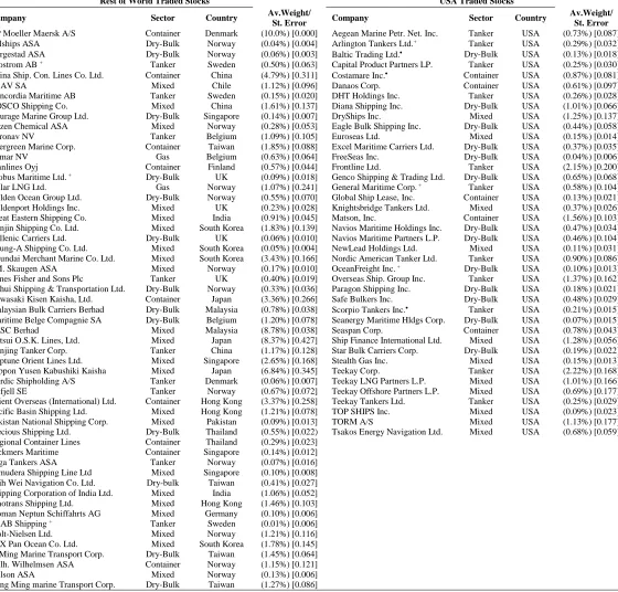
Table 1 describes the composition of the “Shipping” index. The average weights of the

constitu-ents along with their associated standard errors are also reported. To ensure that no company has

an excessive undesirable impact on the index, constituents are confined to a maximum weight of

10%. Any excess weight resulting from the imposed upper bound is distributed proportionately

among the remaining stocks, consistent with their individual market capitalization.

In the empirical analysis, the market-capitalisation-weighted equity index (henceforth

“Shipping” index) and two physical shipping indexes, BDI and BDTI, are to be tracked. DE and

GA are both employed to replicate the performance of the indexes by using a subset of stocks

included either in the Dow Jones Composite Average or the “Shipping” index (henceforth Dow

and Shipping baskets). The stocks picked from the “Shipping” index are used to form the

Ship-ping baskets. Likewise, stocks pulled out from the Dow index form the Dow baskets. For the

pe-riod examined, the average market capitalization of the “Shipping” index components ranges

from $6.7 million to $18.6 billion; the corresponding figure for Dow Jones is $1.4 to $388

bil-lion.

Our investment strategies are devised from the standpoint of a US investor with a

dollar-denominated portfolio. In particular, we examine opportunities in a portfolio composed of either

solely shipping US stocks (Shipping basket) or US stocks in general (Dow basket). This way, we

track the performance of domestic, foreign and physical markets seeking to generate a similar or

improved return-risk profile.

4. EMPIRICAL RESULTS

This section presents the empirical findings on index tracking in the shipping stock and

physical markets. To test the performance of the heuristics, three different scenarios are

exam-ined. In the first one, the algorithms are tested with rebalancing the tracking portfolios for the

out-of-sample period on an annual basis. In the second scenario, the portfolios are rebalanced

12 main purpose of testing these three scenarios is to examine whether the inclusion of additional

information into the index-tracking algorithms—by rebalancing the portfolio more frequently—

is actually more rewarding. In all rebalancing settings, transaction costs are taken into

considera-tion by appropriately adjusting the returns; a 0.75% cost is assumed for each transacconsidera-tion.

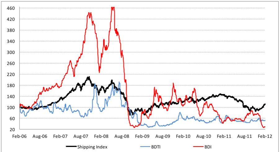
The cumulative returns of the indexes are rebased to 100, and for illustration purposes

they are presented in Figures 1-2. Figure 1 plots the “Shipping” index against three widely

known stock indexes (Dow Jones Composite Average, S&P 500 and NASDAQ 100) and one

commodity index (Dow Jones-UBS). The indexes exhibit similar behaviour, with the “Shipping”

index fluctuating in higher levels, especially before 2009, and also experiencing a more

pro-nounced collapse during the 2008 economic recession. Figure 2 displays the relative

perfor-mances of the “Shipping”, BDI and BDTI indexes. Although the indexes exhibit comparable

trends in the long-run, differences are markedly evident in the short-run. Clearly, the two

physi-cal indexes involve higher levels of volatility with relatively more frequent and large transitory

short-run deviations.

The initial investment budget of our experiments is set equal to C$100, 000. All

track-ing portfolios include at most K stocks, where K can be either 5 or 10. In addition, three

differ-ent trade-off profiles between tracking error and excess return are considered by adjusting the

parameter  in equation (3); the values of  represent different investment attitudes toward

portfolio construction, and are set equal to 0.6, 0.8 and 1. For example, in the case  1, the

in-vestor is interested utterly in pure replication of the index, irrespective of its performance. As 

decreases, the investor is willing to deliberately accept a fraction of the tracking error, in view of

an optimum return-error combination. Implementation of the DE and GA algorithms is repeated

for a series of runs; the ensuing analysis is based on the best reported solution (where the

objec-tive function is minimized) for each particular set of parameters (see Appendix 1, Table A1).

Overall, in terms of tracking errors and excess returns, both DE and GA offer an

analo-gous outcome; yet, results tend to favor the GA, especially when the Dow basket acts as the

tracker. In what follows, we first review the findings on the shipping stock market index

track-ing. Then, the experiment is extended to the shipping physical market. Finally, the tracking

port-folios’ key statistical properties are also discussed, including the reporting of Sharpe ratios,

13

4.1 Tracking the shipping stock market

Figure 3 displays the “Shipping” index against quarterly rebalanced Dow and Shipping

baskets of maximum 10 stocks (K10), with 1 as constructed by the two evolutionary

al-gorithms. These are cumulative returns of the baskets (note that these include reallocation

trans-actions costs of 0.75% per transaction), implying that large errors have an impact throughout the

entire holding period of the out-of-sample period (due to budget constraints, at each point of

re-balancing the index and the tracking baskets differ). Thus, in terms of cumulative return levels

some differences are evident, especially for the shipping baskets. However, both baskets seem to

reasonably track the daily variations of the “Shipping” index. In addition, after the second half of

2008, the Dow basket consistently generates cumulative returns in excess of the benchmark. It

should be stressed out that, although the 2008 financial crisis caused a significant downturn in

the global equity markets, many shipping stocks, as represented by the constructed index and

se-lected baskets, exhibited positive returns until the first half of 2008, reflecting the unanticipated

boom in commodities and freight rates. Nevertheless, shortly after, freight rates also collapsed

and shipping stocks rapidly caught up with the general down-trend. Thus, the Shipping baskets

incurred substantial losses compared to the Dow baskets (see Figure 3).

Table 2 documents the out-of-sample daily root mean squared errors and mean excess

re-turns for the constructed DE and GA baskets. For all K,  combinations and under all

rebalanc-ing scenarios, Shipprebalanc-ing and Dow baskets are marginally different; the average of the Dow basket

RMSEs is 0.1528 compared to 0.01526 for the Shipping basket. In terms of RMSE, the best

tracker is the Shipping GA basket with (K,) = (10, 0.6), when weights are rebalanced on a

monthly basis (Panel C, RMSE = 0.01416). This can be attributed to the high correlation

be-tween the Shipping basket and the benchmark, as the latter basket selects stocks from the

con-stituent list of the “Shipping” index. Moreover, all Shipping baskets are associated with negative

excess returns8, primarily because the shipping industry experienced an unparalleled downtrend

during the examined period. The best model to minimize the objective function of Equation 3 is

the Dow GA basket with monthly rebalancing and (K,) = (5, 0.6); this can be calculated from

the information presented in Table 2 (Eq. 3: f = λRMSE-(1-λ)(ER)

=0.6(0.01482)-(1-0.6)(0.0751/100)=0.0086).

14 Another interesting observation involves the rebalancing frequency of the investment

strat-egies. On average, rebalancing the baskets’ weights leads to improved RMSEs. For instance,

looking at the Shipping GA basket, increasing the rebalancing frequency from annually

(quarter-ly) to monthly causes a 3.4 to 8.6% (2.4 to 5.7%) improvement in the RMSEs. The subsequent

effect from quarterly to monthly is less prominent. Monthly rebalancing produces the best results

in terms of tracking errors, apart from the Dow DE baskets where annual portfolio revisions

seem superior. Still, frequent rebalancing overall trims down excess returns, mainly due to

in-creased transaction costs. Other studies such as Dunis and Ho (2005) noted that a quarterly

port-folio update is preferable to monthly or annual reallocations, where the former has the

shortcom-ing of high transaction costs and the latter is too restrictive. Thus, it is up to the investors’

risk-return appetite to decide whether rebalancing the portfolio monthly—which comes at an extra

cost—is better than less frequent revisions.

For pure replication of the benchmark index, i.e. 1, the lowest tracking error is

achieved by the Shipping GA baskets under all rebalancing strategies. Moreover, different values

of  do not impact RMSEs much. Turning to the mean excess returns, these are maximized for

0.6

 as expected, as the optimization procedure assigns more weight to the target for excess

return. This finding is more pronounced for monthly reallocations; however, any exceptions are

not surprising as the reported metrics for the set of investment strategies are based on the

out-of-sample period. Regarding the efficiency of DE and GA, the latter is associated with lower

track-ing errors and higher excess returns; this is evident when baskets’ readjustments take place more

often, especially in the monthly scheme.

Furthermore, Table 2 presents the results of the SPA tests. We conduct a battery of tests by

grouping the set of tracking portfolios from various aspects. The first objective is to determine

the relative efficiency of the algorithms employed, i.e. whether the tracking errors (RMSEs) are

significantly better for the DE or GA of the same parameters (K and ), baskets (either Dow or

Shipping) and rebalancing periods, using pairwise comparisons. RMSE values with the

super-script “a” attached to them denote the tracking portfolios with significantly better performance

compared to the competing algorithm. Results show that GA significantly outperforms the DE

(24 out of 36 cases), especially for quarterly and monthly rebalanced baskets. The second

objec-tive is to determine the relaobjec-tive efficiency of the replication strategies, i.e. to identify if a model

re-15 balancing scheme; that is, at each row of Table 2. RMSE values with the superscript “b” attached

to them denote the tracking portfolios with significantly better performance compared to the

competing baskets and algorithm, using joint comparison of four models per test. Yet, no

signifi-cantly lower errors can be observed for any particular basket at each set of K,  and

rebalanc-ing period at 5% level (henceforth the considered level of significance examined is 5% for all

SPA tests). This implies that nominal RMSE values are statistically equivalent. In addition, the

above tests are also performed when excess returns (ER) are considered as the objective (and not

the RMSEs). ER values with superscripts “a” or “b” attached represent tracking portfolios with

significantly higher returns compared to the rival algorithm or the rival tracking basket,

respec-tively. Table 2 asserts that the GA is more effective (14 out of 24 cases), whereas only the Dow

GA basket manages to outperform all, the Dow DE, Shipping GA and Shipping DE baskets, at

certain cases (9 out of 18).

Finally, another objective is to verify the relative efficiency of the rebalancing scenarios,

i.e. whether more frequent portfolio revisions lead to significantly lower RMSEs and/or higher

ERs, for each given basket; that is, at each column of Table 2. For that reason, joint comparisons

of 13 strategies are implemented, e.g. annually rebalanced Dow basket with certain K and 

parameters, all monthly and quarterly frequencies of the Dow basket and for all K and .

Re-sults are not presented here and are available from the authors upon request; however, findings

are consistent. Regarding RMSEs, monthly rebalancing generates significantly lower values; this

holds for all GA baskets as well as for the DE baskets with K5. Regarding ERs, overall,

monthly rebalancing produces significantly lower returns, and results are stronger for the DE

baskets.

4.2. Tracking the shipping physical market

The physical shipping index tracking results are reported in Table 3. Clearly, the Dow

bas-kets outperform the Shipping basbas-kets with an average RMSE reduction close to 14%. Moreover,

the Dow baskets accomplish relatively higher excess returns in all cases; an approximate average

increase of 7.6 basis points in ER. Once more, the GA provides a superior combination of excess

returns and RMSEs; on average, excess returns are 1 basis point higher and RMSEs are 2.5

per-centage points lower compared to the DE algorithm. The best out-of-sample BDI tracker is the

16 BDTI it is the Dow basket with (K,) = (10, 0.8) under the same rebalancing frequency (Panel

B, RMSE = 0.02722).

Similar to the shipping stock index tracking exercise, the baskets still generate the highest

excess returns when 0.6, in line with the trade-off criterion (17 out of 24 cases for BDI and 20 out of 24 for BDTI). Once again, it is up to the investors’ preferences to decide on the

trade-off parameter. Moreover, as before, there is a negative relationship between rebalancing

fre-quency, tracking errors and excess returns; frequent revisions increase accuracy at the cost of

higher transaction fees. On the other hand, increasing the rebalancing frequency has a marginal

effect. Finally, should the investor increase the number of stocks included in the basket from

5

K  to K10, the outcome will be only trivially altered. Overall, as highlighted in Table 3

(Panels A and B) the best model to minimize the objective function of Equation 3 is the Dow GA

basket with monthly rebalancing and (K,) = (5, 0.6), as was the case when tracking the

“Ship-ping” index.

The results of the SPA tests are also displayed in Table 3. It can be observed that both BDI

and BDTI can be tracked by the Dow GA baskets with significantly lower tracking errors

(super-script “b”), while GA is generally more accurate (super(super-script “a”). As for excess returns, there

are only few cases where significance is achieved; 24 out of 72 when comparing the algorithms

and 15 out of 72 when comparing the baskets at any given set of parameters K,  and

rebalanc-ing scenarios (however, results are stronger for monthly rebalancrebalanc-ing frequencies: 3 out of 6 for

BDI and all 6 for BDTI). Overall, Dow GA baskets present better ability of replicating the

physi-cal indexes. This evidence is unanimous across RMSEs in all rebalancing scenarios; for excess

returns it is more profound in the monthly rebalancing scheme. Finally, the findings on the

rela-tive efficiency of the rebalancing periods (available from the authors upon request) are similar to

the stock index tracking problem. For BDI, regarding RMSEs (ERs) monthly (annually)

re-balancing produces significantly lower (higher) figures compared to quarterly and annually

(monthly and quarterly). For BDTI, results are mixed between the GA and DE. BDTI GA

bas-kets are associated with significantly lower errors in quarterly and monthly schemes; this does

not hold for DE baskets, where there is no clear winner according to the SPA tests. Still, for ERs,

annually rebalanced baskets are superior.

When comparing the baskets’ performance in terms of tracking the physical and shipping

17 errors, tracking BDI and BDTI is far more challenging. Yet, the less accurate tracking

perfor-mance of the physical market is not startling. It is a consequence of, first, the low correlation

be-tween the physical and financial markets and, second, the existence of diverse and unique to each

market risk factors; these act as further complexities in the effort to mimic the behavior of

physi-cal quantities using financial stocks. Hence, tracking the physiphysi-cal indexes is more demanding

because the physical and stock markets display relative autonomy in their price formation

mech-anisms and evolution. Figures 4 and 5 illustrate the relative performance of the Dow and

Ship-ping baskets in tracking the BDTI and BDI under the genetic and differential evolution

algo-rithms. As in the “Shipping” index case, note that these are cumulative returns of the baskets

(in-cluding reallocation transactions costs of 0.75% per transaction) and large errors have an impact

throughout the complete holding period, i.e. four years (due to budget constraints, at each point

of rebalancing the index and tracking baskets are not the same).

4.3. Statistical properties and risk-return profile of the constructed portfolios

Tables 4 and 5 present key statistics of the constructed baskets, the correlation of the

track-ing portfolio returns with the benchmark returns and the correspondtrack-ing Sharpe ratios. For

com-parison reasons, in Panel D of Table 4, the annualized mean and volatilities of three stock

index-es (Dow Jonindex-es Composite Average, S&P 500 and NASDAQ 100) and one commodity index

(Dow Jones-UBS) are also reported (see also Figure 2). When comparing the Sharpe ratios, only

the commodity index has similar risk-return profile to the shipping markets (negative). The

fi-nancial indexes are able to generate a better risk-return performance compared to the shipping

indexes. According to the historical annualized volatilities, the “Shipping” index exhibits

compa-rable levels of volatility with the other financial indexes; these are in the range of 26.5 to 29%.

Slightly lower is the volatility of the commodity index (23.5%), whereas BDI and BDTI are

as-sociated with fairly elevated levels of volatility. This is due to changing economic and seaborne

transportation patterns, international politics, technological advances, structural changes in the

maritime industry and major events (canal closures, embargoes and wars); all these have created

considerable uncertainty in the shipping physical markets, which strongly depend on demand and

supply fluctuations in seaborne transportation. .

Next, we turn our attention to the different tracking strategies. Moving from annual

18 higher transaction costs. It can be argued that when rebalancing, the additional information

available from the latest price data does make a difference in reducing the portfolios’ volatility,

but the small return deterioration outweighs the volatility benefits. Results are consistent for all

cases for the risk-return trade-off . The best performance for the stock index tracking, in terms

of Sharpe ratios, is reported for the Dow GA baskets that are rebalanced quarterly for (K,) =

(5, 0.6). In that case the reward-to-risk ratio equals 0.414, much higher than the benchmark

“Shipping” index of -0.406. Regarding the physical indexes tracking (see Table 5), the best

per-formance is achieved by the Dow GA baskets that are rebalanced annually for (K,) = (5, 0.6)

for both BDI and BDTI. The corresponding Sharpe ratios of the baskets are 0.357 and 0.535,

whereas the benchmark Sharpe ratios are -1.317 and -0.286, respectively.

Although the Dow baskets generate positive Sharpe ratios, at least in annually and

quarter-ly rebalancing frequencies, this does not hold for “Shipping” baskets. In general, this implies that

the tracked and benchmark indexes present differences in terms of sign (Dow baskets only)

and/or level. On the one hand, for the “Shipping” index differences in the level of annualized

re-turns can be explained by the fact that shipping stock markets have been more vulnerable to the

recent economic recession compared to other equity markets. Hence, shipping-related (Dow)

portfolios over the out-of-sample period underperform (outperform) the benchmark stock index,

as they are associated with lower (higher) annualized returns. On the other hand, physical

mar-kets have been even more susceptible to the recent economic recession, as generally both Dow

and Shipping baskets outperform the benchmark in terms of Sharpe ratios and returns. Interesting

is the case of the Dow baskets which often manage to achieve returns with opposite sign than

that of the tracked indexes. This can be attributed to the relatively lower correlation as well as the

resulting relatively lower volatilities of the Dow baskets, compared to BDI and BDTI. However,

note that more frequent rebalancing, improves tracking performance.

Moreover, for all rebalancing frequencies, Dow baskets volatilities are significantly lower

than the benchmark irrespective of whether this is the “Shipping” index or the BDI, BDTI (an

F-test of equal variances confirms this finding). The Dow baskets experience annualized volatilities

of 17% to 25%, which is less than not only all the benchmark indexes but also the Dow Jones

Composite Index itself. This implies that high diversification benefits may arise, while at the

same time, different combinations can be selected that offer reduced portfolio variance. In the

19 the “Shipping” index with US shipping stocks, no variance reduction is observed. This is not a

surprising result as stocks (K 5 or 10) are selected from a subset (N37) of a much wider

index (N95). Thus, opportunities for potential diversification benefits are rather limited.

Several studies in the literature propose different rules for settingK. Maringer and

Oyewumi (2007) argued that including roughly 50% of the available assets is suitable to get the

desirable properties in the tracking portfolios. Meade and Beasley (2004) suggested that the

op-timum number of stocks in the tracking portfolio should be the minimum number of stocks

need-ed to provide half of the capitalization of the index. However, note that none of the

above-mentioned suggestions apply to our experiment because of the limitation of using US stocks only

from our index (37 US stocks out of 95) or different stocks than the constituents of the

bench-mark index. Moreover, in the case of the physical indexes the traditional approaches do not apply

as we are constrained to use a specific set of stocks to replicate a physical quantity. This can also

explain the relatively low (and in some cases negative) correlations of the selected equity baskets

with the BDI and BDTI (between -4.4% and 14.5%); overall, our results suggest that investors

who want to participate in the physical shipping industry can still benefit from the addition of the

selected baskets to a well-diversified portfolio of assets.

Finally, Table 6 presents the total number of different stocks included in the tracking

bas-kets, throughout the entire out-of-sample period. In any case, by construction, this number

can-not exceed N65 (37) for the Dow (Shipping) baskets9. It can be observed that the GA tends to

utilize more stocks to construct the portfolios. For example the total number of stocks that the

Dow DE (GA) selects to track the “Shipping” index is 19, 30 and 35 (25, 43 and 56) for

annual-ly, quarterly and monthly rebalancing (see Table 6, Panel A: K, = 10, 0.8). For annual

portfo-lio revisions, both algorithms are more stable in the number of stocks picked between the various

cases of the risk/return trade-off, whereas portfolios are quite different in terms of their

composi-tion when increasing the rebalancing frequency.

5. CONCLUSIONS

9 _{For example, consider the annually rebalancing scheme. Starting with the first reallocation period (Feb 2008 to}

Feb 2009), say the algorithm selects K = 4 stocks, namely s1, s2, s3, s4. We count these 4 stocks. In the next period,

Feb 2009 to Feb 2010, say the algorithm selects K = 5 stocks, namely s1, s2, d1, d2, d3. We count only the 3 new

stocks d1, d2 and d3. Thus, for Feb 2008 to Feb 2010 this gives a total of 7 stocks; and so on. In the case of

annual-ly rebalancing (4 rebalancing periods) this number cannot exceed 20 when K = 5 and 40 for K = 10, i.e. at most 5

20 In this paper, we construct an international market-capitalisation-weighted shipping index,

and its performance is reproduced by investing only in a subset of stocks within the index itself

or in a subset of stocks from the Dow Jones Composite Average. We further extend our results to

the case of physical shipping markets. In particular, using the Baltic Dry Index and the Baltic

Dirty Tanker Index as benchmarks, we assess the tracking capability of the same set of stocks. In

our methodology, we employ the differential evolution algorithm and a genetic algorithm. To

test the performance of the heuristics three different rebalancing scenarios are examined: a)

an-nually, b) quarterly and c) monthly. Transaction costs are also taken into consideration.

For the time period under investigation, and irrespective of the rebalancing frequency, the

Dow GA baskets provide the minimum tracking errors and maximum mean excess returns.

Alt-hough the physical shipping markets’ index tracking problem provided similar results, tracking

errors were much higher, mainly due to different return-risk profiles and lower correlations

be-tween the equity and physical maritime segments. Furthermore, better tracking results were

ob-tained with a monthly rebalancing strategy. Looking at Sharpe ratios, it can be noted that

annual-ly (when tracking the BDI and BDTI) and quarterannual-ly (when tracking the shipping index) strategies

perform better; this is attributed to transaction costs trimming down the returns of more frequent

rebalancing strategies. Thus, it is up to the investors’ risk/return preferences to decide whether

rebalancing the portfolio monthly, which comes with an extra cost, is better than less frequent

rebalancing. In addition, volatilities of the constructed portfolios are found to be significantly

smaller for the Dow baskets, especially when tracking the BDI and BDTI. The resulting Sharpe

ratios, with the exception of shipping baskets, are superior not only to the benchmark indexes but

also against other widely traded benchmark financial and commodity indexes. The robustness of

all results is checked by applying predictive ability tests using bootstrap simulations to determine

whether any particular basket outperforms the others in terms of tracking errors and excess

re-turns. The tests focus on the relative efficiency a) of the DE and GA algorithms employed, b) of

the tracking baskets across parameters and rebalancing strategies and c) of the rebalancing

sce-narios.

This paper could encourage mutual and hedge fund managers to set up shipping Exchange

Traded Funds (ETFs) that track our proposed shipping equity index or the two physical indexes.

Similarly, investors, private and institutional, could be motivated to follow a sector of the

21 ETFs could be utilized by ship owners, shipping market participants or other major investors to

complete parts of their investment portfolios or perform tactical investment strategies. To that

end, our proposed methodology puts forward an effective and at the same time least expensive

22

APPENDIX

A.1 Differential Evolution Algorithm

DE is a population-based stochastic optimization algorithm that employs mutation,

recom-bination (crossover) and selection operators to evolve iteratively an initial set (population) of

NP randomly generated N-dimensional solutions. At each iteration (generation), the algorithm

applies the aforementioned evolutionary operators to each one of the available solutions. In

par-ticular, let G i

x denote the solution vector i (i 1, ,NP) at a generationG, x_ijG be the jth

ele-ment of G i

x , and _*G

x the best solution from generation G (specified according to the problem’s

objective function). Having G i

x as the starting basis, a new solution G1

i

x is constructed replacing

G i

x in the next generationG1. The solution updating process is performed in the following

three steps:

1. A mutant solution v_i is constructed by combining xG_i with x_*G and two other randomly

se-lected (different) solutions x and x from the current generation:

*

( ) ( )

 G  G G    

i i F i F

v x x x x x . The mutation constant F(0, 2] controls the rate at

which the population evolves.

2. The parent solution xG_i and the mutant vector v_i are recombined to produce a crossover

so-lution u_i, using the exponential scheme as shown in Figure A1 (for simplicity the generation

index G is not shown in the figure), where l and j* are randomly selected from

{1, 2,, }N , such that the part of u_iderived from v_i is analogous to a user-defined

crosso-ver probability CR (with higher values corresponding to a stronger impact of vi).

3. The crossover solution u_i is compared against the parent vector x_{i G,} on the basis of the

problem’s objective function f . If ( )_i  ( _iG)

f

f u x , then Gi 1



x is set equal to ui (ui replaces

,

i G

x in the next generation); otherwise, G 1

i



x is set equal to G i

x .

The iterative procedure terminates when a stopping criterion is met (e.g., after a predefined

23

... ... ...

Parent solution Mutant solution

Crossover solution

1, 2,,

i i iN

x x x v_i1,v_i2,,v_iN

1

i

x x_i2 x_{i, 1} v_i v_i,1 v_{i j, * 1} x_ij* x_iN

Fig. A1: DE’s exponential crossover scheme.

A.2 Genetic algorithm

Similarly to the DE algorithm, a GA is also a population-based stochastic optimization

pro-cess. It uses the same evolutionary operators, but implements them in a different way and does

not follow the greedy approach adopted by DE. Starting with an initial (random) population of

solutions, the algorithm proceeds iteratively over a number of generations. In the GA

imple-mented in this study, the following algorithmic steps are performed at each iteration (generation):

1. A pair of parent solutions x and y is selected from the current population using a

tourna-ment selection procedure. Under this scheme, k individuals (tournament size) are randomly

selected from the population with replacement, and only the best individual (according to the

problem’s objective function) is selected as a parent.

2. The parent solutions are used to perform the crossover operation with a pre-specified

crosso-ver probability (this probability controls the frequency with which crossocrosso-ver is performed).

Under the arithmetic crossover scheme this operation leads to a new pair of solutions

(1 )

r r

 

 

x x y { , }x y  and y (1 r)xry, where r is a random number drawn from the

uniform distribution in [0, 1].

3. The crossover solutions are subject to mutation. In this study the uniform mutation strategy is

employed, under which p N_m randomly selected elements of a solution vector are replaced

by random values selected uniformly from a pre-specified range. The mutation

probabil-ityp_m controls the frequency of the mutation changes.

The pair of solutions resulting from the mutation operator is placed in the next generation

of solutions, and the above three steps are repeated until the new population is fully formulated.

The procedure ends as soon as a termination criterion is met (e.g., the population converges or

[image:25.612.67.494.113.236.2]

24

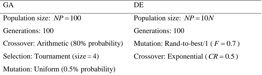
Table A1

Parameters of the algorithms

GA DE

Population size: NP100 Population size: NP10N

Generations: 100 Generations: 100

Crossover: Arithmetic (80% probability) Mutation: Rand-to-best/1 (F 0.7)

Selection: Tournament (size=4) Crossover: Exponential (CR0.5)

25

Acknowledgements

26

REFERENCES

Alexander, C., Dimitriu, A., 2002. The cointegration alpha: Enhanced index tracking and long-short equity market neutral strategies. ISMA Discussion Papers in Finance, 2002-08, ISMA Centre, University of Reading.

Alizadeh, A.H., Nomikos, N.K., 2007. Investment timing and trading strategies in the sale and purchase market for ships. Transportation Research Part B: Methodological 44(1), 126-143. Bao, Y., Lee, T-H., Saltoglu, B., 2006. Evaluating predictive performance of value-at-risk

models in emerging markets: A reality check. Journal of Forecasting 25(2), 101-128. Barber, B.M., Odean, T., 2000. Trading is hazardous to your wealth: the common stock

investment performance of individual investors. The Journal of Finance 55(2), 773-806. Beasley, J.E., Meade, N., Chang, T.-J., 2003. An evolutionary heuristic for the index tracking

problem. European Journal of Operational Research 148(3), 621-643.

Canakgoz, N.A., Beasley, J.E., 2008. Mixed-integer programming approaches for index tracking and enhanced indexation. European Journal of Operational Research 196, 384-399.

Chen, C., Kwon, R.H., 2012. Robust portfolio selection for index tracking. Computers & Opera-tions Research 39, 829-837.

Chang, T-J., Yang, S-C., Chang, K-J., 2009. Portfolio optimization problems in different risk measures using genetic algorithm. Expert Systems with Applications 36(7), 10529-10537. Drobetz, W., Schilling, D., Tegtmeier, L., 2010. Common risk factors in the returns of shipping

stocks. Maritime Policy and Management 37(2), 93-120.

Drobetz, W., Tegtmeier, L., 2011. The development of a performance index for KG funds and a comparison with other shipping-related indices. Working paper, University of Hamburg. Dunis, C.L., Ho, R., 2005. Cointegration portfolios of European equities for index tracking and

market neutral strategies. Journal of Asset Management 6(1), 33-52.

Feoktistov, V., Janaqi, S., 2004. Generalization of the strategies in differential evolution. In: The 18th _{International Parallel and Distributed Processing Symposium, Santa Fe, New Mexico,}

USA.

Frino, A., Gallagher, D.R., 2001. Tracking S&P 500 index funds. The Journal of Portfolio Management 28(1) 44-55.

Gaivoronski, A.A., Krylov, S., Van der Wijst, N., 2004. Optimal portfolio selection and dynamic benchmark tracking. European Journal of Operational Research 163(1), 115-131.

Goldberg, D.E., 1989. Genetic Algorithms in Search, Optimization & Machine Learning. (1st ed.). Addison-Wesley.

Gompers, P.A., Metrick, A., 2001. Institutional investors and equity prices. Quarterly Journal of Economics 116(1), 229-25.

Grammenos, C.Th., Nomikos, N.K., Papapostolou, N.C., 2008. Estimating the probability of default for shipping high yield bond issues. Transportation Research Part E: Logistics and Transportation, 44(6), 1123-1138.

Grammenos, C.Th., Papapostolou, N.C., 2012. Ship finance: US public equity markets. In Talley W. K. (ed.), The Blackwell Companion to Maritime Economics. (1st ed.). Wiley-Blackwell, USA, (chapter 20).

Hansen, P.R., 2005. A test of superior predictive ability. Journal of Business and Economic Sta-tistics 23(4), 365-380.

27 Holland, J. H., 1975. Adaptation in Natural and Artificial Systems. University of Michigan Press.

(1st ed.). Ann Arbor.

Hsu, P.H., Hsu Y-C., Kuan, C.H., 2010. Testing the predictive ability of technical analysis using a new stepwise test without data snooping bias. Journal of Empirical Finance 17(3), 471-484.

Kavussanos, M.G., Alizadeh, M.H., 2002. Seasonality patterns in tanker spot freight rate mar-kets. Economic Modelling 19(5), 747-782.

Kavussanos, M.G, Visvikis I.D., 2006. Derivatives and risk management in shipping. Witherbys Publishing (1st ed.). London.

Killian, L., 2009. Not all oil price shocks are alike: disentangling demand and supply shocks in the crude oil market. American Economic Review 99(3), 1053-1069.

Krink, T., Paterlini, S., 2009. Multiobjective optimization using differential evolution for real-world portfolio optimization. Computational Management Science 8, 157-179.

Krink, T., Mittnik, S., Paterlini, S., 2009. Differential evolution and combinatorial search for constrained index-tracking. Annals of Operations Research 172, 153-176.

Konno, H., Hatagi, T., 2005. Index-plus-alpha tracking under concave transaction cost. Journal of Industrial and Management Optimisation 1(1), 87-98.

Larsen-Jr, G.A., Resnick, B.G., 1998. Empirical insights on indexing. The Journal of Portfolio Management 25(1), 51-60.

Li, Q., Sun, L., Bao, L., 2011. Enhanced index tracking based on multi-objective immune algorithm. Expert Systems with Applications 38, 6101-6106.

Markowitz, H., 1952. Portfolio selection. The Journal of Finance 7(1), 77-91.

Maringer, D., 2008. Constrained index tracking under loss aversion using differential evolution. In: Brabazon, A., O’Neil, M. (eds.), Natural Computing in Computational Finance, Studies in Computational Intelligence 100, Springer, Berlin, 7-24.

Maringer, D., Oyewumi, O., 2007. Index tracking constrained portfolios. Intelligent Systems in Accounting, Finance and Management 15, 57-71.

Malkiel, B., 1995. Returns from investing in equity mutual funds 1971 to 1991. The Journal of Finance 50(2), 549-572.

Meade, N., Beasley, J.E., 2004. An evaluation of passive strategies to beat the index. Working Paper Series, Tanaka Business School.

Merikas, A., Gounopoulos, D., Karli, C., 2010. Market performance of US listed shipping IPOs.

Maritime Economics and Logistics 12(1), 36-64.

Michalewicz, Z., 1994. Evolutionary computation techniques for nonlinear programming problems. International Transactions in Operational Research 1(2), 223-240.

Neuhierl, A., Schlusche, B., 2011. Data snooping and market-timing rule performance. Journal of Financial Econometrics 9(3), 550-587.

Oh, K.J., Kim, T.Y., Min, S., 2005. Using genetic algorithm to support portfolio optimization for index fund management. Expert Systems with Applications 28, 371-379.

Politis, D. N., Romano, J. P., 1994. The stationary bootstrap. Journal of The American Statistical Association 89(428), 1303-1313.

Price, K.V., Storn, R.M., Lampinen, J.A., 2005. Differential Evolution: A Practical Approach to Global Optimization. Springer. (1st ed.). Heidelberg.