1
An artificial neural network based decision support system for energy
efficient ship operations
a*
Bal Beşikçi, E.,
aArslan, O.,
bTuran, O.,
cÖlçer, A.I.
aDepartment of Maritime Transportation Management Engineering, Istanbul Technical University, Sahil Street,
34940,Tuzla, Istanbul, Turkey,
b
Department of Naval Architecture, Ocean and Marine Engineering, University of Strathclyde, 100 Montrose Street, Glasgow G4 0LZ, United Kingdom,
cWorld Maritime University, PO Box 500, SE-20124 Malmö, Sweden.
ABSTRACT
Reducing fuel consumption of ships against volatile fuel prices and greenhouse gas emissions resulted from international shipping are the challenges that the industry faces today. The potential for fuel savings is possible for new builds, as well as for existing ships through increased energy efficiency measures; technical and operational respectively. The limitations of implementing technical measures increase the potential of operational measures for energy efficient ship operations. Ship owners and operators need to rationalise their energy use and produce energy efficient solutions. Reducing the speed of the ship is the most efficient method in terms of fuel economy and environmental impact. The aim of this paper is twofold: (i) predict ship fuel consumption for various operational conditions through an inexact method, Artificial Neural Network ANN; (ii) develop a decision support system (DSS) employing ANN based fuel prediction model to be used on-board ships on a real time basis for energy efficient ship operations. The fuel prediction model uses operating data -‘Noon Data’ - which provides information on a ship’s daily fuel consumption. The parameters considered for fuel prediction are ship speed, revolutions per minute (RPM), mean draft, trim, cargo quantity on board, wind and sea effects, in which output data of ANN is fuel consumption. The performance of the ANN is compared with multiple regression analysis (MR), a widely used surface fitting method, and its superiority is confirmed. The developed DSS is exemplified with two scenarios, and it can be concluded that it has a promising potential to provide strategic approach when ship operators have to make their decisions at an operational level considering both the economic and environmental aspects.
Keywords: Ship Energy Efficiency, Operational Measures, Decision Support System, Artificial Neural Networks
*
Corresponding Author:
Tel: +90 541 7444391
2
1. Introduction
1.1. Ship energy efficiency measures and the importance of developing a decision support system
CO2 emissions generated by maritime transport represent a significant part of total global greenhouse gas (GHG) emissions. According to the International Maritime Organisation (IMO), ships emitted 1016 million tonnes of CO2 on average for the period 2007-2012 which make up approximately 3.1% of global emissions [1].
With the tripling of world trade, if no action is taken, it is assumed that the emissions from shipping will increase by 50% –250% until 2050 [1]. OECD also reported a similar level of prediction in the increase in CO2 emissions from shipping [2].
As there is a strong demand for ships to reduce the emissions, a number of current research activities focus on estimating global shipping emissions and develop mitigating solutions to tackle the problem, e.g. [3–10]. In addition, the rising and volatile fuel prices constitutes a major problem for shipping companies as the fuel cost forms 60% of the ship operating cost [11]. As a result, shipping companies are moving towards energy efficient procedures and operations for reducing energy consumption in order to lower their management costs and thereby maintain their competitive position in the market and to reduce negative environmental impacts.
Ship energy efficiency measures offer various options to ship owners and operators to reduce fuel consumption and emissions. In 2011, IMO’s Marine Environment Protection Committee (MEPC) adopted the amendments to International Convention for the Prevention of Pollution from Ships (MARPOL) Annex VI, as a new chapter (Chapter 4). Through this, Energy Efficiency Design Index (EEDI) for new ships and Ship Energy Efficiency Management Plan (SEEMP) for all ships have been made compulsory from 1 January 2013 [12]. While EEDI facilitates implementation of technical measures through design to meet the carbon emission limits for new ships, SEEMP aims to increase the energy efficiency, through operational applications that are developed using the existing technologies in ships, including crew awareness and training on energy efficiency. For the above reasons, the fuel saving of ships has become paramount for ship energy efficiency.
1.2. Overview and requirements for ship operational energy efficiency decision support system
Decision support systems (DSS) are kinds of computer-based information system that can help decision makers utilize data, models and other knowledge on the computer to solve semi structural and some non-structural problems, which cannot be measured or modelled. This aspect of semi-structured problems requires human intervention, and therefore, solutions to semi-structured problems are often achieved by allowing a decision-maker to select and evaluate practical solutions from a finite set of alternatives. The aim of DSS is to help decision makers improve decision-making effectiveness and efficiency by combining information resources and analysis tools [13].
Combined effects of several factors are involved for evaluating ship operational energy efficiency measures. Determining a strategic implementation becomes more complicated for ship operators due to its complexity and difficulty. There is a need for decision support to provide quickly and directly solution for predicting fuel consumption at an operational level through implementing operational measures using the existing technologies in ships to increase energy efficiency and to decrease environmental effects and overall costs.
3
developing an innovative approach for shipping companies to utilise the noon data for improving the energy efficiency.
1.3. The use of artificial neural networks and related literature
One of the methods used as an alternative to traditional estimation methods is artificial neural network for complex systems [14]. As long as there are adequate samples, the input variables accurately state the output variable through the ‘‘training’’ process of ANN. Considering the nature of data, appropriate methods should be selected to obtain best-fit prediction. This study finds that Artificial Neural Network (ANN) technology is suited for on-site optimization of ship operational measures related energy efficiency.
In quest of emulating the working principles of human brain, ANN is a field of computational science developed over the recent years to deal with the complex systems, which are very difficult or even impossible to model using other analytical and statistical methods. ANN is well suited for prediction purpose as it can approximate successfully any measurable function [15]. The forecasting capabilities of ANN were acknowledged in the past [14]. ANN shows great adaptability, robustness and fault tolerance due to the large number of highly interconnected processing elements [16]. The surface fitting capabilities of ANNs will be essential for our case and this is the reason why ANN was selected to be used for our study [17].
Numerous studies in different disciplines have been undertaken to predict the fuel consumption by using ANN models [18, 19, 20, 21]. ANN has been found to be the domain for many successful applications of prediction tasks, in modelling and prediction of energy-engineering systems [22], prediction of the energy consumption of passive solar buildings [23], developing energy system and forecast of energy consumption [24], and analysis of reduction of emissions [25]. There are also some relevant reports of ANN’s use based on decision support systems in various subjects such as solving the buffer allocation problem in reliable production [26], developing environmental emergency decision support systems [27], risk assessment on prediction of terrorism insurgency [28] and metamodeling of simulation metamodel [29]. ANN has been used to predict specific fuel consumption and exhaust temperature of a Diesel engine for various injection timings [30]. However, no paper is found that modelled fuel consumption using ANN for decision support system based on ship operating data -‘Noon Data’.
1.4. Aim of this study
The study on operations research (OR) in energy modelling and management based maritime transportation had great attention in recent decades. Ronen [31] examined the tradeoff between fuel savings through speed reduction and the loss of incomes as a result of voyage extension. Brown et al. [32] focused a scheduling problem for crude oil tanker and determined optimal speeds for the ships, the best routing of ballast legs and cargo assignment. Perakis and Papadakis [33, 34] decided the fleet deployment and the related optimal speed for ships between one loading port and one unloading port. They later improved their research with multiple loading ports and multiple unloading ports [35]. Yao et al. [36] examined the relationship between bunker fuel consumption rate and ship speed for different sizes of container-ships based on real data obtained from a shipping company.
The majority of these studies focused on speed optimization. To the best of authors’ knowledge, there is no study that takes into account ship’s operating data including speed, trim and weather effects along with decision making in order to minimize ship fuel consumption.
The aim of this paper is twofold: (i) predict ship fuel consumption for various operational conditions through ANN; (ii) develop a decision support system employing ANN based fuel prediction model to be used on-board ships on a real time basis for energy efficient ship operations. The goal of the ANN is to predict ship fuel consumption under various operational conditions using operating data -‘Noon Data’ - which provides information on a ship’s daily fuel consumption.
4
multiple regression analysis (MR), another well-known surface fitting method. Section 6 discusses the design of the (DSS) for improving ship energy. The last section draw conclusions and recommendations for further research.
2. Methods and Data
2.1 Modelling of ship fuel consumption
Ship fuel consumption and its prediction is modelled in three parts: a database of ship fuel consumption obtained from the ship’s noon reports, fuel consumption forecasting algorithm and performance analysis.
To develop ANN based decision support system that can predict ship fuel consumption accurately under various operational factors, a large amount of training and testing data is needed. In the data acquisition, the information and data of ship fuel consumption are acquired mainly from noon reports and also supported by daily reports of the tanker.
Crew fill noon reports every 24 hours at sailing, containing the daily fuel consumption of the ship as well as the daily average of operational details such as draft, speed, duration, distance covered, location, port arrivals, departure, weather, fuel consumption of main engine and auxiliaries along with the type of fuel used. It is compulsory for ship operators to fill these forms. In order to observe and evaluate the changes in the operation systems of ships which sail in various conditions, acquiring daily data is very important. Noon reports are a major indicator of the amount of fuel that ships consume in various weather conditions and at different sailing speeds.
[image:4.595.159.440.470.633.2]The oil tanker used as a case study in this paper spends 51% of her time sailing, 25% at anchor, 11% at port, 9% manoeuvring and 4% drifting. This study is conducted using 233 ship noon reports which have covered the sailing of the ship over the 17 months of her operation since it was built. Table 1 describes the main characteristics of the tanker ship analysed in this study: the ship is equipped with one main engine with internal combustion for propulsion. Metric tonnes per hour (mtons/h) is assumed to be the unit of measurement of fuel consumption in this study as it uses the same basis to compare daily reports in different time intervals.
Table 1
Main characteristics of the analysed ship
Type Oil Tanker
Built 21.6.2012
Length (m) 266.07
Breadth (m) 48
Moulded Depth (m) 23.7
Summer Draft (m) 17
Deadweight (t) 156597
Shaft Power (kw) 18660
Break Horse Power (kw) 25023
Seven important factors - ship speed, revolutions per minute (RPM), mean draft, trim, cargo quantity on board, wind and sea effects- are examined for fuel consumption forecasting model. These are used as inputs in the network training.
5
increasing trade volume per unit time [37]. However, the increase in fuel prices and the environmental problems coupled with global recession have brought a new perspective to ship speed and therefore, lowering the ship speed has become an important research topic.
Reducing the speed of the ship is the most efficient method in terms of fuel economy. According to previous studies, reducing sailing speed by 2-3 knots below the design speed has a considerable impact on daily fuel consumption and thus may halve operating cost of shipping companies [38, 39]. A main reason is that there is a non-linear relationship between ship speed and fuel consumption. The ship speed has a major impact on fuel consumption due to its third-order function with the power consumed by the main engine [31, 40, 41, 42, 43]. This means that, if the ship speed is doubled, the power of the used engine will increase at least eight times. In other words; if the ship speed is reduced by 10%, the amount of fuel consumed by a ship will reduce by about 27% [44].
Speed reduction (slow steaming) has been a major topic in research activities related to low carbon shipping. Notteboom and Vernimmen [45] determined the economic and environmental benefits provided by low speed by examining the relationship between fuel consumption and speed. Corbett et al. [46] have calculated the cost-effectiveness of container ships at low speed. Chang and Chang, [47] applied three different scenarios through speed reductions of bulk carriers by 10%, 20% and 30%. The results indicated that although the low speeds of the ships provide fuel economy, it increases the operating costs because of the low-speed charter contract. Reducing speed is profitable in terms of fuel consumption, it must be balanced in line with other commercial and operational needs, since the reduction of speed means more ships to sustain the same level of service, provided there is a demand.
Liner service ships (container and ferries) are strongly dependent on schedule and port rotation and sail at a given speed [48, 49, 50, 51, 52, 53, 54, 55, 56, 57]. The high penalties resulting from being late have restrained the low speed voyage of these type of ships and therefore fuel economy. For the tramp service ships (tankers and bulk carriers), the ship speed shall be determined in accordance with the estimated time of arrival (ETA). In these types of contracts, the flexibility can occur as a result of delays that may arise due to the port rules or port congestion. If the ship sails at a lower speed instead of waiting for a long time to enter the port (due to congestion at the port), it can reduce the fuel consumption by up to 10% during the voyage [58, 59]. In order to benefit from such situations, dynamic voyage planning is an essential for low carbon shipping.
Revolutions per minute (RPM) is a main engine speed. The engine will run efficiently at the rated RPM at the rated load. When the engine itself is operating at its most efficient, particularly at engine speeds approaching the maximum number of revolutions per minute (RPM), this affects to give a relatively poor fuel consumption rate.
The fuel consumption is also affected by ships' trim and draft. Hull forms traditionally have been designed in accordance with the specific drafts. If the trim of the ship is even slightly different than the design point, the ship resistance might increase and thus fuel consumption. In some circumstances, lighter drafts at the wrong trim may cause higher resistance than a deeper draft at the proper trim [60]. The optimum trim can be provided through the proper distribution of cargo, ballast and consumables by ship's captains and cargo planners. On the other hand, increasing the quantity of cargo increases the draft and displacement of the ship resulting in greater resistance and hence higher fuel consumption.
Ship weather routing is defined as determining the optimum route by taking into account the weather conditions (wind, current and sea effects) on the designated voyage [61, 62, 63]. The optimum route designated for the voyage is considered as the route that allows the completion of the voyage as soon as possible in which the safety and comfort [64, 65], maximum energy efficiency in various weather conditions [66, 67, 68], or a combination of these factors [69, 70]. Published studies, based on real operational data, indicate that it is possible to reduce the fuel consumption by up to 3% by adopting weather routing plans [71].
6
2.2 Artificial Neural Network (ANN)
ANN is one of the most powerful computational methods broadly inspired from the biological nervous systems of the human brain, can achieve remarkable results where the other traditional statistical methods could not be effective.
The ability of learning by example is probably the most important property associated with neural networks and can be used to train a network with the records of past response of a complex system [72].
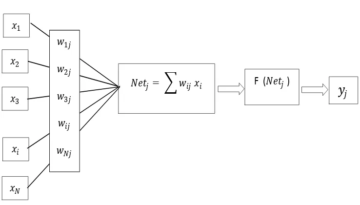
Artificial neural networks are made up many highly inter-connected processing elements called neurons. The basic elements of a neuron is depicted in Figure 1. Artificial neuron mainly consists of weight, bias and activation function. Each neuron receives inputs x1, x2,..., xn, attached with a weight xi which indicates the
connection strength for a particular input for each connection. Then it multiplies every input by the corresponding weight of the neuron connection. A bias bi can be defined as a type of connection weight with
a constant nonzero value added to the summation of inputs and corresponding weights u, given as follows:
𝑢𝑖 = ∑𝑛 𝑊𝑖𝑗
𝑗=1 𝑋𝑗+ 𝑏𝑖 (1)
where ui is the net inside activity level of ith neuron, wij is the jthweight value of the ith layer, xj is the
output value of the jth layer, and n is the number of the neurons.
The activation function yi will create an actual output. It uses a hyperbolic tangent sigmoid transfer
function. The summation ui is transferred using a scalar-to-scalar function called an ‘‘activation or transfer function”, f(ui), to yield a value called the unit’s ‘‘activation”, given as:
[image:6.595.100.469.379.589.2]𝑦𝑖 = 𝑓(𝑢𝑖) (2)
Figure 1: Basic elements of an artificial neuron
The most commonly used training algorithm for the multi-layer perception is a back propagation algorithm (BPA) [73]. It is a gradient descent method to minimize the error for a particular training pattern. The back-propagation stage is carried out through a large number of training sets or training cycles (epochs). These learning processes are repeated until the optimal set of weights, which in the ideal case would produce the right output for any input.
3. Design of ANN Model
In this study, a neural network model has been implemented with Neural Network toolbox presented in MATLAB 2010a.
𝑦
𝑗𝑥1
𝑥2
𝑥3
𝑥𝑖
𝑥𝑁
𝑁𝑒𝑡𝑗 = 𝑤𝑖𝑗 𝑥𝑖 F (𝑁𝑒𝑡𝑗 )
𝑤1𝑗
𝑤2𝑗
𝑤3𝑗
𝑤𝑖𝑗
7
[image:7.595.35.450.188.357.2]The data set derived from 233 noon reports are used to design and construct the ANN. Initially, a sample of 164 (70%) of noon reports was randomly selected for training, and the remaining sample of 69 (30%) of the data was used for validation. There are seven input variables; ship speed, revolutions per minute (RPM), mean draft, trim, cargo quantity on board, wind and sea effects. The output parameter of the ANN model is ship fuel consumption (mtons/h). The range of the samples is given in Table 2.
Table 2
Range of input–output parameters in training–testing phase
Parameters Range of values
Min Max
Ship Speed (knots) 8.69 16.46
RPM 49.16 85
Mean Draft (meter) 7.5 17
Trim (meter) 0 3.2
Carqo Quantity (mton) 0 149419
Wind Effects* (knots) -41.54 36.9
Sea Effects * (meter) -9.14 8.79
Fuel Consumption (mtons/hour) 0.58 3.13
*Vectors: (- indicates adversely effect on fuel savings)
The modelling method for ANN is based on the back-propagation learning algorithm used in feed forward with one hidden layer. A primary task of ANN studies is to identify the ideal network architecture, which is related to the number of hidden layers and neurons in it. Considering the ANN performance, the number of hidden layer(s), the neurons in the hidden layer(s) and the value of the training parameters for every training algorithm were determined through a trial and error method. The optimal architecture of the ANN was constructed as, 7–12–1 NN architecture for fuel prediction representing the number of inputs, neurons in hidden layers, and outputs, respectively. The proposed ANN model is given in Figure 2. The learning algorithm used in the study is Levenberg–Marquardt (LM), activation function is hyperbolic tangent sigmoid transfer functions (inputs and outputs were scaled between -1 and +1 for the neural network model) and number of epochs is set to 10,000.
Figure 2: The schematic of ANN structure
n1
n2 n3 n4
n12
Fuel Consumption (mtons/h) Ship Speed
RPM
Mean draft
Trim
Cargo Quantity
Sea Effects Wind Effects
B1
B2
[image:7.595.143.465.522.755.2]8
Determination coefficient (R2) and error variance criteria (MSE and RMSE) have been used for measuring ANN's performance. The most widely used error indicator, the MSE, of the prediction over all the training patterns for a one output neuron network can be formulized as:
MSE = 2𝑁1 ∑ ( 𝑡𝑁𝑖 𝑖− 𝑧𝑖)2 (3)
N is the total number of training patterns where ti and zi are the predicted output for the ith training pattern
and the target [74]. Another error estimation criterion is the RMSE (root mean square error) and through it, the error is shown in the units of target and predicted data. According to these criteria, high R2 and low MSE and RMSE values are indicating a well-fitting model.
4. Performance of the ANN Model
[image:8.595.142.469.449.707.2]In this section, the results and system efficiency used in forecasting the fuel consumption of a ship will be described. As shown in Table 3, the field study revealed that 1.89 mtons/h of fuel, on average, was consumed by the ship.
Table 3
Statistics of fuel consumption (mtons/h)
Min. Max. Mean SD 95% confidence
interval
Lower Upper
mtons/h 0.58 3.13 1.89 0.50 1.80 1.98
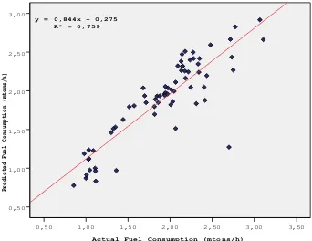
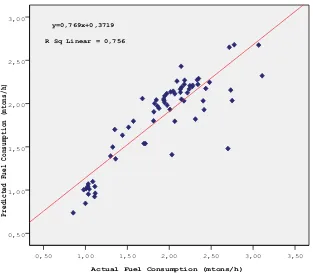
Figure 3 and 4 illustrate the training and validation of the ANN model for observed and predicted values for fuel consumption. The R2 was 0.834 and 0.759 for training and validation of the ANN model, respectively.
Figure 3: Relationships between actual and predicted fuel consumption (Training) using the ANN model
Actual Fuel Consumption (mtons/h)
3,50 3,00
2,50 2,00
1,50 1,00
0,50
Predicted Fuel Consumption (mtons/h)
3,00
2,50
2,00
1,50
1,00
0,50
9
Figure 4: Relationships between actual and predicted fuel consumption (Validation) using the ANN model
ANN technique is treated as black-box application in general. However, this study opens this black box and introduces the ANN application in a closed form solution. This study aims to present the closed form solution of fuel consumption based on the trained ANN parameters (weights and biases) as a function ship speed, revolutions per minute (RPM), mean draft, trim, cargo quantity on board, wind and sea effects.
where the hyperbolic tangent (tan h) transfer function used for this approach is given as follows:
tan ℎ(𝑈𝑖) =1+𝑒−𝑢𝑖
1−𝑒−𝑢𝑖 (4)
where U are given in Eq. (5). The normalization values of input parameters used for Eq. (5).
𝑈𝑖= 𝐶1𝑖× 𝑠ℎ𝑖𝑝 𝑠𝑝𝑒𝑒𝑑 + 𝐶2𝑖× 𝑅𝑃𝑀 + 𝐶3𝑖× 𝑑𝑟𝑎𝑓𝑡 + 𝐶4𝑖× 𝑡𝑟𝑖𝑚 + 𝐶5𝑖× 𝑐𝑎𝑟𝑔𝑜 𝑞𝑢𝑎𝑛𝑡𝑖𝑡𝑦 + 𝐶6𝑖× 𝑤𝑖𝑛𝑑 𝑒𝑓𝑓𝑒𝑐𝑡 + 𝐶7𝑖× 𝑠𝑒𝑎 𝑒𝑓𝑓𝑒𝑐𝑡 + 𝑏𝑖 (5)
where, K are given in Eq. (6) used for Eq. (7)
𝐾𝑖 = ∑𝑛=12İ=1 tan ℎ(𝑈𝑖)×lw𝑖+ 𝑏2 (6)
where, the weights and biases between input layer and hidden layer are given in Table 4 for LM algorithm with 12 neurons.
Actual Fuel Consumption (mtons/h)
3,50 3,00
2,50 2,00
1,50 1,00
0,50
Predicted Fuel Consumption (mtons/h)
3,00
2,50
2,00
1,50
1,00
0,50
[image:9.595.138.480.40.304.2]10
Table 4
The weights and biases between input layer and hidden layer for Eqs. (5) and (6).
n C1i C2i C3i C4i C5i C6i C7i lw b1 b2
1 -0.7431 -0.0587 -0.5878 0.80046 -0.7439 1.2996 -0.417 -0.3347 2.0881 -0.2226
2 -0.5483 1.1236 0.43986 0.65012 0.71865 1.6052 0.03826 0.48388 -1.4265
3 -0.5352 0.32488 0.75197 -0.9981 0.84385 -0.9504 0.19942 -0.8794 -0.9295
4 -0.0148 1.2529 -0.2573 0.99103 -0.6864 0.62122 -0.9913 -0.1947 1.0954
5 1.1545 1.3696 0.71883 0.59309 -0.5946 0.34136 0.84336 -0.4167 0.83542
6 0.00326 0.00296 1.3981 -0.0773 -1.4224 0.08862 -0.1686 0.3915 0.0096
7 0.26818 1.336 0.72698 -0.9393 0.57327 -0.0808 -0.3688 0.61318 -0.1373
8 -0.6215 -1.1863 -0.529 -0.4208 -0.6297 1.5299 -1.3653 -0.3507 -0.5414
9 -0.3622 1.1819 -1.0303 0.50076 0.35171 -1.716 -1.2242 0.54683 1.2775
10 0.29539 0.33189 -0.9563 -1.8743 -0.4322 -0.2218 0.36101 0.70683 1.4561
11 0.50702 -0.3649 0.76347 1.5718 0.63403 0.34273 0.77075 0.56254 1.5673
12 -0.6832 -0.5465 0.33544 1.0733 -0.3552 1.0141 -0.7989 0.46534 -2.1906
Using weights and biases of trained ANN model, the normalized value of fuel consumption can be given as follows:
𝑦𝑖 = 𝑓(𝑢𝑖) =1+𝑒1−𝑒−𝐾𝑖−𝐾𝑖 (7)
where, 𝑦𝑖 is a normalization value and should be converted to actual value of fuel consumption.
Figure 5: Relationships between actual and predicted fuel consumption (Training) using MR model
Actual Fuel Consumption (mtons/h)
3,50 3,00
2,50 2,00
1,50 1,00
0,50
Predicted Fuel Consumption (mtons/h)
3,00
2,50
2,00
1,50
1,00
0,50
[image:10.595.143.467.436.708.2]11
5. Validation and Benchmarking
In this section, the results using the ANN developed above are compared with multiple regression analysis (MR).
One of the most common techniques which are used to determine the relationship between variables in the studies is the regression analysis technique. Multiple regression analysis (MR) is a linear statistical technique which is used for establishing the best relationship between a variable (dependent, predicant) and several other variables (independent, predictor) using the least square method. A multiple regression analysis model is then developed for predicting the fuel consumption as:
Y = a0+ a1V1 + a2V2 + ⋯ + anVn+ ε (8)
where a0-an are the regression coefficients, V1-Vn are the independent variables, and ε is model error. The
model has a linear form in order to represent linear relationships between the dependent variable and the independent variables as well as relationships between independent variables.
It is important to consider the goodness-of-fit and the statistical significance of the estimated parameters of the developed regression models. A model with the highest R2 can be designed through a combination of forward, backward and stepwise regression adjustments. The variables significant at P= 0.05 are always maintained for the final model [75].
MR has been performed under IBM SPSS Statistics 21.0 software. Multiple regression with the highest R2 can be designed in this study through enter method.
The performance was assessed using the same data sets excluding the variable of cargo quantity due the high correlation with the variable draft which causes multicollinearity problem, as were used for examining the performance of the ANN.
[image:11.595.85.512.525.618.2]The linear relationships of the dependent variable with the independent variables are represented by a multiple regression analysis model. Same data sets was used for the training of the ANN in order to compare more comprehensively with the ANN model and predictions on validation data were estimated after running the model. A multiple regression analysis model could be fitted to fuel consumption data and accounted for around 75% of the variance in validation data. Figures 5 and 6 compare the predicted and actual ship's fuel consumption for training and validation data, respectively. The final MSE and RMSE for validation data were 0,038 and 0,196 mtons/h respectively given in table 5.
Table 5
MSE and RMSE for training and validation of the MR and ANN models.
MR ANN
Training Validation Training Validation
MSE 0.03 0.038 0.02 0.037
12
Figure 6: Relationships between actual and predicted fuel consumption (Validation) using MR model
For both training and validation data, the correlation between the actual and predicted energy consumption for the ANN model was shown to be much higher than the correlation for the linear regression model by the comparison done between ANN model and multiple linear regression models; furthermore, RMSE of the ANN model on the validation data was much lower than that of the MR model. (Table 5)
6. Design of the Decision Support System (DSS) for improving ship energy efficiency
Ship operators, making decisions concerning the implementation of operational measures to improve ship energy efficiency, could use with advantage the results obtained from the developed ANN of Section 4.
[image:12.595.76.514.539.718.2]Table 6 shows the seven parameters and their controllability by ship operators for decision support.
Table 6
The parameters can be controlled by ship operators
Inputs Controlled? Description
Ship Speed Ship speed can be increased or decreased considering voyage plan
RPM RPM can be increased or decreased considering voyage plan Cargo
Quantity - Cargo Quantitity is determined by trading parties. Draft - Draft is entered depending on the ship's displacement Trim Trim can be adjusted according to draft.
Wind Effects Wind effect can be decreased with weather routing (course alteration)
Sea Effects Wind effect can be decreased with weather routing (course alteration)
Accordingly;
Actual Fuel Consumption (mtons/h)
3,50 3,00
2,50 2,00
1,50 1,00
0,50
Predicted Fuel Consumption (mtons/h)
3,00
2,50
2,00
1,50
1,00
0,50
13
Ship operator can adjust speed and RPM with consideration of voyage plan (time constraint may occur due to the trading environment). Cargo quantity determines the displacement of ship, so cargo quantity and draft parameters are uncontrollable, only used for prediction. Trim can be optimized according to draft. Wind and sea effects can be used in support of fuel savings by weather routing.
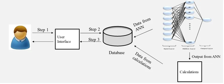
[image:13.595.87.533.132.299.2]The design of this DSS (from the effects of ship operational energy efficiency measures on fuel consumption forecasted by the use of ANN) is shown in Figure 7.
Figure 7: Design of ship operational energy efficiency ANN DSS
The database of DSS contains data from the developed ANN. This ANN was run having as input the seven important impact factors(ship speed, revolutions per minute (RPM), mean draft, trim, cargo quantity on board, wind and sea effects) and the result of the ANN for all these 2337 different input samples were recorded and stored in the database of DSS. It should be noted that; instead of having the results of the ANN for the 2337 different cases stored in the database, the ANN itself could be inserted in the DSS. In this way, based on the user’s input, the ANN would produce dynamically its output on a real time basis.
The ANN based DSS functionality follows these steps:
Step 1: The ship operator enters all the necessary variables including input parameters for ANN and other essential parameters for the voyage of ship such as distance between ports, required date for cargo delivery and the course of ship following prompts from the system.
Step 2: Depending on the input of the ship operator, the system makes the necessary queries to the database.
Step 3: The results of the queries are returned and are presented to the ship operator, who can evaluate them. The user, at this point, can either finish the interaction or continue by returning to Step 1.
To illustrate the functionality of the developed DSS, hypothetical case with two scenarios are presented below, corresponding to ship speed and RPM optimization decision-making situations due to their great significant impacts on fuel savings.
The ship operator enters parameters for draft, trim, cargo quantity, wind and sea effects used for ANN and additional information such as the distance between ports in nautical mile (d) and required date for cargo delivery. In order to evaluate two scenarios for speed and RPM optimization, ship operator enters two different speed and RPM values to receive the outputs of ANN based DSS. (Step 1)
The ship is ballasted condition with 7.5 m draft and 2.7 m trim. Weather adversely affects for wind is 23 knots and sea is 0.3 m. The distance between ports is 800 nautical mile. Ship speed is 10 knots and RPM is 55 for Scenario 1 while ship speed is 13 knots and RPM is 71 for Scenario 2.
ANN calculation is performed when operational information is input to the interface. Then, the outputs (fuel consumptions) are 0.96 mtons/hour for Scenario 1 and 2.1 mtons/hour for Scenario 2. (Step 2)
Table 7 gives the results of decision support information. The emission factor of CO2 is 3.17 [76, 77, 47]. The fuel price is $150 per metric ton used for calculating the total amount of fuel cost for voyage [46].
User Interface
n1 n2 n3 n4
n12
Input Layer Hidden Layer Output Layer
Step 1 Step 2
Step 3
Database
Calculations
14
Table 7
Decision support information
Scenario d (NM) t (hours) Output FC
(mtons/h) Q (mtons) P ($)
CO2 (tons)
Scenario 1 800 80 0.96 76.8 15360 243.456
Scenario 2 800 61.5 2.1 129.15 25830 409.406
where, t is the sailing duration based upon cargo delivery date, Q and P are the total amount of fuel consumption in metric tonnes and fuel cost in dollars for the voyage, respectively.
According to the obtained information, decision maker can manage the operational parameters for decision support. The input information will change according to operational information and requirements considering voyage plan of ship and decision support information will change according to changes in the input information. Ship operator is concerned with the optimum speed and RPM that a ship can reach the port on time. (Extra waiting durations for cargo at anchorage or port as a result of high speed ships or delay for cargo due to the slow steaming are not intended) Thus, ship speed and RPM can be optimized through adjusting sailing duration (t) considering required date for cargo delivery. In this hypothetical case, the difference between two scenarios are approximately 52 metric tons of fuel consumption, 10470 dollars of fuel cost and 165 tons of CO2 for present voyage with 800 nautical mile (NM) distance. The user, after receiving the information shown in table 7, can either continue with an additional investigation concerning a new operational values for different speed and RPM or exit from the system. (Step 3)
7. Conclusion
In terms of ship energy efficiency, fuel consumption has become a primary concern. The lowering of fuel consumption is considered to be the paramount goal as a result of economic pressure and environmental regulations. The potential for fuel savings is possible for existing ships through operational measures.
The overall purpose of this paper is to develop an Artificial Neural Network (ANN) based decision support system for ship operators in making decisions concerning the implementation of operational measures considering both the economic and environmental aspects to improve ship energy efficiency.
This research has demonstrated two novelties; the first one is predicting ship fuel consumption by employing an inexact approach, ANN. The second one is to develop a decision support tool to help ship personnel making optimal decisions on a real time basis for energy efficient ship operations.
This study is the first time an ANN model is designed to predict fuel consumption in ship operations using ships noon report data. With this motivation, the proposed method can be considered as a successful decision support tool for ship operators in forecasting fuel consumption based on different daily operational conditions.
The proposed decision support system provides a strategic approach when ship operators have to make their decisions at an operational level considering both the economic and environmental aspects.
The obtained results make it clear that the neural network can learn very accurately the relationships between the input variables and a ship's fuel consumption. Furthermore, ANN provides relatively better prediction results for ship fuel consumption when compared to the results derived using the MR model.
The developed DSS including the prediction model can also be used during ship design to assess fuel consumption and environmental aspects for design alternatives.
15
a high number of uncontrollable parameters, not only MR model but also other prediction models will be required for improving the accuracy. In addition, the other decision support systems can be developed for different types of ships such as bulk carriers, containers and etc. and larger number of ships with various characteristics.
Acknowledgement
Elif BAL acknowledges Scientific and Technical Research Council of Turkey (TUBİTAK) for a 2214/A-International Research Fellowship Programme and BAP-ITU (Scientific and Projects-ITU). Elif BAL, Ozcan ARSLAN and I. Aykut OLCER acknowledges support from the International Association of Maritime Universities, under project IAMU FY 2014.
References
[1] Third IMO GHG Study. London: International Maritime Organization (IMO); 2014.
[2] OECD Globalization, Transport and the Environment. 2010, ISBN 978-92-64-07290-9.
[3] Walsh, C., Bows, A. Size matters: Exploring the importance of vessel characteristics to inform estimates of shipping emissions, Applied Energy 2012; 98: 128–137.
[4] Gilbert, P., Bows,A., Exploring the scope for complementary sub-global policy to mitigate CO2 from shipping, Energy Policy 2012; 50: 613–622.
[5] Lindstad, H., Asbjørnslett, B.E., Strømman, A.H., The importance of economies of scale for reductions in greenhouse gas emissions from shipping, Energy Policy 2012; 50: 613–622.
[6] Eyring V, Isaksen IS, Berntsen T, Collins WJ, Corbett JJ, Endresen O, et al. Transport impacts on atmosphere and climate: shipping. Atmos Environ 2009;44(37):4735–71.
[7] Entec. Quantification of emissions from ships associated with ship movements between ports in the European Community. UK: Report prepared for the European Commission; 2002. <http://ec.europa.eu/environment/air/pdf/ chapter2_ship_emissions.pdf> accessed 05.01.14.
[8] Entec. Service contract on ship emissions: 2 assignment, abatement and market-based instruments task 2b and c – NOx and SO2 abatement. UK: Report prepared for the European Commission; 2005. <ec.europa.eu/environment/air/ pdf/task2_so2.pdf> accessed 14.01.14.
[9] Endresen Ø, Sørgård E, Sundet JK, Dalsøren SB, Isaksen ISA, Berglen TF, et al. Emission from international sea transportation and environmental impact. J Geophys Res 2003;108:4560.
[10] CE Delft. Technical support for European action to reducing greenhouse gas emissions from international maritime transport. The Netherlands: Report to European Commission; 2009. <http://ec.europa.eu/clima/policies/transport/ shipping/studies_en.htm> accessed 10.12.13.
[11] Golias, M.M., Saharidis, G.K., Boile, M., Theofanis, S., Ierapetritou, M.G., 2009. The berth allocation problem: optimizing vessel arrival time. Maritime Economics & Logistics 11, 358–377.
[12] IMO, Resolution MEPC.203(62), MEPC 62/24/Add.1 Annex 19, 2011. Amendments to the Annex Of The Protocol Of 1997 To Amend The International Convention for the Prevention Of Pollution From Ships, 1973, As Modified by the Protocol Of 1978 Relating Thereto.
[13] Chen, W. Tutorial of Decision Support Systems. Tsinghua University Press, Beijing, China (in Chinese); 2004.
[14] Zhang, G, Patuwo, G. E, Hu, M. Y.Forecasting with Artificial Neural Networks: The State of The Arts. International Journal of Forecasting 1998; 4(1):35.
[15] Hornik K, Stinchocombe M, White H. Multilayer feedforward networks are universal approximators. UK: Elsevier Science Ltd Oxford 1989; 2(5).
16
[17] He, X., Li, C., Hu, Y., Zhang, R., Yang, S. X., & Mittal, G. S. Automatic sequence of 3D point data for surface fitting using neural networks. Computers and Industrial Engineering 2009; 57(1), 408–418.
[18] Togun, NK and Baysec, S. Prediction of torque and specific fuel consumption of a gasoline engine by using artificial neural Networks. Applied Energy 2010; 87:349–355.
[19] Ajdadi, FR, Gilandeh, YA.Artificial Neural Network and stepwise multiple range regression methods for prediction of tractor fuel consumption. Measurement 2011; 44:2104–2111.
[20] Wu, JD, Liu, JC. Development of a predictive system for car fuel consumption using an artificial neural network. Expert Systems with Applications 2011; 38: 4967–4971.
[21] Safa, M, Samarasinghe, S. Modelling fuel consumption in wheat production using artificial neural Networks. Energy 2013; 49:337-343.
[22] Kalogirou SA. Applications of artificial neural-networks for energy systems. Applied Energy 2000; 67:17–35.
[23] Kalogirou SA, Bojic M. Artificial neural-networks for the prediction of the energy consumption of a passive solar-building. Energy 2000;25: 479–91.
[24] Amirnekooei, K., Ardehali, M.M., Sadri, A., Integrated resource planning for Iran: Development of reference energy system, forecast, and long-term energy-environment plan. Energy 2012; 46:374-385.
[25] Ozer, B., Görgün, E., İncecik, S., The scenario analysis on CO2 emission mitigation potential in the Turkish electricity sector: 2006–2030. Energy 2013; 49:395-403.
[26] Tsadiras, A.K., Papadopoulos, C.T, Kelly , M.E.J. O., 2013. An artificial neural network based decision support system for solving the buffer allocation problem in reliable production lines. Computers & Industrial Engineering 66, 1150–1162.
[27] Liao, Z., Wang, B., Xiaa, X., Hannam, P.M., 2012. Environmental emergency decision support system based on Artificial Neural Network. Safety Science 50, 150–163.
[28] Kengpol,A., Neungrit, P., 2014. A decision support methodology with risk assessment on prediction of terrorism insurgency distribution range radius and elapsing time: An empirical case study in Thailand. Computers & Industrial Engineering 75, 55–67.
[29] Can, B., Heavey, C., 2012. A comparison of genetic programming and artificial neural networks in metamodeling of discrete-event simulation models. Computers & Operations Research 39, 424–436.
[30] Parlak, A., Islamoglu, Y., Yasar, H. and Egrisogut, 2006. A., Application of artificial neural network to predict specific fuel consumption and exhaust temperature for a Diesel engine. Applied Thermal Engineering 2006; 26: 824–828.
[31] Ronen, D. The effect of oil price on the optimal speed of ships.Journal of the Operational Research Society 1982; 33:1035–1040.
[32] Brown GG, Graves GW, Ronen D. Scheduling ocean transportation of crude oil. Management Science 1987;33(3):335–4.
[33] Perakis AN, Papadakis NA. Fleet deployment optimization models. Part 1. Maritime Policy and Management 1987;14(2):127–44.
[34] Perakis AN, Papadakis NA. Fleet deployment optimization models. Part 2. Maritime Policy and Management 1987;14(2):145–55.
[35] Papadakis NA, Perakis AN. A nonlinear approach to the multiorigin, multi-destination fleet deployment problem. Naval Research Logistics 1989;36:515–28.
[36] Yao, Z., Ng, S.H., Lee, L.H. A study on bunker fuel management for the shipping liner services. Computers & Operations Research 2012; 39: 1160–1172.
17
[38] Wijnolst, N., Wergeland, T., 1997. Shipping. Delft University Press, Delft.
[39] Stopford, M., 1999. Maritime Economics, Second Edition Routeledge, London.
[40] Fagerholt, K, Laporte, G, Norstad, I. Reducing fuel emissions by optimizing speed on shipping routes. Journal of the Operational Research Society 2010; 61:523–529.
[41] Norstad, I, Fagerholt, K, Laporte, G.Tramp ship routing and scheduling with speed optimization. Transportation Research Part C 2011; 19:853–865.
[42] Cariou, P. Notes and comments. Is slow steaming a sustainable means of reducing CO2 emissions from container shipping? Transportation Research Part D 2011;16: 260–264.
[43] Qi, X, Song, DP.Minimizing fuel emissions by optimizing ship schedules in liner shipping with uncertain port times.Transportation Research Part E 2012; 48: 863–880.
[44] Faber, J, Nelissen, D, Hon, G. Wang, H. and Tsimplis, M.; Regulated Slow Steaming in Maritime Transport: An Assessment of Options. Costs and Benefits 2012; 7:442-1.
[45] Notteboom, T, Vernimmen, B. The effect of high fuel costs on liner service configuration in container shipping. Journal of Transport Geography 2009;17(5):325-337.
[46] Corbett, J, Wang, H, Winebrake, J. The effectiveness and costs of speed reductions on emissions from international shipping. Transportation Research Part D 2009; 14:539-598.
[47] Chang, C.C., Chang,C.H., Energy conservation for international dry bulk carriers via vessel speed reduction. Energy Policy 2013; 59: 710–715.
[48] Christiansen, M., Fagerholt, K., Ronen, D., Ship routing and scheduling: status and perspectives. Transportation Science 2004; 38 (1): 1–18.
[49] Shintani, K., Imai, A., Nishimura, E., Papadimitriou, S., The container shipping network design problem with empty container repositioning. Transportation Research Part E 2007; 43 (1): 39–59.
[50] Gelareh, S., Nickel, S., Pisinger, D., Liner shipping hub network design in a competitive environment. Transportation Research Part E 2010; 46 (6): 991–1004.
[51] Gelareh, S., Pisinger, D., Fleet deployment, network design and hub location of liner shipping companies. Transportation Research Part E 2011; 47 (6): 947–964.
[52] Meng, Q., Wang, S., Liner shipping service network design with empty container repositioning. Transportation Research Part E 2011; 47: 695–708.
[53] Meng, Q., Wang, S., Optimal operating strategy for a long-haul liner service route. European Journal of Operational Research 2011; 215: 105–114.
[54] Wang, S., Wang, T., Meng, Q., A note on liner ship fleet deployment. Flexible Services and Manufacturing Journal 2011; 23 (4): 422–430.
[55] Wang, S., Meng, Q., Schedule design and container routing in liner shipping. Transportation Research Record 2011; 2222: 25–33.
[56] Wang, S., Meng, Q., Liner ship fleet deployment with container transshipment operations. Transportation Research Part E 2012; 48 (2): 470–484.
[57] Wang, S., Meng, Q., Sailing speed optimization for container ships in a liner shipping network. Transportation Research Part E 2012; 48: 701–714.
[58] IMO, MEPC 61/INF.18, 23 July 2010. Reduction Of Ghg Emissions From Ships. Marginal Abatement Costs And Cost-Effectiveness Of Energy-Efficiency Measures.
[59] Norlund, E.K., and Gribkovskaia , I., Reducing emissions through speed optimization in supply vessel operations, Transportation Research Part D 2013; 23: 105–113.
18
[61] Padhy CP, Sen D, Bhaskaran PK. Application of wave model for weather routing of ships in the North Indian Ocean. Natural Hazards 2008; 44:373–85.
[62] Shao W, Zhou PL, Thong SK.Development of a novel forward dynamic programming method for weather routing. Journal of Marine Science and Technology 2012; 17:239–51.
[63] Sen D, Padhy CP. Development of a ship weather-routing algorithm for specific application in North Indian Ocean region. In: The international conference on marine technology. Dhaka, Bangladesh: BUET; 2010, pp. 21–7.
[64] Maki A, Akimoto Y, Nagata Y, Kobayashi S, Kobayashi E, Shiotani S. A new weather-routing system that accounts for ship stability based on a real-coded genetic algorithm. Journal of Marine Science and Technology 2011; 16:311–22.
[65] Kosmas OT, Vlachos DS, Simulated annealing for optimal ship routing. Computers and Operations Research 2012; 39:576–81.
[66] Sen D, Padhy CP. Development of a ship weather-routing algorithm for specific application in North Indian Ocean region. In: The international conference on marine technology. Dhaka, Bangladesh: BUET 2010; 21–7.
[67] Calvert S, Deakins E, Motte R.A dynamic system for fuel optimization Trans- Ocean. Journal of Navigation 1991; 44:233–65.
[68] Dewit C. Proposal for low-cost ocean weather routeing. Journal of Navigation 1990; 43: 428–39.
[69] Zhang LH, Zhang L, Peng RC, Li GX, Zou W. Determination of the shortest time route based on the composite influence of multidynamic elements. Marine Geodesy 2011; 34:108–18.
[70] Lunnon RW, Marklow AD. Optimization of time saving in navigation through an area of variable flow. Journal of Navigation 1992; 45:384–99.
[71] Armstrong, NV.Review- Ship optimisation for low carbon shipping. Ocean Engineering 2013; 73:195–207.
[72] Wei, S, Zhang, J, Li, Z. A supplier-selecting system using a neural network 1997. In IEEE international conference on intelligent processing systems; 1997; 468–471.
[73] Eyercioglu O, Kanca E, Pala M, Ozbay E. Prediction of martensite and austenite start temperatures of the Fe-based shape memory alloys by artificial neural networks. J Mater Process Tech 2008; 200:146–52.
[74] Samarasinghe S. Neural networks for applied sciences and engineering: from fundamentals to complex pattern recognition. Boca Raton, FL: Auerbach; 2007.
[75] Alvarez R. Predicting average regional yield and production of wheat in the Argentine Pampas by an artificial neural network approach. European Journal of Agronomy 2009; 30(2):70-7.
[76] EMEP/CORINAIR. 2002. EMEP Co-operative Programme for Monitoring and Evaluation of the Long Range Transmission of Air Pollutants in Europe, The Core Inventory of Air Emissions in Europe (CORINAIR), Atmospheric Emission Inventory Guidebook,” 3rd edition, October.