Direct numerical simulation of an aerofoil at high angle of attack and its control

City, University of London Institutional Repository

Citation: Rosti, Marco (2016). Direct numerical simulation of an aerofoil at high angle of

This is the accepted version of the paper.

This version of the publication may differ from the final published

version.

Permanent repository link: http://openaccess.city.ac.uk/15843/

Link to published version:

Copyright and reuse: City Research Online aims to make research

outputs of City, University of London available to a wider audience.

Copyright and Moral Rights remain with the author(s) and/or copyright

holders. URLs from City Research Online may be freely distributed and

linked to.

City Research Online: http://openaccess.city.ac.uk/ publications@city.ac.uk

Direct numerical simulation of an aerofoil

at high angle of attack and its control

Marco Edoardo Rosti

PhD in Aeronautical Engineering

City, University of London

School of Mathematics, Computer Science & Engineering

Department of Mechanical Engineering & Aeronautics

Abstract

Detailed analysis of the flow around a NACA0020 aerofoil at moderate low chord

Reynolds number (Rec= 2×104) in completely stalled conditions has been carried

out by means of Direct Numerical Simulations. The stalled condition is either a

steady configuration at a fixed angle of attack (α = 20o_{) or it is reached via a}

ramp-up manoeuvre, increasing the angle of attack from 0o _{to 20}o_{. Concerning}

this last case, new insights on the vorticity dynamics leading to the lift overshoot, lift crisis and the damped oscillatory cycle that gradually matches the steady condition, are discussed using a number of post-processing techniques. These include a detailed analysis of the flow ensemble average statistics and coherent

structures identification that has been carried out using the Q-criterion and the

Finite-Time Lyapunov Exponent technique.

Based on the fundamental knowledge achieved in studying the static and the dynamic stall, we introduced a biomimetic passive control technique to mitigate the aerodynamic performance degradation typical of such flow conditions. In particular, the envisaged control technique has been inspired by the dorsal feath-ers that are used by almost all birds to adapt their wing characteristics to delay stall or to moderate its adverse effects (e.g., during landing or sudden increase in angle of attack due to gusts). Some of the feathers are believed to pop up as a consequence of flow separation and to interact with the flow producing benefi-cial modifications of the unsteady vorticity field. The adoption of self adaptive flaplets in aircrafts, inspired by birds feathers, requires the understanding of the physical mechanisms leading to their aerodynamic benefits and the determination of the characteristics of optimal flaps including their size, positioning and ideal fabrication material.

In this framework, we have used numerical simulation to study the effects of this passive control technique in both steady and dynamic stall. In particular, for the static case, we have defined an optimal condition as the one that delivers

the highest lift coefficientCL, preserving or improving the aerodynamic efficiency

E =CL/CD. To achieve a condition close to optimality we started by considering

op-timal flap can deliver a mean lift increase of about 20% on a NACA0020 aerofoil

at an incidence of 20o _{degrees. The analysis of direct numerical simulation data}

of the flow field around the aerofoil equipped with the optimal flap allowed to elucidate the main mechanism that promotes the aerodynamic improvements. In particular, it is found that the flaplet movement, induced by the transit of a large recirculation bubble on the aerofoil suction side, displaces the trailing edge vor-tices further downstream, away from the wing. The downstream displacement of the trailing edge generated vortices, limits the downforce generated by those vor-tices also regularising the shedding cycle that appears to be much more organised when the flaplet is activated.

A similar study has also been carried out for the dynamic case. We have analysed the effects produced by the presence of an elastically mounted flap on the transient behaviour of the flow fields. For a specific ramp-up manoeuvre char-acterised by a reduced frequency slower the shedding one, it is found that it is possible to design flaps that limit the severity of the dynamic stall breakdown. In particular, it is possible to increase the value of the lift overshoot and to smooth its abrupt decay in time. A detailed analysis on the modification of the unsteady vorticity field due to the flap-flow interaction during the ramp-up motion is also provided to explain the physical mechanism that lead to more benign aerody-namic response.

Key Words

Contents

1 Introduction 1

1.1 Outline . . . 2

2 Methodology 5 2.1 Finite volume method . . . 5

2.1.1 Time discretisation . . . 9

2.1.2 Numerical implementation . . . 11

2.1.3 Turbulent channel flow . . . 12

2.2 Immersed Boundary Method . . . 14

2.2.1 Interpolation and convolution . . . 15

2.2.2 Flow around a cylinder . . . 19

2.3 Flow around aerofoils . . . 22

2.3.1 Numerical set-up . . . 22

2.3.2 Aerofoil rotation . . . 23

2.3.3 Flow around an aerofoil: validation . . . 25

3 Flow around an aerofoil in static and dynamic stall 27 3.1 Introduction . . . 27

3.2 Set-up . . . 29

3.3 Static high angle of attack . . . 32

3.3.1 Flow statistics . . . 32

3.3.2 Flow structure . . . 35

3.4 High angle of attack: ramp-up transient . . . 38

4 Control of the flow around an aerofoil at high angle of attack 47 4.1 Introduction . . . 47

4.2 Fluid-flap interaction model . . . 49

4.3 Baseline flow characterisation . . . 50

4.4 Flaplet design in 2D . . . 53

5 Control of the flow around an aerofoil in ramp-up motion 71

5.1 Introduction . . . 71

5.2 Results and discussions . . . 73

5.2.1 Baseline flow description . . . 73

5.2.2 Hinged flap: parametric study . . . 76

5.2.3 Flow around the foil equipped with the selected flap . . . 78

6 Conclusions 87

A Pitching aerofoil 93

Chapter 1

Introduction

Stall is a phenomenon that arises on aerofoils at high angle of attack and is re-sponsible of a dramatic decrease in their aerodynamic performance (i.e., decrease of the lift and increase of the drag). This degradation is mainly due to the flow separation on the wing surface characterised by the appearance of large recircu-lating regions. A stalled condition can be obtained either by keeping the angle of attack fixed beyond a certain value (static stall), or by increasing its value in time beyond the value of the static stall angle (dynamic stall). Researchers have long been looking for new ways of controlling the flow separation on aero-foils at high angle of attack. Recently, particular attention has been given to devices inspired by nature. In particular, it has been observed that birds can overcome certain flight critical conditions, by popping up some of their feathers when flow separation starts to develop on the upper side of their wing [10, 12, 21] (see Figure (1.1)). It is believed that the feathers lift-up limits backflow also pre-venting an abrupt breakdown of the lift force typical of dynamic stall. With the aim of reproducing this effect, Schatz et al. [84] have shown that a self-activated spanwise flap positioned near the trailing edge of an aerofoil can enhance lift by

more than 10% (at a Reynolds number of Rec = U∞c/ν = 1−2×106). In a

similar experiment, Schluter [85] has also demonstrated that lift-breakdown is less severe when such flap is used. Wang and Schluter [95] have extended the analysis to a three dimensional wings basically confirming the aforementioned ef-fects. Differently from other authors, Kernstine et al. [50] found that the increase in lift can also be achieved with a flap mounted in the first half of the aerofoil, closer to the leading edge. Venkataraman and Bottaro [92] performed a numeri-cal study of the effect of hairy coatings on an NACA0012 aerofoil (aircraft wings developed by the National Advisory Committee for Aeronautics) at low Reynolds

numberRec= 1100 and high angle of attackα= 70o, and found a set of coating

parameters able to deliver an increase in lift ('9%). Finally, the effectiveness of

Figure 1.1: (a) Frontal and (b) side view of a falcon with popped-up feathers (taken

from the measurement campaign documented in Ponitz et al. [76]).

are used for higher incidence values.

More recently, Bruecker and Weidner [17] used hairy flaps (i.e., flaps with very small thickness) to control the dynamic stall of a wing at moderate Reynolds

number (Rec= 77000), observing a delay of the dynamic stall. The authors claim

that this delay is achieved by the action of the flap that reduces the backflow, and is beneficial for the shear layer roll-up process. They also suggest that the onset of non-linear growth in the shear layer is delayed by a mode-locking of the fundamental flow instability mode with the motion of the flaps.

Beneficial aerodynamic performance were also obtained using flexible covert mounted on a circular cylinder. Specifically, Favier et al. [32] conducted a nu-merical investigation into a hairy coating applied to a two-dimensional circular

cylinder at a Reynolds number of ReD = 200. Their results show that the

coat-ing through the interaction with the flow is able to reduce both the mean drag

(by ' 15%) and the lift fluctuations (by ' 44%). Similar results were obtained

at much higher Reynolds numbers in experiments involving a cylinder equipped with flexible flaps on its lee side (the flaps were not very different from the ones considered in the present study [56]). As final examples of the aerodynamic benefits that can be obtained exploiting the interaction between slender hairy appendages with a fluid flow, it is also worth mentioning the net lift force that can be generated by using a single passive filament hinged on the rear of a bluff body (the generated lift is a consequence the wake symmetry breaking [5]) and the modifications that flexible hairy coatings can induce in near-wall turbulence [16, 49].

1.1

Outline

1.1 Outline 3

considering the flow over a NACA0020 aerofoil at high angle of attack, firstly by discussing the fully-separated flow at a static angle of attack, and later on by analysing the flow during a ramp-up motion. In Chapter (4) we discuss how the flow over the aerofoil in a static stall condition can be modified by the presence of a flap elastically hinged on the suction side of the aerofoil. Initially, we will illustrate the results of a preliminary two-dimensional parametric campaign that we have carried out to roughly identify the optimal configuration and location of the flaplet. Then, the results and the interpretation of the flow fields generated by a full direct numerical simulations are offered also by comparing the char-acteristics of the fields obtained with and without flaplet. Chapter (5) contains the discussion of the effect of the flaplet during an unsteady ramp-up manoeuvre where different optimality conditions are specified. Finally, some conclusions will be drawn at the end of the thesis in Chapter (6).

The results presented in this thesis have been published or submitted to var-ious archival journals and presented at international conferences.

• M. E. Rosti, M. Omidyeganeh, and A. Pinelli. Direct numerical simulation

of the flow around an aerofoil in ramp-up motion. Physics of Fluids, 28(2), 2016;

• M. E. Rosti, L. Kamps, C. Bruecker, M. Omidyeganeh, and A. Pinelli. The

PELskin project - part V - Towards the control of the flow around aerofoils at high angle of attack using a self-activated deployable flap. Meccanica, under review;

• M. E. Rosti, M. Omidyeganeh, and A. Pinelli. Passive control of the flow

around an aerofoil using a flexible, self adaptive flaplet. Journal of Fluid Mechanics, under review;

• M. E. Rosti, M. Omidyeganeh, and A. Pinelli. Passive control of the flow

around unsteady aerofoils using a self-activated deployable flap. Journal of Turbulence, under review.

• M. E. Rosti, M. Omidyeganeh, and A. Pinelli. Study of flow around NACA0020

aerofoil with hairy flaps during ramp-up motion. EDRFCM, Cambridge, March 2015;

• A. Pinelli, M. Omidyeganeh, and M. E. Rosti. Control of dynamic stall by

elastically mounted flaps. JJ70, Salamanca, September 2015;

• M. E. Rosti, M. Omidyeganeh, and A. Pinelli. Investigation and control of

• A. Pinelli, M. Omidyeganeh, and M. E. Rosti. Flow manipulation based on passive and localised fluid structure interactions. ETMM11, Palermo, September 2016 (invited talk);

• M. E. Rosti, M. Omidyeganeh, and A. Pinelli. Passive control of an aerofoil

Chapter 2

Methodology

In the present thesis, we will consider incompressible two or three-dimensional unsteady flow fields. In an inertial, Cartesian frame of reference the momentum and mass conservation equations for an incompressible flow read as

∂ui

∂t + ∂uiuj

∂xj

=−∂p

∂xi

+ 1

Re ∂2_u

i

∂xj∂xj

+fi, (2.1)

∂ui

∂xi

= 0. (2.2)

whereui is thei-th velocity component, pis the pressure, fi a volume force, and

Reis the Reynolds number. In Equation (2.1) and Equation (2.2) the equations

have been made non-dimensional by choosing a reference length and velocity

scales, U∗ and L∗, and introducing the corresponding Reynolds number Re =

ρU∗L∗/µ, where ρ and µare the density and dynamic viscosity of the fluid. The

given equations are closed by defining associated boundary and initial conditions delivering a well posed problem.

2.1

Finite volume method

An approximate numerical solution of Equation (2.1) and Equation (2.2) is reached using the Finite Volume Method. An exhaustive treatment on this methodology can be found in the book by Ferziger and Peric [33]. Here for the sake of complete-ness we shall just give a basic introduction. The incompressible Navier-Stokes equations (Equation (2.1) and Equation (2.2)) are initially integrated over an

arbitrary control volume V, obtaining their integral forms:

∂ ∂t

Z

V

uidV +

Z

S

uiujnjdS =−

Z V ∂p ∂xi dV + Z S

τijnjdS+

Z

V

fidV, (2.3)

Z

S

P N S E W n s w e i j

P

E

W

N

S

n

e

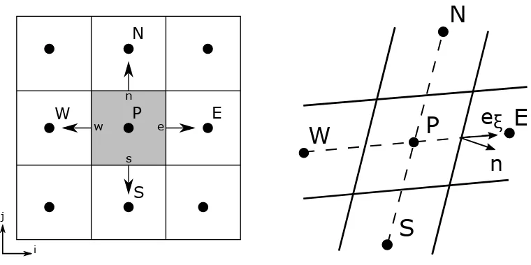
Figure 2.1: (a) A typical CV and the notation used. (b) A typical CV with a skewed

grid.

Equation (2.3) refers to the i-th Cartesian component. In Equation (2.3) and

Equation (2.4) S is the surface that bounds V, ni is the ith component of the

outward normal vector to S, and τij is the viscous stress tensor

τij =

1 Re

∂ui

∂xj

+ ∂uj

∂xi

!

. (2.5)

To obtain the previous equations we have used the Gauss theorem

Z V ∂Fi ∂xi dV = Z S

FinidS (2.6)

applied to a generic differentiable vector field Fi.

To obtain a numerical approximation to the solution of Equation (2.3) and Equation (2.4), the domain is subdivided into a finite number of contiguous, non-overlapping Control Volumes (CVs), and the conservation equations are applied to each CV, see Figure (2.1a). The method is conservative by construction, as long as the surface integrals are the same for the CVs sharing a boundary. At the centroid of each CV, we define a computational node where all the averages

of the computational variables are (ui and p) are formally assigned. Using this

2.1 Finite volume method 7

In order to numerically solve our equations, we have to introduce a

numer-ical approximation for the surface and volume integrals. Since in 3D each cell

has a cuboidal shape, the net flux through a CV boundary is the sum of the contributions over six faces

Z

S

f dS =X

k

Z

Sk

f dS, (2.7)

wheref is any component of a flux vector in the direction normal to the face (e.g.,

the normal convective or viscous flux in the momentum equations, R

SuiujnjdS

andR

SτijnjdS, respectively). Note that, for an incompressible fluid with constant

viscosity, the viscous flux reduces to

Z

S

τijnjdS =

1 Re Z S ∂ui ∂xj

njdS. (2.8)

The surface integral is approximated using the mid-point rule, leading to an approximation of second-order accuracy. In this quadrature, the integral is ap-proximated as the product of the integrand at the cell-face center and the corre-sponding surface area. As an example the flux on the east face of a rectangular cell would reads as:

Fe=

Z

Se

f dS ≈feSe. (2.9)

Equation (2.9) requires the values of the variables at the face centre. To obtain

these values, we use a linear interpolation between the two nearest nodes,fE and

fP. For example, at location e we have

fe =fEλe+fP(1−λe), (2.10)

where the linear interpolation factorλe is defined as

λe=

xe−xP

xE−xP

. (2.11)

This method is also second-order accurate and on a Cartesian mesh would cor-respond to the central-difference approximation of the first derivative in a finite difference framework. The assumption of a linear variation between points P and E, provides also a simple method to approximate the derivative,

∂f ∂x

!

e

≈ fE −fP xE −xP

. (2.12)

Some terms also require integration over a CV. To compute the integral up to second-order accuracy, the mid point rule is extended as

QP =

Z

V

Since all variables are available at the CV center, no interpolation is required. We are now able to write the full spatial approximations of Equation (2.3) and Equation (2.4). The volume integrals, corresponding to the unsteady, pressure and forcing terms, can be easily computed applying Equation (2.13). The

con-vective flux Fc _{is computed by assuming that the mass flux ˙m is already known}

using the midpoint rule approximation

F_ec =

Z

Se

uu·ndS ≈m˙eue, (2.14)

here, again for the sake of simplicity, we have considered only the x component

of the velocity field, ˙me being the mass flux on the e face, computed as

˙ me =

Z

Se

ujnjdS ≈(u·n)eSe. (2.15)

In order to compute the diffusive flux Fd

F_ed=

Z Se 1 Re ∂u ∂xj

njdS ≈

1

Re(∇u·n)eSe, (2.16)

the gradient of u at the cell face center is needed. First, we approximate the

derivative at the CV center by the average value over the cell

∂u ∂xi ! P ≈ Z V ∂u ∂xi dV VP , (2.17)

then, we apply the Gauss theorem to the numerator

Z V ∂u ∂xi dV = Z S

uei·ndS ≈

X

c

ucSci for c=e, n, w, s, b, t, (2.18)

where ei is the unit vector in the i-th direction. Finally, the derivative can be

computed as ∂u ∂xi ! P ≈ P

cucSci

VP

. (2.19)

Using interpolated cell face values to compute the derivative may generate an oscillatory solution. To solve this problem we use the so-called deferred correction method [11] as proposed by Muzaferija [69], where an additional term is added which is the difference between the correct and approximated flux. The diffusive flux is corrected as follows

F_ed=F_ed_{impl +}hF_ed_expl−F_ed_impliold, (2.20)

2.1 Finite volume method 9

When the line connecting nodes P and E is orthogonal to the cell face, the

derivative with respect toncan be approximated by a derivative with respect to

the coordinate eξ along that line, and the implicit flux is written with a second

order accurate approximation as

F_ed_{impl =} 1

ReSe ∂u ∂ξ

!

e

. (2.21)

When the grid is non-orthogonal, the deferred correction term must contain the

difference between the gradient in the n and eξ directions (see Figure (2.1b)).

So, the diffusive flux can be written as

F_ed = 1 ReSe

∂u ∂ξ

!

e

+ 1

ReSe

" ∂u ∂n ! e − ∂u ∂ξ ! e #old , (2.22)

where the first term on the right hand side is the one treated implicitly, while the second one is the deferred correction, which is calculated using interpolated cell center gradients, resulting in the following expression for the diffusive fluxes

F_ed= 1 ReSe

uE −uP

LP,E

+ 1

ReSe(∇u) old

e ·(n−eξ). (2.23)

If the line connecting nodes P and E is orthogonal to the cell face, the deferred

correction term is null as expected. Note that, this correction does not affect the second-order accuracy of the method.

2.1.1

Time discretisation

The numerical solution of the incompressible Navier-Stokes equations is com-plicated by the lack of an independent equation for the pressure. In fact, the continuity equation does not have an explicit time derivative applied to the pres-sure or to the density variable. Indeed, in incompressible flows, the continuity equation is just a kinematic constraint on the velocity field, rather than a dy-namic equation. One way to solve this problem is to rely on the fractional step method. This technique was firstly developed by Chorin [25] and later on modi-fied and improved by several other authors. The results obtained in the thesis rely on a modified version of the method originally proposed by Kim and Moin [52]. The algorithm is based on the Hodge’s decomposition of the velocity field into a solenoidal and an irrotational part, and consists of two stages: the prediction step, where the momentum equation is solved without satisfying the continuity equation, and the correction step, where the previous solution is corrected by projecting the velocity field onto a divergence-free field.

We can write the numerical discretization of the incompressible Navier-Stokes equations concisely as follows

u∗−un

∆t =−Nl

un,un−1+ 1 ReL(u

∗

un+1_−u∗

∆t =−G

φn+1, (2.25)

with the constraint

Dun+1= 0. (2.26)

u∗ is the predicted velocity field,unthe solenoidal velocity field at timen, ∆tthe

time step, Nl, G, D and L are the discrete non-linear, gradient, divergence and

Laplacian operators, respectively, and φ is the projection variable. Note that,

the operators include coefficients that are specific to the selected time scheme.

The variable φn+1 _{to be used in the projection (Equation (2.25)) can be found by}

solving a Poisson equation for φ, obtained by applying the divergence operator

to Equation (2.25), which gives

Lφn+1 = 1

∆tD(u

∗

), (2.27)

with the boundary condition

∂φn+1

∂n = 0, (2.28)

with n being the outward normal vector. So, the sequence to solve the

incom-pressible Navier-Stokes equations by a fractional step method consist of a pre-diction step (Equation (2.24)), a Poisson equation (Equation (2.27)), and a final correction step (Equation (2.25)). Computationally speaking, the most expensive step is the one related with the solution of the Poisson pressure equation. How-ever, when the span-wise direction is homogeneous, periodic boundary conditions

can be assumed and a 3D Poisson equation can be transformed into a series of

two-dimensional Helmholtz equations in wave number space via a Discrete Fast

Fourier transform (FFT). In particular, assuming z to be the periodic direction,

φ is transformed in the wave number space using the discrete anti-transform

φ(x, y, z) =

N−1

X

l=0

ˆ

φl(x, y)exp(ilz), (2.29)

where ˆφlis thelthFourier coefficient ofφandN is the number of modes considered

(i.e., l = 0, . . . , N −1). Using the orthogonality property of the Fourier system,

we obtain a set of decoupled Helmholtz equations

∂2_φˆ

l

∂x2 +

∂2_φˆ

l

∂y2 −klφˆl = ˆrl, (2.30)

wherekl is the modified wave number and ˆrl is the Fourier transform of the right

hand side of Equation (2.27). Further details can be found in [20].

2.1 Finite volume method 11

equation needs to be discretised on a grid which is coarser than the one used for the predicted variables. The mismatch in the number of discrete values makes the kernel of the pressure operator non trivial giving rise to pressure spurious modes. To eliminate those modes we use a method originally proposed by Rhie and Chow [77]. Initially, we solve the momentum equation as usual, and then (before solving the Possion equation) the mass fluxes obtained with the interpolated velocity are corrected by subtracting the difference between the pressure gradient and the interpolated gradient at the cell face location obtained at the previous time step

˙

me = (u·n)_eSe−∆tSe[(pE −pP)−∇p·eξ]old. (2.31)

This method automatically detects the oscillations and smooths them out.

2.1.2

Numerical implementation

The discrete counterparts of Equation (2.3) and Equation (2.4) have been imple-mented in a well-established curvilinear finite volume code [71, 72, 81] written in Fortran 77. As previously mentioned, the code approximates the fluxes us-ing a second-order central formulation (Figure (2.2a)), and the Rhie and Chow method [77] to avoid pressure oscillations. The equations are advanced in time by a second-order semi-implicit fractional-step procedure [52], where the implicit Crank-Nicolson scheme is used for the wall normal diffusive terms, and the ex-plicit Adams-Bashforth scheme is employed for all the other terms. The Poisson pressure equation obtained when using a pressure correction method to enforce the solenoidal condition on the velocity field is transformed into a series of two-dimensional Helmholtz equations in wave number space via Fast Fourier

trans-form (FFT) in the spanwise direction. Each of the resultant elliptic 2D problem

is then solved using a preconditioned Krylov method (PETSc library [6]). In

particular, for the problem at hand, we have found the iterative Biconjugate Gradient Stabilized (BiCGStab) method with an algebraic multigrid precondi-tioner (boomerAMG) [42] to behave quite efficiently. The code is parallelized

using the domain decomposition technique and the MPI message passing library. Figure (2.2b) shows the scalability of the code, defined as the ratio between the

time needed to perform one time-step with one processor T1 divided by the time

using n processors Tn. The test was performed with a 3D C-grid around an

aerofoil with 480×206×96 points in the x, y and z directions respectively. A

validation of the baseline code using a classical turbulent flow is given in the next section.

2.1.3

Turbulent channel flow

y

z

x

h

-h

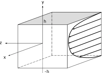
Figure 2.3: Sketch of the channel geometry.

We consider the flow of an incompressible viscous fluid through a channel with impermeable walls, as sketched in fig 2.3. We introduce the Cartesian coordinate

system shown in figure 2.3, wherex,y andz denote the stream-wise, wall-normal

and span-wise coordinates, whileu,v andwdenote the respective components of

the velocity vector field. The lower and upper walls are located aty=−handy=

h, respectively. At the walls, we impose the no-penetration and no-slip conditions.

It is assumed that the fully developed turbulent channel flow is homogeneous in the stream-wise and span-wise directions, so that periodic boundary conditions can be used in these directions. To make the problem dimensionless, we define

as a characteristic length L∗ one-half the channel

L? =h, (2.32)

and as characteristic velocity U? the bulk velocity

U? =Ub =

1 2h

Z h

−h

U dy, (2.33)

where U(y) is the mean velocity profile. With this choice, the Reynolds number

is defined as

Reb =

Ubh

2.1 Finite volume method 13

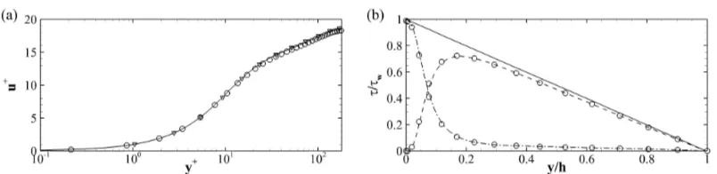
Figure 2.4: (a) Mean velocity profile in wall units. (b) The total shear stress (solid

line), decomposed in the viscous stress (dash-dotted line) and Reynolds shear stress (dashed line) obtained from from simulation. The circles in both the plots are used for the results by Kim, Moin and Moser [53], while the triangles in the fist plot are used for our result on a coarser grid.

whereνis the kinematic viscosity defined asν =µ/ρ. The bulk Reynolds number

Reb is fixed to 2800, and the computation is carried out on a grid of 256×192×192

points, in the x,y and z directions respectively. The computational domain size

is set to 2πh×2h×πhin the x,yans z directions. With the mentioned grid, the

resolution turns out to be ∆x+ ≈ 5 in wall units in the stream-wise direction,

∆z+ _{≈3 in the span-wise direction, and with a minimum ∆y}+ _{in the wall-normal}

direction which is less than 1.

The wall units, indicated by the superscript " + ", are measured in terms of

the dimensionless viscous lengthδν, which is defined as follows

δν =

1 uτRe

, (2.35)

whereuτis the dimensionless friction velocity. Note that we use the viscous length

and the friction velocity as reference length scale and velocity scale, respectively, in the near-wall regions. For a turbulent channel flow with solid walls, the friction velocity is defined as follows

uτ =

v u u t 1 Re du dy _y=−1

, (2.36)

where u is the mean velocity, y/h = −1 is the location of the wall, and the " ¯ "

indicates the average over both time and homogeneous directions, x and z. The

Reynolds number based on the friction velocity uτ and the channel semi-height

is called friction Reynolds number Reτ, and is defined as Reτ = uτh/ν. In our

case, the friction Reynolds number isReτ = 180.

Figure (2.4a) shows the mean velocity profilesu+=u/uτ versus the logarithm

of the distance from the wall ˜y = y−1 expressed in wall-units. The solid line

to the results of another simulation, on a grid with half points in each direction, which is used to assess the grid convergence of the results. The agreement is very good, even if our friction velocity is slightly underestimated.

The total shear stress τ, defined as the sum of the Reynolds shear stress u0_v0

with the viscous stress

τ = 1 Re

du dy −u

0_v0_{. (2.37)}

is given in Figure (2.4b), compared with the results by Kim, Moin and Moser [53]. As for the mean velocity profile, the agreement between our simulation and the reference data is very good.

The next section will introduce the immersed boundary method which is the technique that has been chosen to deal with the presence of complex and/or moving portions of the boundary.

2.2

Immersed Boundary Method

The Immersed Boundary Method (IBM) is a numerical technique used to simulate flow fields past bodies that do not necessarily conform with the computational grid. The pioneer of this numerical technique has been Charles Peskin that back in the seventies was able to simulate the flow of blood inside a heart [73]. As mentioned, the main feature of this method is that the numerical grid does not need to conform to the geometry of the object, which is replaced by a body force

distribution f that mimic the effect of the body on the fluid by restoring the

desired velocity boundary values on its immersed surface. The main advantage of the IBM is the simplification of the grid generation task. In fact, grid topology

and its quality are not determined by the complexity of the geometry. The

advantage of the IBM becomes quite clear for flows with moving boundaries, where the process of generating a new grid at each time step is avoided, since the grid can be kept stationary and non-deforming. A drawback of the approach is that the grid lines are not aligned with the body surface, so in order to obtain the required resolution, higher number of grid points may be required. Many IBMs have been proposed in the past. The main difference between the methods is related with the way in which the Immersed Boundary force is computed. IBMs can be grouped in two main categories, the continuous and discrete forcing ones. In the first approach the forcing is incorporated into the continuous equations before discretization, whereas in the second approach the forcing is introduced after the equations are discretized. The method that we will use belongs to the first group, and is termed as Reproducing Kernel Particle Method (RKPM) and was developed by Pinelli et al. [61, 62, 74].

Next, we explain how the equations are modified to take into account the presence of an immersed body when using the RKPM approach. Firstly, the

2.2 Immersed Boundary Method 15

markers, called Lagrangian pointsX. The latters, in general do not correspond

with the grid nodesx. To advance in time the Navier-Stokes equations, a simple

prediction step (Equation (2.24)) is performed, without taking into account the

immersed object. The obtained velocity field u∗ is then interpolated (with an

interpolator operator I) onto the embedded geometry Γ,

U∗ =I(u∗). (2.38)

The values ofU∗ are used to determine a distribution of singular forces along Γ

that restore the prescribed boundary valuesUΓ _as

F∗ = U

Γ_−U∗

∆t . (2.39)

The force field defined over Γ is then transformed into a body force distribution

applied to the fluid grid using a convolution operatorC

f∗ =C(F∗). (2.40)

The momentum conservation equation is then solved again with the computed volume force field added as a source term

u∗−un

∆t =−Nl

un,un−1+ 1 ReL(u

∗

,un)− G(φn) +f∗. (2.41)

Finally, the time advancement step can be completed with the usual solution of the pressure Poisson equation and the projection step. The given procedure is common to a number of IB methods. The step that define the present method

concern the way in which the operatorsI and C are built.

2.2.1

Interpolation and convolution

We use the Reproducing Kernel Particle Method (RKPM) [61, 62, 101, 74] to define interpolation and spreading operators. In this method the approximation

fa(x) of the value of a given smooth function at pointx∈Ω can be expressed as

a kernel approximation

fa(x) =

Z

Ω

wδ(x−s)f(s)ds, (2.42)

wherewδ is a non-negative kernel function of compact support, and the subscript

indicates that the kernel depends on a parameter δ, called dilation parameter,

which determines the dimension of the support ΩI. So, wδ is non-zero only in a

sub-domain ΩI of Ω and zero elsewhere. A discrete approximation of the kernel

Figure 2.5: (a) Kernel function proposed by Roma et al. [79]. (b) The black rectangle

is the cage around one of the Lagrangian points, shown as dots. The squares represents grid points, and the black ones are the grid points falling within the cage.

wδ(r) =

           1 6

5−3|r| −q−3 (1− |r|)2+ 1

, if 0.5≤ |r| ≤1.5,

1 3

1 +√−3r2_{+ 1, if 0.0≤ |r| ≤1.5,}

0, otherwise,

(2.43)

where r= (x−s)/δ. This approximation of wδ satisfies the following properties

1. wδ(r) is continuous;

2. wδ(r) = 0 if |r|>1.5;

3. P

lwδ(r−l) = 1;

4. P

l(r−l)wδ(r−l) = 0;

5. P

l[wδ(r−l)]

2

= 1/2.

In the the last three properties, the sums are performed ∀l∈_N, and are satisfied

∀r ∈_R. For example, forr = 0.0, the functionwdis not null forl =−1,0,1 where

it is equal to 1₆,2₃,1₆ (see the dots in Figure (2.5a)). Since the previous properties

involve the natural number l, they can be satisfied by a function interpolated

using Equation (2.42) and Equation (2.43) only if the nodes are equispaced. To extend this approach to a non-uniform nodes distribution, following Liu et al.

[62] and Pinelli et al. [74], we use a modified window function weδ, defined as

e

wδ(x−s) = n

X

i=0

bi(x−s)iwδ(x−s), (2.44)

where bi are n+ 1 coefficients determined by imposing the continuous equivalent

of properties 3 and 4, which are

f

mi(x) =

Z

Ω

2.2 Immersed Boundary Method 17

where δij is the Kronecker’s delta. Note that, these conditions imply the exact

representation of the elements of the canonical polynomial base {1, x, x2_{, . . .}.}

The number n is the higher order of the polynomial that we want to represent

exactly. For example,n = 2 would lead to an exact representation of all

polyno-mials of degree up to 2. Substituting Equation (2.44) into Equation (2.45), we obtain

f

mi(x) =

Z

Ω

(x−s)iweδ(x−s)ds=

n

X

j=0

bjmi+j(x) =δi0, (2.46)

fori= 0,1, . . . , n, where we have defined

mi(x) =

Z

Ω

(x−s)iwδ(x−s)ds. (2.47)

The above equations form a symmetric linear system M~b =~e1, where the right

hand side~e1 is a vector, whose elements are all zeros, except the first one which

is equal to 1. From the solution of this linear system (Equation (2.46)) we can

obtain the coefficientsbi, and, finally, we can write the corrected window function

(here given forn = 2) as

e

wδ(x−s) = [bo+ (x−s)b1+ (x−s) 2

b2]wδ(x−s). (2.48)

The procedure can be extended to higher dimensions, defining the window

function as a Cartesian product of the 1Dkernels. In 2D, it becomes

wδ,η(x−s, y−t) =wδ(x−s)wη(y−t) (2.49)

and in 3D

wδ,η,σ(x−s, y−t, z−v) =wδ(x−s)wη(y−t)wσ(z−v), (2.50)

whereδ,ηandσ are the dilatation parameters in the coordinates directions. The

linear systems to find the coefficientsbi,j andbi,j,k are obtained from the following

conditions

f

mi,j =

Z

Ω

(x−s)i(y−t)jweδ,ηds =δl0 for i, j = 0,1, . . . , n, (2.51)

in 2D, wherel =i+j and i+j ≤n, and

f

mi,j,k =

Z

Ω

(x−s)i(y−t)j(z−t)kweδ,η,σds =δl0 for i, j, k = 0,1, . . . , n, (2.52)

in 3D, wherel =i+j+k and i+j+k≤n. So, the corrected window functions

in 2D and 3D are

e

wδ,η(x−s, y−t) = [b0,0+ (x−s)b1,0+ (y−t)b0,1+

(x−s) (y−t)b1,1+ (x−s) 2

b2,0+ (y−t) 2

b0,2]×

wδ,η(x−s, y−t),

and

e

wδ,η,σ(x−s, y−t, z−v) = [b0,0,0+ (x−s)b1,0,0+ (y−t)b0,1,0+ (z−v)b0,0,1+

(x−s) (y−t)b1,1,0+ (y−t) (z−v)b0,1,1+ (z−v) (x−s)b1,0,1+

(x−s)2b2,0,0+ (y−t) 2

b0,2,0 + (z−v) 2

b0,0,2]×

wδ,η,σ(x−s, y−t, z−v),

(2.54)

respectively.

Finally, we briefly describe the implementation of the IB based on RKPM.

Around each Lagrangian node X we define a cage that contains at least three

nodes of the underlying mesh in each direction, as shown in Figure (2.5b), whose

edges measure 3δ, 3η and 3σ in x, y and z, respectively. After finding the

set of mesh nodes that fall within the cage, the terms of the moment matrix (Equation (2.52)) can be numerically evaluated to assemble the local window

function, using the mid-point quadrature rule. The coefficients~bof the correction

polynomials are found by solving the symmetric linear system M~b=~e1 for each

Lagrangian points. Due to the very low values that the window function may take at the nodes close to the boundary of the cage, the moment matrix may become ill conditioned. This problem is avoided by rescaling the linear system,

and solving the equivalent one HM H−1~b_=~e

1, where the diagonal matrixH has

the inverse of the dilation factors in the main diagonal. In 3D H is

H = diag 1,1

δ, 1 η, 1 σ, 1 δη, 1 ησ, 1 δσ, 1 δ2,

1 η2,

1 σ2

!

. (2.55)

Once the coefficientsbhave been found, the window functionweδ,η,σ can be used for

the interpolation (Equation (2.38)) and spreading (Equation (2.38)) operations. In particular, the discrete interpolation, using a mid point rule becomes

Ul =I(ui,j,k) =

X

i,j,k∈ΩI

ui,j,kw˜δ,η,σ(xi,j,k−Xl) ∆Vi,j,k, (2.56)

while the spreading operation reads

fi,j,k =C(Fl) = N

X

l=1

Flw˜δ,η,σ(xi,j,k−Xl)l, (2.57)

where l is a characteristic volume related to the local dilation coefficients of the

window function. To determine the correct value of, first, we consider the value

of the force on the Lagrangian points, obtained by interpolation

Fl =

X

i,j,k∈ΩI

2.2 Immersed Boundary Method 19

then, we replace fi,j,k with Equation (2.57)

Fl=

X

i,j,k∈ΩI

"_N X

l=1

Fmw˜δ,η,σ(xi,j,k−Xm)m

#

˜

wδ,η,σ(xi,j,k −Xl) ∆Vi,j,k. (2.59)

Equation (2.59) can be written using a matrix notation as

Adiag (~)F~ =F .~ (2.60)

By requiring that~is independent of the actual force distribution, we obtain the

constraint det [Adiag (~)] = 0, whose solution is found by solving

A~=~1, (2.61)

where~1 is a vector, whose elements are all ones. As shown by Pinelli et al. [74],

the conditioning of the matrixA depends on the ratios between the distances of

the Lagrangian nodes and the local grid size. When the Lagrangian spacing is approximately equal to the local grid size (or slightly higher), the linear system

for~is well conditioned and is easily solved.

2.2.2

Flow around a cylinder

y

x D

20D 20D

10D 30D

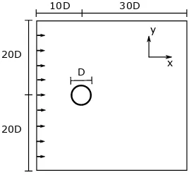
Figure 2.6: Sketch of the computational domain around a cylinder.

To validate the RKPM immersed boundary implementation, we consider the flow of an incompressible viscous fluid around a circular cylinder, as sketched in Figure (2.6). We introduce the Cartesian coordinate system shown in Figure (2.6),

wherexandy denote the stream-wise and normal coordinates, whileuandv

stream-wise direction U∞ is imposed at the inlet of the domain, while a convec-tive outlet condition is imposed at the outlet. To make the problem dimensionless,

we use as a characteristic length L∗ the cylinder diameter

L∗ =D, (2.62)

and as characteristic velocity U∗ the free-stream velocity

U∗ =U∞. (2.63)

Consistently, the Reynolds number is defined as

ReD =

U∞D

ν . (2.64)

The diameter Reynolds number is fixed to ReD = 100, and the computation is

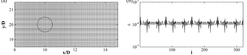
Figure 2.7: (a) Grid in the proximity of the cylinder (nodes are plotted with a skip index of 5). (b) The values of for every Lagrangian points.

carried out on a grid of 696×696 points, covering a computational domain of

40D×40D. The center of the cylinder is located at (10D,20D), and its surface

is discretised with 320 equispaced Lagrangian points. The grid has an uniform

spacing of 0.001 in the cylinder region, and stretches towards the boundaries of

the domain. Note that, grid points are present also inside the cylinder, as shown

in Figure (2.7b). Figure (2.7b) reports the values of for all the Lagrangian

points. Note that, the square root of the average value 0.00011 is approximately

equal to the mesh size.

Figure (2.8a) shows the instantaneous span-wise vorticity ωz fields around

the cylinder. At this Reynolds number, the wake of the cylinder is

charac-terised by a von Karman vortex street typical of bluff bodies. Vortices of op-posite sign are shed from the cylinder periodically, at a Strouhal number equal

to St = fsD/U∞ = 0.17, which is close to the experimental value of St = 0.165

reported by Williamson [97]. The value was obtained by the spectrum of the in-stantaneous lift coefficient value, whose time history is reported in Figure (2.8b) with a solid line together with the drag coefficient shown with a dashed line. The

2.2 Immersed Boundary Method 21

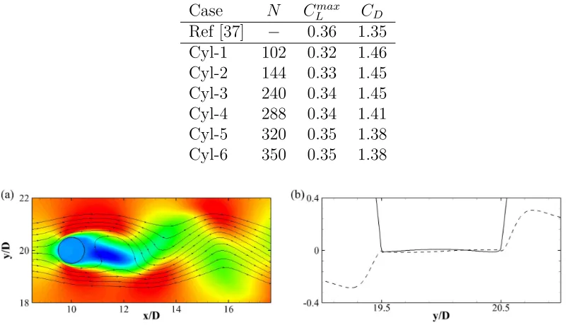
Figure 2.8: (a) Contours of the span-wise vorticity ωz. (b) Evolution of the liftCL

(blue) and drag coefficientsCD (red) over time.

Table 2.1: Aerodynamic coefficients for the cases analysed. The data from the first

row are taken from Guilmineau and Queutey [37].

Case N Cmax

L CD

Ref [37] − 0.36 1.35

Cyl-1 102 0.32 1.46

Cyl-2 144 0.33 1.45

Cyl-3 240 0.34 1.45

Cyl-4 288 0.34 1.41

Cyl-5 320 0.35 1.38

Cyl-6 350 0.35 1.38

Figure 2.9: (a) Contours of the stream-wise velocity u. (b) u (solid line) and v

(dashed line) velocity profiles, coloured in red and blue, respectively, atx= 10D.

the maximum absolute lift value equal toCmax

L = 0.35. These results are in good

agreement with the one obtained by Guilmineau and Queutey [37] who found a

mean drag coefficient CD = 1.35, and a maximum lift equal to CLmax = 0.36.

Table (2.1) reports the mean drag coefficients CD and the maximum

instan-taneous lift coefficients Cmax

L obtained from various simulations, changing the

number of Lagrangian points used to represent the cylinder surface. We notice that the cases with 320 and 350 points have the same values, thus indicating that 320 points is enough to correctly represent the solid cylinder at this Reynolds number.

U∞

α

outlet

inlet

Figure 2.10: Sketch of the computational domain.

the cylinder. In Figure (2.9b) theuandv velocity profiles on a vertical line

pass-ing through the centre of the cylinder at x = 10D are reported using solid and

dashed lines, respectively. Both the velocity components have values close to 0 at the cylinder boundary, and small but non zero values inside the cylinder, a typical situation encountered when using IB methods.

2.3

Flow around aerofoils

We now briefly describe the numerical set-up that has been used as a common ground to simulate the flow around an infinite NACA0020 wing. In particular, we will introduce the grid system, the boundary conditions, and the technique used to keep into account the aerofoil rotation. This section finalizes with the description of a test case used to validate the numerical implementation used for the DNS of the flow around aerofoils.

2.3.1

Numerical set-up

We now consider an incompressible three-dimensional unsteady flow field around

a straight wing with an infinite span-wise dimension z (x3). The computational

domain is shown in Figure (2.10). The coordinate system is Cartesian with thex

and yaxis (x1 and x2) denoting the directions parallel and normal to the aerofoil

chord, respectively. Also, u, v and w (u1, u2 and u3) denote the correspondent

components of the velocity vector field parallel and normal to the chord, and

along the span. The Reynolds number Rec = U∞c/ν is based on the chord

length of the aerofoil cand the approaching free-stream velocity magnitude U∞.

We use U∞ and cas the velocity and length scales for normalisation throughout

the rest of the thesis.

2.3 Flow around aerofoils 23

is obtained by repeating the baseline 2D grid uniformly in the spanwise

direc-tion. With this arrangement, the external surface that bounds the computational domain, contains both the inlet and the outlet (see Figure (2.10)). To determine

which portion of the boundary in all parallel x-y planes is either an inlet or an

outlet, at each time step a local spanwise average of the fluid velocity is evaluated in a tiny region close to the boundary. When the averaged flow direction points outward, the corresponding portion of the boundary is assumed to be an outlet, and is treated using a convective boundary condition. Conversely, if the flow direction is directed inward, the corresponding boundary surface is considered to be an inlet, and a Dirichlet type condition based on an irrotational approxi-mation is employed. In particular, the values to be assigned to the velocity on the Dirichlet portions of the boundary are determined by solving a companion potential equation discretised via a Hess-Smith panel method [43].

Finally the remaining boundary conditions are imposed by enforcing: imper-meability and no slip conditions on the aerofoil wall, periodic conditions on the planes bounding the domain in the spanwise direction, and continuity of the flow variables through the symmetry plane generated by the C-grid shape downstream of the trailing edge.

2.3.2

Aerofoil rotation

When considering an aerofoil undergoing a time variation in its angle of incidence, one can consider a frame of reference mounted on the aerofoil. In particular, the

frame shown in 2.10, is a non-inertial one, which rotates around thez-axis, having

its centre of rotation located at a quarter of the chord (xo _{= 0.25c). We define}

the angle of rotation between the two reference axis as θ = −α. The

Navier-Stokes equations (Equation (2.1) and Equation (2.2)) in a non-inertial frame of reference are modified as follows,

∂ui

∂t + ∂uiuj

∂xj

=−∂p

∂xi

+ 1

Re ∂2_u

i

∂xj∂xj

+θI¨ _ijθxj + 2 ˙θIijθuj + ˙θ2xi

, (2.65)

∂ui

∂xi

= 0. (2.66)

where all the variables are evaluated in the non-inertial frame of reference, and the terms in the brackets are the inertial forces. In particular, the three terms are

the Euler, the Coriolis, and the centrifugal forces, respectively. Iθ is an auxiliary

matrix defined as

Iθ =



 

0 1 0

−1 0 0

0 0 1





. (2.67)

The boundary condition are modified as well. In particular, a Dirichlet condition becomes

Figure 2.11: LiftCL(blue) and dragCD (red) coefficients as a function of time. The

solid line is used for the case with inertial forces, while the dashed line for the case without. The green line represents the time variation of the angle of attack.

wherevi is the Dirichlet value for the velocity in the inertial frame, and Rθ is the

rotation matrix

R_ijθ =

  

cos (θ) sin (θ) 0

−sin (θ) cos (θ) 0

0 0 1

 

, (2.69)

while the Neumann condition for the Poisson equation remains unchanged. To

avoid numerical oscillations the function θ =θ(t) has been made continuous up

to its second derivative, thus, we use a ramp function with smoothed start and finish.

An alternative, simplified approach to represent the time variation of the angle of attack is to modify the Dirichlet inlet conditions in time. At each time step, the velocity components are modified to keep into account the change in the direction of the freestream velocity vector. This method does not reproduce standard wind tunnel experiments where the aerofoil is rotated around a revolution axis.

However, for low values of ˙θ and ¨θ, the two approaches lead to similar results in

terms of integral quantities, with some discrepancy in the shape and evolution of the wake (see Wong et al. [98]). In the ramp-up manoeuvre that will be analysed,

we will consider ˙θ as a constant except in short periods of time at the beginning

and at the end of the manoeuvre, when ¨θ is adjusted to enforce a smooth time

variation of θ. In Figure (2.11), we compare the lift and drag time history using

the two described approaches, using a value of ˙θc/U∞ = 0.12. In the graph, the

2.3 Flow around aerofoils 25

Table 2.2: Aerodynamic coefficients, separation and reattachment points for a

NACA0012 at α = 5o and α = 8o (Rec = 50000). The first two rows values are

from Lehmkuhl et al. [59], the second two correspond to our predictions.

Case α CL CD xs/c xr/c

Val-5-Ref 5o _{0.57 0.029 0.065 0.57}

Val-8-Ref 8o 0.76 0.050 0.024 0.32

Val-5 5o _{0.57 0.028 0.100 0.57}

Val-8 8o 0.73 0.049 0.032 0.30

2.3.3

Flow around an aerofoil: validation

The baseline code used for this thesis has been extensively validated for various turbulent flows in the past [70, 71, 72]. However, to further corroborate the predictive capabilities of the code in aeronautical contexts, we report a specific validation of the flow over a NACA0012 aerofoil. We compare our numerical results with the ones obtained by Lehmkuhl et al. [59] and by Rodriguez et al. [78]. In particular, we have considered the aerofoil at a chord Reynolds number

Rec= 5×104, and at angles of attackα= 5oandα = 8o. The simulation domain

has been set up and discretised as previously described. We have used a grid of

2545×490×48 points in thex1, x2 and x3 directions, with a reduced spanwise

extent of the domain (set to 0.2c, as in [78]).

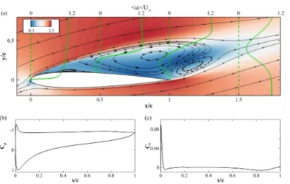
The comparison with the reference data turns out to be quite satisfactory. In particular, Figure (2.12a) shows the pressure coefficient distribution over the aerofoil surface at the two angles of attack obtained in the present simulations versus the ones given in [59]. At both angles of attack all the predictions show the presence of a separation bubble on the suction side of the aerofoil, resulting in

a plateau in the pressure coefficient. At α = 5o _{the flow separates at x}

s ≈0.10c

and reattaches atxr≈0.57c, while atα= 8o the separation occurs atxs≈0.03c

and the reattachment at xr≈0.30c. A quantitative comparison with the results

by Lehmkuhl et al. [59] is given in Table (2.2). In general, we find an overall good agreement with the reference results, with a slightly retarded separation

predicted by our simulations. Figure (2.12b) shows the mean x-velocity profiles

in the vicinity of the trailing-edge and in the near wake region atα = 8o. Again,

Chapter 3

Flow around an aerofoil in static

and dynamic stall

3.1

Introduction

The flow around aerofoil at high angle of attack in full stalled condition is a problem of great interest in aerodynamics and fluid-dynamics, since it involves separation of the flow from the leading edge, transition to turbulence in the sep-arated shear layer and the shedding of vortices in the wake, the latter being responsible of strong fluctuation in the lift and drag. The static stall of aerofoil can be classified into three basic types [48, 65]: i) trailing-edge stall, when the separation starts from the trailing edge and moves forward with increasing angle of attack, ii) leading-edge stall, which results from the burst of laminar separation bubble, and iii) thin-aerofoil stall, characterised by flow separation at the leading edge with reattachment in a point which moves progressively downstream with increasing angle of attack. Note that, the aerofoil stall type depends on several variables (Reynolds number, surface roughness or free-stream turbulence), there-fore, its stall type may change when flow conditions are changed. Broeren and Bragg [15] showed that the most severe unsteady effects are those encountered in the thin-aerofoil and trailing-edge stall type.

on the helicopter blades the objective is mainly to inhibit the formation of the dynamic stall vortex, on fixed wing aircraft, the idea could be to sustain the lift overshoot generated by the dynamic stall vortex formation to enhance the manoeuvrability.

So far, experimental works have mainly focused on unsteady flows over two-dimensional aerofoils undergoing prescribed pitching motions [38, 28, 29, 30, 31, 63, 64, 57, 67, 68]. Most of these works [38, 28, 29, 30, 31, 63, 64] have also investigated the influence on the aerodynamic response of various parameters, such as aerofoil geometry, Reynolds and Mach numbers, oscillation amplitude and frequency. Halfman et al. [38] created a combined experimental and theoretical method able to predict the effect of the dynamic stall on the aerodynamic load. This approach was further developed by Ericsson and Reding [28, 29, 30, 31]. McCroskey [63, 64] described the main physical features of the phenomenon and classified the dynamic stall into two categories: light and deep stall, the former being characterised by a loss of lift and an increase in drag which are of the same magnitude as the one associated with the classical static stall, and by a size of the separated region in the order of the aerofoil thickness. Conversely, deep stall is characterised by a lift overshoot, due to the passage of a large scale vortex over the suction side of the aerofoil, followed by a lift breakdown associated with the vortex detachment. Deep stall is also characterised by a separated region with a size in the order of the aerofoil chord. Shih et al. [87], using particle image velocimetry visualisations, suggested that the main stall vortex is induced by the early boundary layer separation near the leading-edge of the aerofoil, and that full stall occurs when the boundary layer detaches completely from the aerofoil. Acharya and Metwally [2] have highlighted the presence of two pressure peaks in the forward portion of the aerofoil. The first suction peak grows in magnitude as the aerofoil pitches up, while the second one corresponds to the dynamic stall vortex and moves downstream.

High fidelity numerical simulations of dynamic stall in configuration of aero-nautical interest are particularly expensive due to the broad range of time and space scales involved in the phenomenon: the unsteady variations of the angle of attack becomes slower and slower compared to the fastest turbulence time scale as the Reynolds number is increased. For this reasons Direct and Large Eddy Simulations (DNS and LES) are confined to low/intermediate Reynolds numbers while higher Reynolds Simulations are normally dealt with Reynolds-Averaged Navier-Stokes simulations (RANS). However, conventional turbulence models are known to fail in producing reliable solutions in such complex, out of equilibrium conditions: unsteady, recirculating and locally transitional flow.

3.2 Set-up 29

dynamic stall. In particular, Wang et al. [96] used two variants of thek−ωmodel,

the standard and the SST one, to simulate the flow at moderate high Reynolds

number Rec = 105. From a comparison with experimental results, they noticed

that the models can not precisely capture the size and position of the dynamic stall vortex. Moreover, the quality of the predictions of the models deteriorate as the angle of attack increases. Dumlupinar and Murthy [26] further investigated the performances of various turbulence models and pointed out that different turbulence closures predict a broad range of different behaviours even in the light stall case.

Although several experimental and numerical studies have contributed in elu-cidating the main physical mechanism that come into play on the flow behaviour when the angle of attack undergoes a dynamic change, to our knowledge the only high fidelity numerical simulations (i.e., DNS or resolved LES) which have been carried out so far are the implicit Large Eddy Simulations of a pitching aero-foil undertaken by Visbal [93, 94]. Those simulations can be considered to be a pioneering work aimed towards a more detailed understanding of the physical mechanisms that determine the dynamic stall vortex creation and its detach-ment. The understanding of this basic phenomenon would enable to devise new strategies and devices to control the changes in the aerodynamic loads. In this work, for the very first time we aim at performing a direct numerical simulation of the transitional flow around an aerofoil in ramp-up motion. In a companion simulation we also study the flow in a fully separated condition (at the same max-imum angle of attack) to establish a baseline benchmark case to allow a cross comparison between the aerodynamic behaviour in a static and dynamic stalled condition.

3.2

Set-up

The aerofoil that has been selected for the present study is a symmetric NACA0020. All the simulations have been undertaken by fixing the Reynolds number based on the magnitude of the freestream velocity and the chord length to 20000. The

angle of attack is kept at 20o _{in the static case, and varies according to a ramp}

function in the dynamic case. In the latter, the angle of attack is varied at a

con-stant rate equal to ˙α= 0.12U∞/c until a maximum incidence of 20o is achieved.

We now give more details on the grid system. The mesh in Figure (3.1)

has been generated in thexy-plane with particular care to its orthogonality and

stretching features using the commercial software Pointwise [75], with hyper-bolic PDE extrusion methods. The resulting grid has a minimum included angle

(83.19o) exactly matching the geometrical constraint of the trailing edge, see

Figure (3.1), while the average grid included angle in all the domain is equal to

89.97. In the wall normal direction, the grid is almost uniform from the aerofoil

Figure 3.1: Grid in the proximity of the aerofoil (nodes are plotted with a skip index of six). The inserted figure is an enlargement of the area surrounding the trailing edge.

Figure 3.2: Mean streamwise velocity< u >(a) and shear component of the Reynolds

sress tensor < u0v0 > (b) profiles over the wing and in the near wake. The solid lines are used for the reference grid, the circles and the triangles for the coarse and fine grids, respectively.

at high Reynolds number. Further away from the surface, it is coarsened with an increasing stretching factor, which maximum is located near the external

bound-ary where it is equal to 1.03. In the direction parallel to the aerofoil, the grid

is uniform over the wing and very slightly stretched (1.001) in the wake region.

A buffer layer with higher stretching factor (1.015) is used near the outlet to

suppress reflections. The three dimensional mesh is then obtained by repeating the two dimension grid in the spanwise direction with uniform spacing.

The grid density has been tuned by considering a number of preliminary two and three dimensional simulations. The former allowed us to establish the grid spacing requirements in the laminar portion of the flow featuring separation and convective instabilities. The latter was used to determine the grid reso-lution requirements in the turbulent flow regions. Through these preliminary simulations, undertaken at various incidence angles, we have found that a grid

with 2785 ×626 × 97 nodes in the x1, x2 and x3 direction (−2c < x1 < 8c,