City, University of London Institutional Repository
Citation
: Blake, D., Caulfield, T., Ioannidis, C. and Tonks, I. (2014). Improved inference in
the evaluation of mutual fund performance using panel bootstrap methods. Journal of Econometrics, 183(2), pp. 202-210. doi: 10.1016/j.jeconom.2014.05.010This is the accepted version of the paper.
This version of the publication may differ from the final published
version.
Permanent repository link:
http://openaccess.city.ac.uk/6843/Link to published version
: http://dx.doi.org/10.1016/j.jeconom.2014.05.010
Copyright and reuse:
City Research Online aims to make research
outputs of City, University of London available to a wider audience.
Copyright and Moral Rights remain with the author(s) and/or copyright
holders. URLs from City Research Online may be freely distributed and
linked to.
City Research Online: http://openaccess.city.ac.uk/ [email protected]
DISCUSSION PAPER PI-1405
Improved Inference in the Evaluation of
Mutual Fund Performance using Panel
Bootstrap Methods
David Blake, Tristan Caulfield, Christos Ioannidis
and Ian Tonks
June 2014
ISSN 1367-580X
The Pensions Institute
Cass Business School
City University London
106 Bunhill Row
London EC1Y 8TZ
UNITED KINGDOM
Improved Inference in the Evaluation of Mutual Fund Performance using Panel Bootstrap Methods
By
David Blake*
Tristan Caulfield**
Christos Ioannidis***
and
Ian Tonks****
June 2014
Abstract
Two new methodologies are introduced to improve inference in the evaluation of mutual fund performance against benchmarks. First, the benchmark models are estimated using panel methods with both fund and time effects. Second, the non-normality of individual mutual fund returns is accounted for by using panel bootstrap methods. We also augment the standard benchmark factors with fund-specific characteristics, such as fund size. Using a dataset of UK equity mutual fund returns, we find that fund size has a negative effect on the average fund manager’s benchmark-adjusted performance. Further, when we allow for time effects and the non-normality of fund returns, we find that there is no evidence that even the best performing fund managers can significantly out-perform the augmented benchmarks after fund management charges are taken into account.
Keywords: mutual funds, unit trusts, open-ended investment companies, performance measurement, factor benchmark models, panel methods, bootstrap methods
JEL: C15, C58, G11, G23
* Pensions Institute, Cass Business School, City University London; ** University College London; *** Department of Economics, University of Bath; **** School of Management, University of Bath
1. Introduction
Evidence collected over an extended period on the performance of (open-ended) mutual
funds in the US (Jensen, 1968; Malkiel, 1995; Barras, Scaillet and Wermers, 2010) and unit
trusts and open-ended investment companies (OEICs) in the UK (Blake and Timmermann,
1998; Cuthbertson, Nitzsche and O'Sullivan, 2008) has found that, on average, a fund
manager cannot outperform the market benchmark and that any outperformance is more
likely to be due to “luck” rather than “skill”. The standard approach for evaluating fund
manager performance is to test it against an appropriate factor benchmark model and assess
the significance of the abnormal returns from this model (Carhart, 1997). Recent evidence in
Chen, Hong, Huang and Kubik (2004) (hereafter CHHK) finds that fund size has a negative
effect on performance due to diseconomies of scale at the fund level (in line with Berk and
Green, 2004). CHHK’s analysis applies the Fama and MacBeth (1973) method of estimating
a series of cross-sectional regressions (one for each time period), averaging the estimated
coefficients and testing for significance using the time-series variation in these estimates.
However, Petersen (2009) has shown that this methodology yields downward biased standard
errors in the presence of fund effects. He explains how to estimate standard errors in the
presence of both fund and time effects: either parametrically by including a time dummy for
each period, and then clustering standard errors by fund; or non-parametrically by clustering
on fund and time simultaneously.1 Kosowski, Timmermann, Wermers and White (2006, hereafter KTWW) have argued that it is necessary to assess the statistical significance of fund
manager performance using bootstrap methods, since the returns of individual mutual funds
typically exhibit non-normal distributions (see also Fama and French, 2010, hereafter FF).
In this paper, we will assess the performance of a panel of mutual funds, allowing for the role
of fund-specific characteristics, such as fund size, fund charges, and fund family membership.
We estimate a panel model using fixed effects and time dummies with standard errors
clustered by fund. In addition, acknowledging that fund returns are not normally distributed,
we generate a series of (non-parametric and parametric) bootstrap returns from the
benchmark models to allow for appropriate statistical inference in the presence of non-normal
fund returns.
1 Standard errors have been correctly computed in the econometrics literature for decades under different
The structure of the paper is as follows. Section 2 reviews the existing approaches to
measuring mutual fund performance and shows how these approaches can be improved using
bootstrap methods in a panel framework. Section 3 discusses the dataset we will be using.
The results are presented in Section 4, while Section 5 concludes.
2. Measuring mutual fund performance
2.1 Measuring performance using alternative benchmark models
Building on Jensen (1968), the standard framework for assessing the performance of the
manager of mutual fund i is to compare the excess returns (Ritrft) (where rft is the risk-free
rate)obtained in period t with a four-factor benchmark model (Carhart, 1997):
+it t i i mt t i t i t i t it
R rf R rf SMB HML MOM (2.1)
where the four common risk factors are the excess return on the market index (Rmt rft), the
returns on a size factor,SMBt, a book-to-market factor, HMLt (Fama and French, 1993), and
a momentum factor,MOMt (Carhart, 1997). The idea behind (2.1) is that there are certain
common factors that are known to influence returns and that the effect of these should be
excluded from any measure of a fund manager’s performance. The genuine “skill” of the
fund manager, controlling for these common factors, is measured by alpha (αi) which is also
known as the “selectivity skill”.2 Under the null hypothesis of no abnormal performance (i.e., no selectivity skill), the estimated ˆi coefficient should be equal to zero. For each fund, we
could test the significance of each ˆi as a measure of that fund’s abnormal performance
relative to its standard error; and we could also test the significance of the average value of
the alpha across the N funds in the sample (Malkiel, 1995).
However, there are a number of problems with the standard framework. First, it is potentially
incomplete since it excludes fund-specific variables which might influence performance.
2
Second, it is based on single equation estimation and ignores the panel nature of the dataset
which comprises a group of competing fund managers. The final problem is that it fails to
take adequate account of the distributional properties of the error term, it , which are
unknown, but unlikely to be normal.
With respect to the first problem, a number of other variables have also been shown to affect
mutual fund performance. CCHK and Yan (2008) establish an inverse relationship between
mutual fund size and performance: small funds outperform large funds, and this provides
support for the Berk and Green (2004) hypothesis that fund inflows degrade the performance
of the fund management team, conditional on the chosen benchmark. In respect of the
characteristics of the individual managers, Chevalier and Ellison (1999a) report that the
education level of the fund manager, as measured by the quality of the university that the
fund manager attended, affects cross-sectional differences in performance. They also show
that other individual fund manager characteristics affect the fund’s asset allocation strategies
which, in turn, determine performance. Khorana (1996) and Chevalier and Ellison (1999b)
document an inverse relationship between fund performance and manager changes. Star fund
managers can extract a larger share of the higher fee income by either moving to a larger fund
within the same organization or to another fund family (Chen, Hong, Jiang and Kubik, 2013).
Network and spillover effects have been shown to be important determinants of mutual fund
returns (Nanda, Wang and Zheng, 2004; Hong, Kubik and Stein, 2005; Cohen, Frazzini and
Malloy, 2008). Extreme examples of such networks are fund families, where a group of
mutual funds are all owned by the same management firm. Massa (2003) shows that
alternative investment strategies of mutual funds within the same family are a form of
product differentiation, and that the degree of product differentiation negatively affects
performance.
Our dataset contains a number of fund-specific variables. Based on the arguments above, we
are able to test whether the performance of a fund is, in addition to the standard common
factors, influenced by certain fund-specific factors, namely the natural logarithm of the
relative size of assets under management (lnAUM),3 the bid-ask spread (Spread),4 the natural logarithm of the relative size of assets under management of the corresponding fund family
3 The relative size is defined as the ratio of the fund’s assets under management to the average value of assets
under management across all funds in the same month.
4 The difference between the buy-price and the sell-price for the fund which is a measure of liquidity (Sirri and
(lnFAUM),5 and by the average management charge of the fund family (FMC).6 We augment the regression equation (2.1) to include these fund-specific variables.
With respect to the second problem, the standard approach estimates equation (2.1) over time
for each fund separately, resulting in no allowance being made for any common time effects
across funds, on the grounds that the four-factor model adequately captures the systematic
components of fund returns. However, if the four-factor model is mis-specified or
incomplete, there may be common time effects across funds in the sample, which could be
captured using time dummies. One way to allow for any common dependence across time of
the funds in the sample is to follow Blake and Timmermann (1998) (and also Fama and
French, 2010, Table II) and regress an equal-weighted (or a value-weighted) portfolio p of the
excess returns (Rpt rft)on the N funds on the four factors in (2.1) and test the significance
of the estimated ˆp in this regression. But such a portfolio approach does not fully exploit
the panel nature of the dataset. An improved approach is therefore to estimate equation (2.1)
(or its augmented form with additional fund-specific characteristics) in a fixed-effects panel
regression with time dummies and standard errors clustered by fund.
Our augmented model in vector notation is:
/ /
it t i t t it it
R rf x w (2.2)
where i i is the average “skill” level across all funds and time ( ) plus the
additional fund-specific “skill” level (i), tis a time effect,
7
and
5
The relative size is defined as the ratio of the fund family’s assets under management to the average value of assets under management across all fund families in the same month.
6 These fund family variables will indirectly pick up network effects and also whether better qualified managers
are employed by large fund families.
7
The time effects are measured by time dummies defined to sum to zero across all time periods. The dummies are also bi-monthly rather than monthly on account of a very high degree of multicollinearity we encountered
/
/
/
/
( , , , )
( , , , )
(ln , , ln , )
( , , , )
t mt t t t t
it it it ft ft
x R rf SMB HML MOM
z AUM Spread FAUM FMC
CCHK do not report estimates based on the specification (2.2). Instead, they use a two-stage
estimation process. At the first stage, (2.1) is estimated for each fund separately and abnormal
returns are defined as:
/ˆ ˆ
it it it t t i
FUNDRET R rf x (2.3)
At the second stage, the following model is estimated (where we have added time effects to the CCHK specification):
/
it i t it it
FUNDRET w (2.4)
We also report results from this two-stage process.
The final problem with the standard approach that needs to be addressed is the non-normality
of returns. KTWW (p.2559) put this down to the possibilities that (1) the residuals of fund
returns are not drawn from a multivariate normal distribution, (2) correlations in these
residuals are non-zero, (3) funds have different risk levels, and (4) parameter estimation error
results in the standard critical values of the normal distribution being inappropriate in the
cross section. The solution is to use bootstrap methods to derive more accurate confidence
intervals and hence improve inference.
2.2 Measuring performance using bootstrap methods
The non-parametric bootstrap
On account of non-normalities in fund returns, bootstrap methods can be applied to the
standard benchmark model (2.1) and the augmented model (2.2) or (2.4) to assess
preserve the cross-correlation of returns across both funds and common risk factors.8 We will modify the FF bootstrap to a panel framework.
It turns out that our panel has a fairly standard structure. It is static so does not face the
problems of a dynamic panel with lagged dependent variables.9 It also has a large number of funds (N = 561) and a large number of time series observations (T = 129 months), so does not
suffer from the fixed effects estimator being asymptotically biased which would result in the
computed confidence intervals being unreliable because the coverage rate is below the
nominal level (Neyman and Scott, 1948; Nickell, 1981; Beran, 1987, 1990; Martin, 1990; Hahn and Kuersteiner, 2002).
We will illustrate the FF bootstrap using the augmented benchmark model (2.2). The FF
approach is to calculate the alpha for each fund using the time series regression (2.2). It then
re-samples with replacement over the full cross section of returns, thereby producing a
common time ordering across all funds in each bootstrap. In our study, we re-sample from all
monthly observations in the dataset and we impose the null hypothesis as in FF by
subtracting the estimate of alpha from each re-sampled month’s returns.10 For each fund i and each bootstrap b, we regress the pseudo abnormal returns on the factors:
/ /
ˆ
(Rit rft) i b i t xt wit it
(2.5)
and save the estimated 10,000 bootstrapped alphas {ib,i1,. . . , ;N b1,...,10, 000} and t
-statistics { (t ib),i1,. . . , ;N b1,...,10, 000}.
8 This contrasts with the KTWW bootstrap which assumes independence between the residuals across different
funds and that the influence of the common risk factors is fixed historically. In other words, the KTWW bootstrap assesses fund manager skill controlling only for the effect of non-systematic risk.
9
Using a test proposed by Bhargava, Franzini and Narendranathan (1982), we found no evidence suggesting the presence of autocorrelation in the estimated model. Berk and Green (2004) argue that fund flows ensure there is no persistence in mutual fund returns (as distinct from the underlying asset returns).
10 To illustrate, for bootstrap b = 1, suppose that the first time-series drawing is month t37; then the first set
of pseudo abnormal returns incorporating zero abnormal performance for this bootstrap is found by deducting
i
from
,37 37
(Ri rf ) for every fund i that is in the sample for month t37. Suppose that the second
time-series drawing is month t92, then the second set of pseudo abnormal returns is found by deducting i from
,92 92
We now have the cross-sectional distribution of alphas from all the bootstrap simulations that
result from the sampling variation under the null that the true alpha is zero. The bootstrapped
alphas can be ranked from smallest to largest to produce the “luck” (i.e., pure chance or “zero-skill”11
) cumulative distribution function (CDF) of the alphas. We have a similar
cross-sectional distribution of bootstrapped t-statistics which can be compared with the distribution
of actual t-statistics { (t ˆi),i1,. . . , }N once both sets of t-statistics have been re-ordered from smallest to largest. We follow KTWW who prefer to work with the t-statistics rather
than the alphas, since the use of the t-statistic “controls for differences in risk-taking across
funds” (p. 2555).12 Our efforts are therefore centred on the distribution of the pivotal test
statistic associated with
i
i under the null hypothesis
i
0,
i
. In the context ofour specification which uses both fund fixed effects and time effects, testing this hypothesis
requires the computation of the test statistic using the appropriate elements of the coefficient
variance-covariance matrix.
The parametric bootstrap
A key problem with the non-parametric bootstrap outlined above is that it draws the
observations of interest (fund returns) from a uniform distribution. This will give excessive
weight to observations in the tail of the true but unknown distribution and will,
correspondingly, underestimate the probability of appearing in the centre of the distribution.
It also ignores the skewness and kurtosis in the underlying fund returns data. These
shortcomings can be alleviated by the use of a parametric bootstrap which assumes that the
returns from each fund are drawn from a stable distribution that reflects the distributional
properties of the realised returns over the sample period.13 A potential weakness of this approach, however, is that any cross-sectional dependence is lost (Kapetanios, 2008).
Again using the augmented benchmark model to illustrate, we estimate (2.2) and retrieve the estimated residuals, ˆit , for each fund i. We then estimate the parameters of a stable
distribution for these residuals following Zolotarev (1986) and, in particular, the approach suggested by Nolan (1997).
11 The term “zero skill” is used in the finance literature to mean “zero alpha”.
12 KTWW (p. 2559) note that the t-statistic also provides a correction for spurious outliers by dividing the
estimated alpha by a high estimated standard error when the fund has a short life or undertakes risky strategies.
13 Bhargava (1987, p. 802) highlights the importance of having the correct distributional assumptions when
A stable distribution is determined by the values of four parameters: an index of stability
( )
1, a skewness parameter (
2), a scale parameter (
3 ), and a location parameter (
4), and theranges of these parameters are given by
0
12, 1
21,
3
0, and
4
R
. Astable distribution
ˆ
itS
( , , , )
1 2 3 4 is generally specified in terms of its Fouriertransform or characteristic function (Zolotarev, 1986, p.11):
1
1 1 1
2 2 1
2
2 1
exp{
[1
(sign )(tan
)(
1)]}
1
ˆ
exp(
)
exp{
[1
(sign ) ln
]} =1
it
i
E
i
i
(2.6)where is the frequency parameter of the Fourier transform. The computations of the density
1 2
( ; , )
f
and cumulative distributionF
( ; , )
ˆ
it 1 2
Pr(
ˆ
it
)
functions, for any fixed
, can be derived from Zolotarev’s integral formulas. Based on the characteristic function above, Nolan derives (in a set of three theorems) the analytical solutions for the density andcumulative distribution functions for different values of
1 and
2 . He then proceeds tonumerically evaluate these functions using the program STABLE which employs the
“adaptive quadrature routine DQDAG” (IMSL, 1985). The use of this routine allows us to
derive the maximum likelihood estimates of the stable distribution parameters from the
estimated residuals. To shorten the time required for such an extensive calculation, it is recommended to pre-compute the stable densities based on grid values for ,
1 and
2.For each fund i and each bootstrap b, we draw samples,
itb, from the estimated stabledistribution, using the technique proposed by Chambers, Mallows and Stuck (1976). We then
construct the pseudo abnormal returns under the null hypothesis
(
R
it
rf
t)
ˆ
i
itb
andregress these on the right-hand side variables of eqn (2.5) and save the estimated 10,000
bootstrapped alphas {ib,i1,. . . , ;N b1,...,10, 000} and t-statistics
{ (t ib),i1,. . . , ;N b1,...,10, 000}. As in the case of the non-parametric bootstrap, we are
interested in the distribution of the pivotal test statistic associated with
i
i under the
3. Data
The data used in this study combines information from data providers Lipper, Morningstar
and Defaqto14 and consists of the monthly returns on 561 UK domestic equity (open-ended) mutual funds (unit trusts and OIECS) over the period January 1998–September 2008, a total
of 129 months. The dataset also includes information on annual management fees, fund size,
fund family and relevant Investment Management Association (IMA) sectors. We include in
our sample the primary sector classes for UK domestic equity funds with the IMA
definitions: UK All Companies, UK Equity Growth, UK Equity Income, UK Equity &
Growth, and UK Smaller Companies.15 The sample is free from survivor bias (Elton, Gruber and Blake, 1996; Carpenter and Lynch, 1999) and includes funds that both were created
during the sample period and exited due to liquidation or merger.
Gross returns are calculated from bid-to-bid prices and include reinvested dividends. These
are reported net of ongoing operating and trading costs, but before the fund management
charge has been deducted. 16 We also compute “net” returns for each fund by deducting the monthly equivalent of the annual fund management charge. We have complete information
on these fees for 451 funds. For each of the remaining 65 funds, each month we subtract the
median monthly fund management charge for the relevant sector class and size quintile from
the fund’s gross monthly return. Following convention, we exclude initial and exit fees from
our definition of returns.
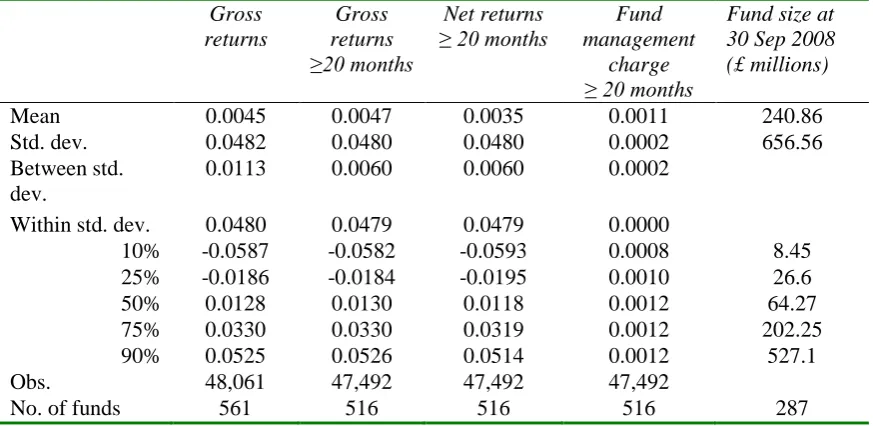
Table 3.1 provides some descriptive statistics on the returns to and the size of the mutual
funds in our dataset. The average monthly gross return across all funds (equally weighted)
and months in the data set is 0.45% (45 basis points), compared with an average monthly
return over the same sample period of 0.36% for the FT-All Share Index (not reported).17 The overall standard deviation of these returns is 4.82%, and the reported percentiles of the
distribution of returns also emphasise that there is some variability in these returns. In the
subsequent regression analysis, we require a minimum number of observations to undertake a
14 These data providers required a confidentiality clause which prohibits us from publishing their data. The
names of the 516 funds used in the main analysis of our study and the dates over which the monthly returns were available are contained in a spreadsheet on the Pensions Institute website (pensions-institute.org).
15 We analyse all the funds together in this study; we do not report the separate analysis for each sector due to
space constraints.
16 Operating costs include administration, record-keeping, research, custody, accounting, auditing, valuation,
legal costs, regulatory costs, distribution, marketing and advertising. Trading costs include commissions, spreads and taxes.
meaningful statistical analysis and we impose the requirement that time series fund
parameters are only estimated when there were 20 or more monthly gross returns reported for
that mutual fund. We also report key percentiles of the distribution of gross returns for the
sub-sample of 516 mutual funds with a minimum of 20 time-series observations, and this can
be compared with the distribution of returns across the whole sample to confirm that the
sub-sample is indeed representative.18 Overall, these results indicate that survivorship bias is negligible in this dataset. The mean monthly net return is 0.35%, implying that the mean
monthly fund management fee is 0.11%. The mean return is now very close to the mean
return of 0.36% for the FT-All Share Index. This provides initial confirmation that the
average mutual fund manager cannot “beat the market” (i.e., cannot beat a buy-and-hold
strategy invested in the market index), once all costs and fees have been taken into account.
The final column shows that the distribution of scheme size is skewed: with the median fund
value in September 2008 being £64 million and the mean value £240 million. It can be seen
that 10% of the funds have values above £527 million.
4. Results
We now turn to assessing the performance of UK equity mutual funds over the period
1998-2008. The results are divided into three sections. The first section looks at the performance of
equal- and value-weighted portfolios of all funds in the sample against the standard
four-factor benchmark model. The second section assesses the performance of the funds against
the standard and augmented benchmark models applying panel estimation methods. The third
section accounts for the non-normality of the errors in the benchmark models and undertakes
inference using panel bootstrap simulations.
4.1 Performance assessed by factor benchmark models: pooled single equation estimates
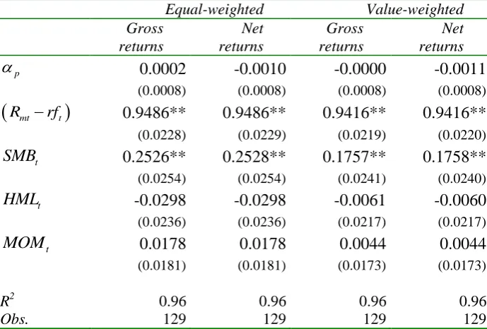
Following Blake and Timmermann (1998) and Fama and French (2010), Table 4.1 reports the
results from estimating the standard benchmark model (2.1) across all T = 129 time-series
observations, where the dependent variable is, first, the excess return on an equal-weighted
portfolio p of all funds in existence at time t, and, second, the excess return on a
value-weighted portfolio p of all funds in existence at time t, using starting market values as
18 Panel A confirms that the distribution of net returns with 20 or more observations is very similar to the
weights.19For each portfolio, the first two columns report the estimated loadings on each of the factors when the dependent variable is based on gross returns, while the second two
columns report the corresponding results using net returns. The loadings on the market
portfolio and on the SMBtfactor are positive and significant, while on the HMLt factor, the
loadings are negative but insignificant. The loadings are positive but insignificant on the
t
MOM factor.20 The insignificance of the loading on the HMLt factor – which measures the
difference in performance between growth and value stocks – indicates that there has been no
outperformance by either growth or value managers over the period. Similarly, fund
managers have not benefitted from momentum effects over the sample period.
In all cases in Table 4.1, the measure of fund manager performance alpha (p) is not
significant in the four-factor model. This result holds whether the portfolio is equal-weighted
or value-weighted, or whether we use gross returns or net returns. The implication of these
results is that the average equity mutual fund manager in the UK is unable to deliver
outperformance (i.e., unable to add value from the key active investment strategy of stock
selection), once allowance is made for fund manager charges and for a set of common risk
factors that are known to influence returns, thereby reinforcing our findings from our
examination of raw returns in Table 3.1. This is a common finding when using the standard
benchmark model (2.1), and is comparable with both previous UK (Blake and Timmermann,
1998) and the US results (Fama and French, 2010).
4.2 Performance assessed by factor and augmented benchmark models: panel regression
estimates
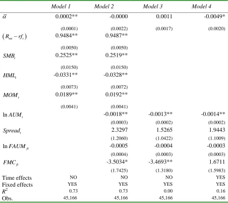
We now re-estimate these models using fixed-effects panel regressions with clustered
standard errors at the fund level. The results of these panel estimations are presented in Panel
A of Table 4.2 for gross returns and in Panel B for net returns.
19 We use the monthly FTSE All-Share Index as the market benchmark for all UK equities. We take the excess
return of this index over the UK Treasury bill rate. SMB HMLt, t, and MOMt are UK versions of the other common risk factors as defined in Gregory, Tharyan and Christidis (2013).
20 Note that the estimated factor loadings for the models where the dependent variable is based on gross returns
Model 1 is the standard four-factor benchmark model (2.1), except that the model is estimated
as a panel, so we drop the i subscript from (2.1). The results are given in the first column of
Panels A and B. We can see that for gross returns the average alpha is a significant 0.0002,
while for net returns the average alpha is a highly significant but negative –0.0010. Model 2
is the augmented specification (2.2) which includes the fund characteristics as in CHHK but
now estimated as a panel. The second column of Panels A and B shows that the coefficient on
fund size is negative and highly significant, indicating that increasing fund size has a material
effect in lowering a fund’s performance. Once we control for fund size and the other
fund-specific factors – in particular, family fund size – the average fund manager’s alpha for both
gross and net returns is insignificantly different from zero. This implies that if better qualified
managers do manage the largest funds in the largest fund families – which is entirely
plausible – they do not appear to deliver outperformance: in other words, the size of the fund
overwhelms any superior skills they might have, as predicted by Berk and Green (2004).
Model 3 is the second stage of the CHHK modelling approach, but estimated as a panel. In
the first stage, we estimate a time series model for each fund to obtain estimates of the
loadings on the four factors, and we compute the abnormal returns from this estimated
four-factor model for each fund in each month (see (2.3) above). In the second stage, we estimate
these abnormal returns on the fund-specific characteristics in a panel using fixed effects with
clustered standard errors (see (2.4) above). As with Model 2, in the third column of Panels A
and B, we can see that the coefficient on fund size is again negative and significant.
Similarly, alpha is insignificant.
Model 4 is Model 3 with time dummies. The effect of including time dummies is to render the
average fund manager’s alpha significantly negative for both gross and net returns. The
intuition for this is that there are common shocks across all mutual funds in particular
months, which are not captured by the standard common factors or the additional
fund-specific variables, but which, on average, enhance the fund’s performance. These common
shocks are unrelated to individual fund manager selectivity skills, but are being picked up in
the alpha estimates in Models 1-3, and are being wrongly attributed to manager skill.21 We needed the time dummies to separate these different effects.
21 The inclusion of the time dummies has the effect of making the coefficient on the average management
4.3 Performance assessed by simulations: non-parametric and parametric bootstraps
The panel estimation framework in Model 4, although dealing with the cross correlations in
the error terms and time effects, does not account for any non-normalities in excess returns.
We now allow for these non-normalities using non-parametric and parametric panel bootstrap
simulations.
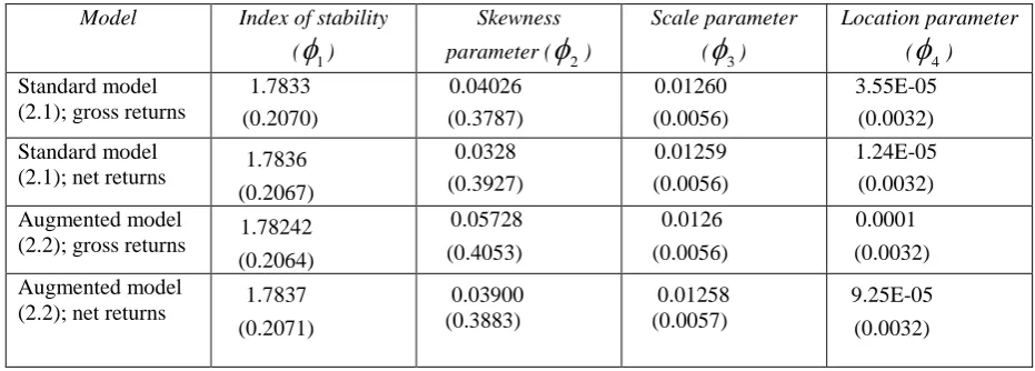
We first summarise the properties of the stable distributions underlying the panel bootstraps.
Table 4.3 presents some descriptive statistics of the estimated parameters of the stable
distributions of the residuals, ˆit, from the both the standard model (2.1) and the augmented
model (2.2). For
1
2
and
2
0
, the stable distribution reduces to the normaldistribution. As the index of stability,
1, decreases, the distribution becomes progressivelymore leptokurtic, since the tails contain increasing proportions of the probability mass. For
1
1
, the scale and location parameters,
3 and
4, can be viewed as the generalised formsof the standard deviation and the mean of the distribution, respectively.22
There is strong evidence of deviations from normality in Table 4.3 as the majority of the
estimated stability index parameters (
1) is below 2, indicating the prevalence of leptokurticdistributions.23 This departure from normality informs our parametric bootstrap, since we draw samples from the estimated stable distributions which by and large exhibit “fat tails”.
Although the moments of stable distributions such as skewness and kurtosis are not always
defined (depending upon the value of the index of stability), our bootstrap methodology takes
fully into account the existence of fat tails and skewness.
We report the bootstrap results for the augmented model (2.2). Panel A of Table 4.4
summarises the distribution of the t-statistics of the alphas based on gross returns. The first
column reports selected percentiles from the CDF of the actual t-statistics,
ˆ
{ ( ),t i i1,. . . ,516}, ranked from lowest to highest. The next two columns report the CDFs
significantly negative. The reason for this is not clear. The size and significance of the other parameters are robust to the inclusion of the time dummies.
22 It is worth mentioning here that the sum of stable distributions with the same index of stability follows a
stable distribution. Stable distribution sharing the same stability index can be first-order stochastically ordered according to their scale parameter (Rachev and Mittnik, 2000).
23
of the “luck” distributions, { (t ib),i1,. . . ,516;b1,...,10, 000} , generated by the
non-parametric and non-parametric bootstrap simulations, respectively, and again ranked from lowest
to highest. Panel B of Table 4.3 reports the same information for net returns. Figures 4.1 and
4.2 show the information in Panel B graphically. In both figures, the CDF of the actual t
-statistics lies entirely to the left of those generated by the luck distributions, implying that all
the fund managers perform worse than pure chance, once we control for the common risk
factors and key fund-specific variables, especially fund size.24 The two figures also show the 5-95% confidence intervals for the two bootstraps. In both figures, only around 1% of fund
managers generate statistically significant positive alphas, although we cannot rule out the
possibility that these alphas are generated by pure luck.
5. Conclusions
Our paper introduces two new methodologies for improving inference in the evaluation of
mutual fund performance. The first recognises the panel nature of the dataset and the
possibility that there are both fund and time effects in mutual fund returns. To account for
these, we estimate a panel regression with standard errors clustered by fund and with time
dummies to allow for time effects. The second recognises the distributional properties of the
individual mutual fund returns and the possibility that these might not be normal: a number of
recent studies have dealt with this issue using a parametric bootstrap. However, the
non-parametric bootstrap draws the observations of interest from a uniform distribution. This
method of sampling gives excessive weight by assigning equal probability of appearance to
observations that may lie in the tail of the true but unknown distribution. This can lead to
biased estimates of the confidence intervals with a coverage rate below the nominal level. To
correct for this, we use a parametric bootstrap for each fund generated by a stable distribution
calibrated to reflect the actual distribution of that fund’s returns over the sample period.
On the basis of a dataset of equity mutual funds in the UK over the period 1998-2008, we
draw the following conclusions. The standard four-factor benchmark model, estimated as a
panel regression with standard errors clustered by fund, suggests that the average UK equity
mutual fund manager does not add value relative to the benchmark once the fund
management charges are taken into account. However, the standard model excludes
fund-specific characteristics which might influence performance and ignores potential time effects
in returns. In addition, most studies using the standard model fail to take adequate account of
the non-normal distribution of the fund manager’s returns.
If we include fund size as an additional variable, then the average fund manager’s alpha over
the whole of sample period is, depending on the model, zero or significantly negative for both
gross and net returns. This confirms the earlier finding of Chen et al. (2004) and suggests that
a larger fund size helps to reduce fund performance. Since the most likely explanation for the
negative relationship between fund size and performance is the negative market impact effect
from large funds attempting to trade in size (Keim and Madhavan, 1995), this suggests that
funds should split themselves up when they get to a certain size in order to improve the return
to investors.25
The inclusion of time effects in the benchmark models further reinforces the statistical
insignificance of the average fund manager’s alpha. Our explanation for this is that there are
time effects which are not captured by the standard common factors and which, in aggregate,
enhance the average fund’s performance. But these time effects are unrelated to individual
fund manager selectivity skills, yet will have the effect of increasing the estimates of the
average fund manager’s alpha unless explicit allowance is made for them using time
dummies.
The augmented model produces even stronger evidence of the absence of fund manager skills
than the four-factor model because it conditions on a larger number of variables, so the hurdle
is higher and what is left unexplained – namely, the noise, the uncertainty, the residual
randomness – is reduced. Contained within the residual randomness of the benchmark model
is the skill of the fund manager which we capture via our estimate of alpha. The combination
of a higher hurdle and reduced noise means that fewer managers will be able to outperform.
Finally, if we allow for the normality of fund returns using a series of (both
non-parametric and non-parametric) bootstrap simulations, we find that for the augmented model,
there is no evidence that even the best performing fund managers can beat this benchmark
when allowance is made for the costs of fund management.
25 Blake, Rossi, Timmermann, Tonks and Wermers (2013) made a similar recommendation in the context of the
Table 3.1: Descriptive statistics for UK equity mutual funds 1998-2008
Gross returns
Gross returns ≥20 months
Net returns
≥ 20 months management Fund charge ≥ 20 months
Fund size at 30 Sep 2008 (£ millions)
Mean 0.0045 0.0047 0.0035 0.0011 240.86
Std. dev. 0.0482 0.0480 0.0480 0.0002 656.56
Between std. dev.
0.0113 0.0060 0.0060 0.0002
Within std. dev. 0.0480 0.0479 0.0479 0.0000
10% -0.0587 -0.0582 -0.0593 0.0008 8.45
25% -0.0186 -0.0184 -0.0195 0.0010 26.6
50% 0.0128 0.0130 0.0118 0.0012 64.27
75% 0.0330 0.0330 0.0319 0.0012 202.25
90% 0.0525 0.0526 0.0514 0.0012 527.1
Obs. 48,061 47,492 47,492 47,492
No. of funds 561 516 516 516 287
Table 4.1: Estimates of the standard benchmark model for an equal-weighted and a value-weighted portfolio of UK equity mutual funds 1998-2008
Equal-weighted Value-weighted
Gross returns
Net returns
Gross returns
Net returns
p
0.0002 -0.0010 -0.0000 -0.0011
(0.0008) (0.0008) (0.0008) (0.0008)
Rmt rft
0.9486** 0.9486** 0.9416** 0.9416**(0.0228) (0.0229) (0.0219) (0.0220)
t
SMB 0.2526** 0.2528** 0.1757** 0.1758**
(0.0254) (0.0254) (0.0241) (0.0240)
t
HML -0.0298 -0.0298 -0.0061 -0.0060
(0.0236) (0.0236) (0.0217) (0.0217)
t
MOM 0.0178 0.0178 0.0044 0.0044
(0.0181) (0.0181) (0.0173) (0.0173)
R2 0.96 0.96 0.96 0.96
Obs. 129 129 129 129
Table 4.2: Panel estimates of the standard and augmented benchmark models of UK equity mutual funds 1998-2008
Panel A: Gross returns
Model 1 Model 2 Model 3 Model 4
0.0002** -0.0000 0.0011 -0.0049*
(0.0001) (0.0022) (0.0017) (0.0020)
Rmt rft
0.9484** 0.9487**(0.0050) (0.0050)
t
SMB 0.2525** 0.2519**
(0.0150) (0.0150)
t
HML -0.0331** -0.0328**
(0.0073) (0.0072)
t
MOM 0.0189** 0.0192**
(0.0041) (0.0041)
lnAUM t -0.0018** -0.0013** -0.0014**
(0.0003) (0.0002) (0.0002)
t
Spread 2.3297 1.5265 1.9443
(1.2060) (1.0422) (1.1009)
lnFAUMft -0.0005 -0.0004 -0.0003
(0.0004) (0.0003) (0.0003)
ft
FMC -3.5034* -3.4693** 1.6711
(1.7425) (1.3180) (1.5983)
Time effects NO NO NO YES
Fixed effects YES YES YES YES
R2 0.73 0.73 0.00 0.16
Panel B: Net returns
Model 1 Model 2 Model 3 Model 4
-0.0010** -0.0003 0.0008 -0.0053**
(0.0001) (0.0022) (0.0017) (0.0020)
Rmt rft
0.9484** 0.9487**(0.0050) (0.0050)
t
SMB 0.2525** 0.2519**
(0.0150) (0.0150)
t
HML -0.0331** -0.0328**
(0.0073) (0.0072)
t
MOM 0.0189** 0.0192**
(0.0041) (0.0041)
lnAUM t -0.0018** -0.0013** -0.0014**
(0.0003) (0.0002) (0.0002)
t
Spread 2.2560 1.4561 1.8747
(1.2113) (1.0452) (1.1042)
lnFAUMft -0.0005 -0.0004 -0.0003
(0.0004) (0.0003) (0.0003)
ft
FMC -4.1689* -4.1141** 1.0778
(1.7551) (1.3338) (1.6083)
Time effects NO NO NO YES
Fixed effects YES YES YES YES
R2 0.73 0.73 0.00 0.16
Obs. 45,166 45,166 45,166 45,166
In Panel A, Model 1 is the standard four-factor benchmark model (2.1) for excess gross returns as the dependent variable. Model 2 is the augmented benchmark model (2.2) for excess gross returns, including fund-specific variables, but without any time effects. Model 3 follows Chen et al. (2004) and involves a two-stage estimation procedure: in stage 1, equation (2.1) is estimated for each fund separately, and abnormal gross returns are defined by equation (2.3); in stage 2, the estimated model is equation (2.4) but without time effects. Model 4 is Model 3 with bi-monthly time effects. In Panel B, the estimated models are the same as in Panel A, but with excess net returns as the dependent variable. The dependent variables in these panel regressions are based on the monthly returns on the 516 mutual funds that were in the dataset for at least 20 months for some time between January 1998 and September 2008 (129 months). The estimates of the parameters , , , in the standard model and , , , , , , , in the augmented model are the same for all funds. Estimates of the additional fund-specific “skill” levels, i,
and the time effects , t, are not reported. The standard errors are clustered in the fund dimension: ***, **
Table 4.3: Means and standard deviations of the parameters of the stable distributions fitted to the estimated residuals of the standard and augmented benchmark models
Model Index of stability
(
1)Skewness
parameter (
2)Scale parameter
(
3)Location parameter
(
4)Standard model (2.1); gross returns
1.7833 (0.2070) 0.04026 (0.3787) 0.01260 (0.0056) 3.55E-05 (0.0032) Standard model
(2.1); net returns 1.7836
(0.2067) 0.0328 (0.3927) 0.01259 (0.0056) 1.24E-05 (0.0032) Augmented model
(2.2); gross returns 1.78242 (0.2064) 0.05728 (0.4053) 0.0126 (0.0056) 0.0001 (0.0032) Augmented model
(2.2); net returns 1.7837
(0.2071) 0.03900 (0.3883) 0.01258 (0.0057) 9.25E-05 (0.0032)
The residuals from four benchmark models – the standard model (2.1) where the dependent variable is excess gross returns, the standard model (2.1) where the dependent variable is excess net returns, the augmented model (2.2) where the dependent variable is excess gross returns, and the augmented model (2.2) where the dependent variable is excess net returns – for each of the 516 mutual funds that were in the dataset for at least 20 months for some time between January 1998 and September 2008 (129 months) were fitted to a stable distribution. For
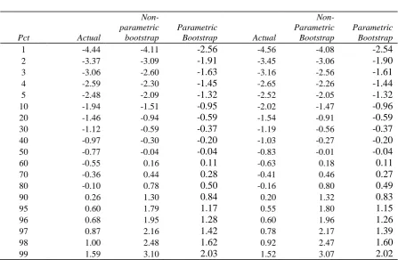
Table 4.4: Percentiles of the actual and average non-parametric and parametric bootstrap cumulative distribution functions of the t-statistics on alpha in the augmented benchmark model for the gross and net returns on UK equity mutual funds 1998-2008
Panel A: Gross Returns Panel B: Net Returns
Pct Actual
Non-parametric
bootstrap
Parametric
Bootstrap Actual
Non-Parametric
Bootstrap
Parametric Bootstrap
1 -4.44 -4.11 -2.56 -4.56 -4.08 -2.54
2 -3.37 -3.09 -1.91 -3.45 -3.06 -1.90
3 -3.06 -2.60 -1.63 -3.16 -2.56 -1.61
4 -2.59 -2.30 -1.45 -2.65 -2.26 -1.44
5 -2.48 -2.09 -1.32 -2.52 -2.05 -1.32
10 -1.94 -1.51 -0.95 -2.02 -1.47 -0.96
20 -1.46 -0.94 -0.59 -1.54 -0.91 -0.59
30 -1.12 -0.59 -0.37 -1.19 -0.56 -0.37
40 -0.97 -0.30 -0.20 -1.03 -0.27 -0.20
50 -0.77 -0.04 -0.04 -0.83 -0.01 -0.04
60 -0.55 0.16 0.11 -0.63 0.18 0.11
70 -0.36 0.44 0.28 -0.41 0.46 0.27
80 -0.10 0.78 0.50 -0.16 0.80 0.49
90 0.26 1.30 0.84 0.20 1.32 0.83
95 0.60 1.79 1.17 0.55 1.80 1.15
96 0.68 1.95 1.28 0.60 1.96 1.26
97 0.87 2.16 1.42 0.78 2.17 1.39
98 1.00 2.48 1.62 0.92 2.47 1.60
99 1.59 3.10 2.03 1.52 3.07 2.02
The results are based on the augmented benchmark model (2.2), including fund-specific variables and time effects, where the dependent variable is based on the monthly returns on the 516 mutual funds that were in the dataset for at least 20 months for some time between January 1998 and September 2008 (129 months). Panel A reports the results for excess gross returns, while Panel B reports the results for excess net returns. Each panel shows, for selected percentiles (Pct) of the cumulative distribution function, the value of the
actual t-statistic of the estimated alpha, { ( ),t ˆi i1,. . . ,516}, after the 516 t-statistics have been ranked from smallest to largest (Actual). It also shows, for the same percentiles of the cumulative distribution
[image:24.595.71.519.137.429.2]
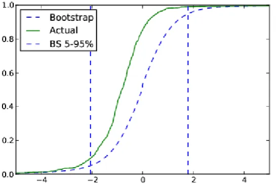
Figure 4.1: The actual and average non-parametric bootstrap cumulative distribution functions of the t-statistics on alpha in the augmented benchmark model for the net returns on UK equity mutual funds 1998-2008
The results are based on the augmented benchmark model (2.2), including fund-specific variables and time effects, where the dependent variable is the monthly excess net returns on the 516 mutual funds that were in the dataset for at least 20 months for some time between January 1998 and September 2008 (129 months). The solid curve (labelled “Actual”) is the cumulative distribution function of the values of the actual t
-statistics of the estimated alphas, { (t ˆi),i1,. . . ,516}, after the 516 t-statistics have been ranked from smallest to largest. The dashed curve (labelled “Bootstrap”) is the cumulative distribution function of the
[image:25.595.97.370.140.330.2]
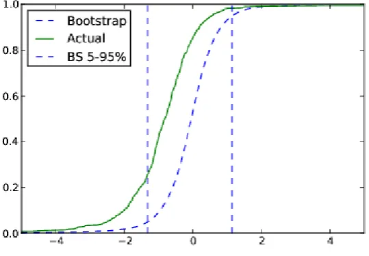
Figure 4.2: The actual and average parametric bootstrap cumulative distribution functions of the t-statistics on alpha in the augmented benchmark model for the net returns on UK equity mutual funds 1998-2008
The results are based on the augmented benchmark model (2.2), including fund-specific variables and time effects, where the dependent variable is the monthly excess net returns on the 516 mutual funds that were in the dataset for at least 20 months for some time between January 1998 and September 2008 (129 months). The solid curve (labelled “Actual”) is the cumulative distribution function of the values of the actual t -statistics of the estimated alphas, { ( ),t ˆi i1,. . . ,516}, after the 516 t-statistics have been ranked from
smallest to largest. The dashed curve (labelled “Bootstrap”) is the cumulative distribution function of the
[image:26.595.97.367.132.319.2]
References
Barras, L., O. Scaillet and R. Wermers (2010). "False discoveries in mutual fund performance: Measuring luck in estimated alphas." Journal of Finance 65(1): 179-216.
Beran, R. (1987). "Prepivoting to reduce level error of confidence sets." Biometrika 74(3): 457-468.
Beran, R. (1990). "Refining bootstrap simultaneous confidence sets." Journal of the American Statistical Association 85(410): 417-426.
Berk, J. B. and R. C. Green (2004). "Mutual fund flows and performance in rational markets." Journal of Political Economy 112(6): 1269-1295.
Bhargava, A. (1987). "Wald tests and systems of stochastic equations." International Economic Review 28(3): 789-808.
Bhargava, A., L. Franzini and W. Narendranathan (1982). "Serial correlation and the fixed effects model." The Review of Economic Studies 49(4): 533-549.
Blake, D., A. Rossi, A. Timmermann, I. Tonks, and R. Wermers (2013). "Decentralized investment management: Evidence from the pension fund industry." Journal of Finance 68(3): 1133–1178.
Blake, D. and A. Timmermann (1998). "Mutual fund performance: Evidence from the UK." European Finance Review 2(1): 57-77.
Carhart, M. (1997). "On persistence in mutual fund performance." Journal of Finance 52(1): 57-82.
Carpenter, J. N., and A. W. Lynch (1999). "Survivorship bias and attrition effects in measures of performance persistence." Journal of financial economics 54(3): 337-374.
Chambers, J. M., C. L. Mallows and B. Stuck (1976). "A method for simulating stable random variables." Journal of the American Statistical Association 71(354): 340-344.
Chen, J., H. Hong, M. Huang and J. D. Kubik (2004). "Does fund size erode mutual fund performance? The role of liquidity and organization." American Economic Review 94(5): 1276-1302.
Chen, J., H. Hong, W. Jiang and J. D. Kubik (2013). "Outsourcing mutual fund management: Firm boundaries, incentives, and performance." Journal of Finance 68(2): 523-558.
Chevalier, J. and G. Ellison (1999a). "Are some mutual fund managers better than others? Cross‐ sectional patterns in behavior and performance." Journal of Finance 54(3): 875-899.
Chevalier, J. and G. Ellison (1999b). "Career concerns of mutual fund managers." Quarterly Journal of Economics 114(2): 389-432.
Cohen, L., A. Frazzini and C. Malloy (2008). "The small world of investing: Board connections and mutual fund returns." Journal of Political Economy 116(5): 951-979.
Elton, E. J., M. J. Gruber and C. R. Blake (1996). "Survivor bias and mutual fund performance." Review of Financial Studies 9(4): 1097-1120.
Fama, E.F., and K. R. French (1993). "Common risk factors in the returns on stocks and bonds." Journal of Financial Economics 33, 3–56.
Fama, E. F. and K. R. French (2010). "Luck versus skill in the cross-section of mutual fund returns." Journal of Finance 65(5): 1915-1947.
Fama, E. F. and J. D. MacBeth (1973). "Risk, return, and equilibrium: Empirical tests." Journal of Political Economy 81(3): 607-636.
Ferson, W.E., and R. W. Schadt (1996). "Measuring fund strategy and performance in
changing economic conditions." Journal of Finance51, 425–461.
Gregory, A., R. Tharyan and A. Christidis (2013). "Constructing and testing alternative versions of the Fama–French and Carhart models in the UK." Journal of Business Finance & Accounting 40(1-2): 172-214.
Hahn, J. and G. Kuersteiner (2002). "Asymptotically unbiased inference for a dynamic panel model with fixed effects when both n and T are large." Econometrica 70(4): 1639-1657.
Henriksson, R. D. and R. C. Merton (1981). "On market timing and investment performance. II. Statistical procedures for evaluating forecasting skills." Journal of business 54(4): 513-533.
Hong, H., J. D. Kubik and J. C. Stein (2005). "Thy neighbor's portfolio: Word-of-mouth effects in the holdings and trades of money managers." Journal of Finance 60(6): 2801-2824.
Hsiao, C. (1986). Analysis of Panel Data. Cambridge: Cambridge University Press.
IMSL (1985). User's Manual. Houston, TX: IMSL Library.
Jensen, M. C. (1968). "The performance of mutual funds in the period 1945-1964." Journal of Finance 23(2): 389-416.
Kapetanios, G. (2008). "A bootstrap procedure for panel data sets with many cross‐sectional units." The Econometrics Journal 11(2): 377-395.
Keim, D. B. and A. Madhavan (1995). "Anatomy of the trading process empirical evidence on the behavior of institutional traders." Journal of Financial Economics 37(3): 371-398.
Khorana, A. (1996). "Top management turnover: An empirical investigation of mutual fund managers." Journal of Financial Economics 40(3): 403-427.
Kosowski, R., A. Timmermann, R. Wermers and H. White (2006). "Can mutual fund 'stars' really pick stocks? New evidence from a bootstrap analysis." Journal of Finance 61(6): 2551-2595.
Martin, M. A. (1990). "On bootstrap iteration for coverage correction in confidence intervals." Journal of the American Statistical Association 85(412): 1105-1118.
Massa, M. (2003). "How do family strategies affect fund performance? When performance-maximization is not the only game in town." Journal of Financial Economics 67(2): 249-304.
Nanda, V., Z. J. Wang and L. Zheng (2004). "Family values and the star phenomenon: Strategies of mutual fund families." Review of Financial Studies 17(3): 667-698.
Neyman, J. and E. L. Scott (1948). "Consistent estimates based on partially consistent observations." Econometrica 16(1): 1-32.
Nickell, S.J. (1981). "Biases in dynamic models with fixed effects." Econometrica 49(6): 1417-1426.
Nolan, J. P. (1997). "Numerical calculation of stable densities and distribution functions." Communications in statistics - Stochastic models 13(4): 759-774.
Petersen, M. A. (2009). "Estimating standard errors in finance panel data sets: Comparing approaches." Review of Financial Studies 22(1): 435-480.
Rachev, S. T., and S. Mittnik (2000) Stable Paretian Models in Finance. Chichester & New York: Wiley.
Sirri, E. R. and P. Tufano (1998). "Costly search and mutual fund flows." Journal of Finance 53(5): 1589-1622.
Treynor, J. and K. Mazuy (1966). "Can mutual funds outguess the market." Harvard Business Review 44(4): 131-136.
White, H. (1980). "A heteroskedasticity-consistent covariance matrix estimator and a direct test for heteroskedasticity." Econometrica 48(4): 817–838.
Yan, X. S. (2008). "Liquidity, investment style, and the relation between fund size and fund performance." Journal of Financial and Quantitative Analysis 43(3): 741-767.