CHARMM force field parameterization protocol for self-assembling peptide amphiphiles : the Fmoc moiety

Journal Name

ARTICLE

Received 00th January 20xx, Accepted 00th January 20xx

DOI: 10.1039/x0xx00000x

www.rsc.org/

CHARMM force field parameterization protocol for

self-assembling peptide amphiphiles: The Fmoc moiety

I. Ramos Sasselli,a R. V. Ulijna,b and T. Tuttlea,*

Aromatic peptide amphiphiles are known to self-assemble into nanostructures but the molecular level structure and the mechanism of formation of these nanostructures is not yet understood in detail. Molecular Dynamic simulations using the CHARMM force field have been applied to a wide variety of peptide-based systems to obtain molecular level details of processes that are inaccessible with experimental techniques. However, this force field does not include parameters for the aromatic moieties which dictate the self-assembly of these systems. The standard CHARMM force field parameterization protocol uses hydrophilic interactions for the non-bonding parameters evaluation. However, to effectively reproduce the self-assembling behaviour of these molecules, the balance between the hydrophillic and hydrophobic nature of the molecule is essential. In this work, a modified parameterization protocol for the CHARMM force field for these aromatic moieties is presented. This protocol is applied for the specific case of the Fmoc moiety. The resulting set of parameters satisfies the conformational and interactions analysis and is able to reproduce experimental results such as the Fmoc-S-OMe water/octanol partition free energy and the self-assembly of Fmoc-S-OH and Fmoc-Y-OH into spherical micelles and fibres, respectively, while also providing detailed information on the mechanism of these processes. The effectiveness of the parameters for the Fmoc moiety validates the protocol as a robust approach to paramterise this class of compounds.

Introduction

Peptides are known to self-assemble into nanostructures with very interesting applications in nanotechnology and biomedicine.1-3 The supramolecular functionality of peptide-based nanomaterials is due not only to the functional groups present in the molecules but also due to the supramolecular structures formed.4 Self-assembly is a spontaneous process driven by intermolecular interactions such as electrostatic interactions, hydrogen bonding, π-stacking and the hydrophobic effect. The amino acid sequence of the peptide building blocks affects the ability of the peptide to form these interactions and, therefore, different amino acids sequences can lead to different structure types such as fibres, ribbons, tubes, and sheets.5-8 Understanding how the amino acid sequence affects the final structure is of particular interest for elucidating the “design rules” for peptide based nanomaterials.

Computational methods have been employed with

significant success to reveal both molecular level detail and the mechanism of formation for a range of peptide-based nanostructures. Molecular Dynamics (MD) simulations have been applied to increase the understanding of different features of peptide-based nanomaterials at the molecular level.9, 10 In particular, coarse grain (CG) simulations have been increasingly utilized to illustrate the aggregation of peptides and peptide amphiphiles (PA).11 CG simulations have also provided insights into different self-assembling mechanism by studying the free energy profiles of these processes,12 and a systematic CG screening approach was applied to all possible di- and tripeptides and has successfully described literature examples of assembled peptides and predicted the self-assembling tendency of other peptides that could subsequently be verified by experimentation.13, 14

Atomistic MD simulations have also been used in the area of self-assembling materials, although primarily this has been to study the preferred conformations of the peptides or PA in the assembled state.15-17 Atomistic simulations are limited to smaller sizes than CG and require substantially more computation time but they have the advantage of atomistic resolution, which is required for the study of the specific non-covalent interactions involved in the self-assembly process. Free energy profile studies using atomistic MD simulations have also been successfully applied for the study of self-assembling mechanism of aliphatic PAs.18, 19

N-terminus with an aromatic group.20-22 The formation of extra π-stacking interactions by the aromatic group facilitates the self-assembly in these systems and allows shorter peptides to form nanostructures.23 Several di- and tripeptides bound to the fluorenyl-9-methoxycarbonyl (Fmoc) group have been found to form nanostructures which are strongly dependent of the amino acid sequence (e.g., Fmoc-TF-OMe self-assembles into fibres while Fmoc-SF-OMe forms sheets).4, 5, 7, 24-26 There are even examples of single amino acids protected with the Fmoc moiety which are able to form nanostructures.27-29 As such, this class of compounds represent a highly tuneable set of PAs that may be used for a wide range of applications. Remarkably, it is not only the fluorenyl group but also the specific geometry of the methoxycarbonyl linker which aids in the self-assembly process as was recently demonstrated by varying the linker between fluorenyl and peptide for Fmoc-YL.30

As in the case of other PAs, the structures formed by Fmoc-peptides are not fully understood and often discovered by chance rather than rational molecular design. MD methods have been already applied to these systems in order to gain understanding on the preferred conformations of these molecules in the self-assembled state and on the importance of the different interactions in the self-assembling mechanism.15, 31-33 However, the implementation of simulations for these systems has an added difficulty which is that the force fields used for the simulations do not include parameters for the Fmoc moiety. Therefore, the first step for the use of MD methods in Fmoc-peptides self-assembly is the parameterization of this aromatic moiety. As the quality of the results obtained in subsequent simulations – particularly in the case of unbiased, long timescale simulations – will be dependent on the quality of the parameters used, an accurate and consistent parameterization of the Fmoc moiety is critical.

Force field parameters are typically obtained either from experimental results or quantum mechanical data (QM).34-37 The molecules used to derive these parameters and the way they are obtained and optimized are characteristic of a force field and limit its applications. The CHARMM force field was chosen to simulate the self-assembling peptide based systems as it is parameterized and well validated for proteins and peptides.34, 38 The CHARMM force field includes parameters for many organic molecules (including fluorene and other aromatic groups), lipids, nucleic acids, and some carbohydrates.38-40 It is common when parameterizing a new molecule in a force field which includes parameters for such a wide range of molecules to obtain the bonded parameters from similar segments of molecules already parameterized for that force field.31, 41, 42 However, the non-bonded parameters, electrostatic and van der Waals, need to be optimized. As these parameters may have an influence in the torsional potentials, the torsional parameters also need to be optimized. The CHARMM parameterization protocol evaluates the interactions of the hydrophilic parts of a given molecule with water.34, 39, 40 Nevertheless, to reproduce the self-assembling behaviour of aromatic peptide amphiphiles a balance between

essential. Therefore, in this study we present a modified protocol to parameterize aromatic moieties, within the CHARMM force field, that are used to form aromatic peptide amphiphiles. The protocol is presented for the Fmoc moiety due to the high prevalence of Fmoc-peptide amphiphiles as self-assembling molecules.29

This study is presented starting with the parameterization of the Fmoc moiety, which includes: the derivation of the bonded parameters from parameterized molecules with similar segments; the charges and van der Waals terms optimization; and the torsional terms optimization. The second part of the study is focused in the validation of the parameterization: firstly comparing the partition coefficient of Fmoc-S-OMe obtained computationally with the partition coefficient measured experimentally; and secondly by using the parameters to study self-assembling systems whose final structures are well known.

Parameterization of Fmoc

The parameterization was made for the CHARMM force field, which includes parameters for amino acids as well as a wide range of other organic molecules. To parameterize the Fmoc moiety some of the parameters where extrapolated from similar molecules or molecules which present the same chemical groups of the CHARMM parameters library.

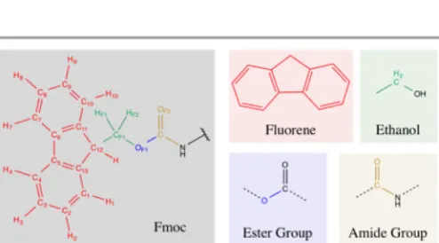
The parameters for 9-fluorenylmethyloxycarbonyl or the Fmoc moiety were obtained as follows. For the fluorenyl group the parameters were taken from the fluorene molecule (Figure 1, Red); for the –CH2– which links the aromatic part to the group to the oxygen, the parameters were taken from ethanol (Figure 1, Green); the parameters for the following oxygen (– O–) were obtained from standard ester groups (Figure 1, Blue) and parameters from general amides were used for the carbonyl group (C=O) (Figure 1, Orange).

The CHARMM force field presents the following expression for the energy:

𝐸!"! 𝑟 = 𝑘! 𝑟−𝑟!,! ! !"#$%

+ 𝑘!" 𝑆−𝑆!,!" ! !"

+ 𝑘! 𝜃−𝜃!,! !

!"#$%

+ 𝑘!,! 1+𝑐𝑜𝑠 𝑛𝜒−𝛿!,!

!"!!"#$%&

+ 𝑘! 𝜓−𝜓!,! !

!"#$%#&$'

+ 𝜀!"

𝑅!"#,!" 𝑟!"

!"

−2 𝑅!"#,!" 𝑟!"

!

!"#

+ 𝑞!𝑞!

4𝜋𝜀!𝑟!" !"!#$%&'$($)#

𝐸𝑞.1

This equation has seven different terms. The force constants (kb, kUB, ka, ki) and reference values (r0,b , S0,UB, θ0,a,

ψ0,i) for the bonds stretching, Urey-Bradley terms, angles bending and improper dihedrals were directly transferred from the above-mentioned groups in the CHARMM library. For the Lennard-Jones term, although other parameters (εij, Rmin,ij) were tested, they did not improve the results obtained from those transferred from the same groups of the CHARMM library, hence, the transferred parameters from the mentioned segments were also used for the Lennard-Jones term. The dihedral terms (kd,n, n, δd,n) for the fluorenyl were also taken from the fluorene molecule. Therefore the parameterization effort was focused on the dihedral terms of the linker between the aromatic group and the peptide and on the charges (qi/j), which cannot be directly transferred from the segments. QM and MM binding energies: Fmoc – Water. To calculate the binding energies of Fmoc with water the molecule Fmoc-NH2 (Figure 2) was used. This molecule was optimized at the QM level of theory. The parameterization protocol for CHARMM uses the Hartree-Fock method with the 6-31G* basis set for the binding energies calculations.39 _{However, this current work} includes the calculation of binding energies between water and the aromatic group, where dispersion forces may play an important role. As Hartree-Fock is unable to describe dispersion, the QM calculations were carried out using the DFT functional B97-D,43 _{with the basis set def2-SVP,}44 _in Turbomole.45, 46 _{The MM binding energies were calculated} using the CHARMM force field with the Fmoc parameters in the NAMD programme.47

The optimized geometry of Fmoc-NH2 was fixed for all the

Fmoc – Water QM binding energies calculation. The geometry of water was also fixed in these calculations with the TIP3P geometry.48 Therefore, the binding energies (BEs) for the Fmoc – Water systems are purely interaction energies. The different

Fmoc – Water systems were built in Avogadro.49 The QM optimized structures were used for the calculation of the MM binding energies. The Fmoc – Water binding energies (BEw) are calculated as the energy difference between each Fmoc – Water system (𝐸!"#$%⋯!"#$!!"!) and the sum of the internal energies of Fmoc-NH2 𝐸!"#$!!"! and water (𝐸!"#$%) (Equation 2).

𝐵𝐸!=𝐸!"#$%⋯!"#$!!"!− 𝐸!"#$%+𝐸!"#$!!"! (𝐸𝑞.2)

The CHARMM parameterization protocol uses the QM reference binding energies (BEQM) to optimize hydrogen bonds with water.34, 39, 40 However, in this work the binding energies of water with hydrophobic parts, not able to form hydrogen bonds, are also studied. This was done in order to include an additional reference to account for the hydrophilicity/hydrophobicity of the different parts of the moiety. The water – water binding energy (BEw-w) calculated from two water molecules with TIP3P geometry, is used as a reference point to determine the relative strength of the interactions. All BEw lower than this reference are considered hydrophilic, and those higher than the reference, hydrophobic. Therefore, the Final Charges Set (FCS) has to satisfy both conditions: the hydrophobic/hydrophilic behaviour of the different parts of the moiety (BEw-w) and the relative intensities of the interactions (BEQM).

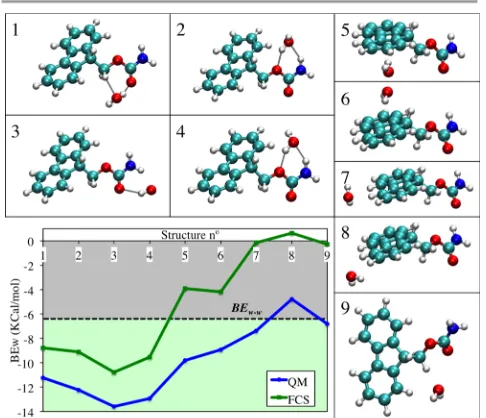
The optimized structures for the Fmoc – Water are shown in Figure 3. Structures 1 to 4 involve interactions of the water molecule with the hydrophilic parts of the Fmoc moiety, while in the structures 5 to 9 the water molecule interacts with the

Figure 2. Fmoc-NH2 model molecule in 2D (a) and 3D (b) representations.

Figure 3. Optimized geometries of the Fmoc – Water systems and BEw graph for

FCS (bottom left). The graph includes two references: the dashed black line (BEw-w) separates the hydrophobic (grey) and the hydrophilic (lime) regions; and the BEQM

hydrophobic parts of the moiety. Therefore the BEw,1-4 are expected to be lower than the BEw-w (lime area of the graph, Figure 3), while the BEw,5-9 must be higher than this reference value (grey area of the graph, Figure 3).

The FCS successfully reproduces the hydrophilic/hydrophobic behaviour of each part of the Fmoc moiety (Figure 3). Furthermore, the FCS reproduces also the shape of the BEQM and therefore the relative intensities of the interactions are in good agreement with the QM reference. The interactions 7 to 9, which involve the interaction of the water molecule with the edges of the aromatic group, are very weak or, even, repulsive. As this was found to happen for all charges sets trialled, it was assumed to be a limitation of the force field to reproduce this kind of interaction. Overall, the averaged absolute error for the Fmoc – Water binding energies is 4.6 Kcal/mol, which is within the typical error limit of force fields.

QM and MM binding energies: Fmoc – Fmoc systems. Once the FCS was obtained, it was tested against unique interactions that the Fmoc parameters should reproduce to reliably describe the self-assembling behaviour, namely, the

Fmoc – Fmoc interactions. Various configurations of two Fmoc-NH2 molecules were built in Avogadro. The systems were optimized in Turbomole using the DFT functional B97-D with the def2-SVP basis set. The optimized geometries were used to calculate the MM energy using the CHARMM force field with the Fmoc parameters in the NAMD program. The binding energies (BEdimer) are defined as the difference in energies between the system with two Fmoc molecules interacting (E!"#$!!"!⋯!"#$!!"!) and twice the internal energy of the Fmoc-NH2 molecule (E!"#$!!"!) (Equation 3). For the Fmoc –

Fmoc systems the BEdimer are not purely interactions energies but they include the internal energy change.

𝐵𝐸!"#$%=𝐸!"#$!!"!⋯!"#$!!"!− 2∙𝐸!"#$!!"! (𝐸𝑞.3)

The MM binding energies calculated using the FCS(BEFmoc) for these interactions are compared with QM calculated reference binding energies (BEQM). The final geometries and BE are presented in Figure 4. Seven different types of π-stacking interactions are studied. Six of the BE values are well reproduced as the BEFmoc calculated with the FCS are within 4.5

Kcal/mol from the BEQM. The only interaction that cannot be reproduced corresponds to the geometry p_T1 (Figure 4). This geometry involves the interactions of the aromatic group of one Fmoc-NH2 with the hydrophilic part of the other molecule. As in the case of the Fmoc – Water systems 7 to 9, this is accepted as a limitation of the force field to reproduce some types of interactions. Nonetheless, the ability to successfully reproduce the six π-stacking Fmoc – Fmoc interactions is encouraging and suggests the correct balance between the hydrophobic and hydrophilic nature of the moiety has been achieved. Furthermore, for the Fmoc – Fmoc binding energies, the averaged absolute error is 4.6 Kcal/mol, which is consistent with the error of the Fmoc – Water interactions and hence, it is also within the general accuracy of force fields.

Torsion angle parameterization. Standard amide and ester dihedral terms were used to build the dihedrals of the linker of the Fmoc. The validity of these terms was evaluated with the

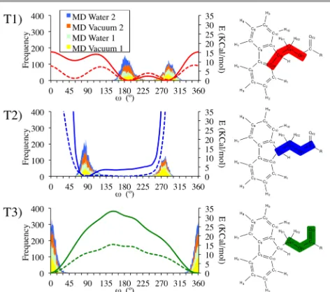
FCS and compared with reference QM values in order to accurately reproduce the flexibility of the Fmoc moiety. The dihedral angles under study were C13 – C12 – CF1 – OF1 (T1), C12 – CF1 – OF1 – C (T2) and CF1 – OF1 – C – OF2 (T3), see Figure 1 for atom names. Torsional potential profiles were calculated in Gaussian 0950 with the B3LYP51, 52 functional and the 6-31G(d,p) basis set.53, 54 The profiles were obtained with rigid scans, calculating the single point energies of structures generated via 10º of rotation around each dihedral. The MM torsional potential profiles were obtained using the same geometries and calculating the energy for the CHARMM force filed with the Fmoc parameters using the NAMD program.

As well as the static MM energies, the QM torsion potentials were compared with the distribution of the three dihedrals during 10 ns MD simulations with a single molecule of Fmoc-NH2(System 1); and with a single molecule of

Fmoc-S-Figure 4. Optimized geometries of the Fmoc – Fmoc systems and BEdimer graph for the FCS and the QM reference (top right).

OH (System 2). These simulations reveal the influence of incorporating the parameters of the Fmoc moiety to the parameters of the amino acids in CHARMM. Both systems were simulated in vacuum and in water (TIP3P model). The systems were built in VMD and were minimized with the steep descent technique to avoid high-energy contacts and equilibrated at 298 K before the simulations. The 10 ns simulations were carried out within the NVT ensemble and a 1.0 fs integration time step was applied. Results are shown in Figure 5.

The MM potentials successfully reproduce the shape of the QM references (Figure 5) although the energy barriers are typically higher relative to the QM gas phase results. The distribution of dihedrals in the simulations maps well on to the QM potentials, with the majority of the torsional space explored around the regions where the potential energy is at a minimum. It can be seen that for the dihedral T2 both, the MM and the QM barriers are much higher than for the other two dihedrals. This is caused by the proximity of the oxygen in the carbonyl group with the fluorenyl group during the rotation around T2 for the region between 270º and 45º degrees due to the use of a rigid scan, which cannot relax in each point of the rotation. This also causes a displacement for T2 in the simulations, which shows a peak between 255º and 300º that is displaced to the right in reference to the energy potentials. This shift is caused by the difference in mobility of the systems used to calculate the different parameters: the histograms are calculated from simulations where the whole molecule can move while the QM and MM plots are calculated by rotating the dihedrals in fixed molecules. Given the agreement between the QM and MM torsional profiles and the distribution of the torsional angles from the MD simulations, the flexibility in the carbamate region of the Fmoc moiety is considered to be well reproduced.

Validation via the Partition Coefficient

As an initial validation of the parameterization carried out for the Fmoc moiety, a physical parameter, which can be directly compared with the experimental observable, is calculated. Due the amphiphilic nature of the molecules for which the Fmoc moiety is parameterized, Fmoc-peptides, and the importance of reproducing this for the self-assembly simulations, the partition coefficient between octanol and water was chosen for this purpose.

Partition coefficient determination.The molecule chosen for this validation was Fmoc-S-OMe. This serine is capped at the N-terminus with the Fmoc moiety and at the C-terminus as a methyl ester. Neither of these groups nor the serine side chain contain acidic hydrogen and therefore it is not necessary to take into account any ionization effects, which simplifies the comparison of experimental and computational results. The serine side chain was chosen due to its hydrophilicity, which facilitates the experimental determination of the log P.

The experimental partition coefficient is determined by the shake flask methodology55-57 as an average of 9 samples. The details of the experiment are included in the ESI. The partition

free energy (∆Gow) is related to the partition coefficient (Kow) using Equation 4:

∆𝐺!"=2.303 𝑅𝑇 𝑙𝑜𝑔𝐾!" (𝐸𝑞.4)

The theoretical partition free energy can be calculated from the solvation free energy data of a given molecule in water (∆Gw) and in octanol (∆Goc) as shown in Equation 5:

∆𝐺!"= ∆𝐺!"−∆𝐺! (𝐸𝑞.5)

The theoretical solvation free energies in water (∆Gw) and in octanol (∆Goc) were calculated using alchemical methods, specifically free energy perturbation (FEP).58, 59

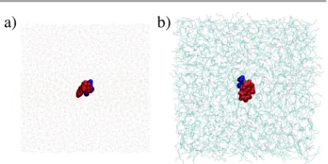
The two systems were built in VMD,60 _{both include an} Fmoc-S-OMe molecule which is surrounded by TIP3P water48 for ∆Gw (Figure 6a) and by octanol for ∆Goc (Figure 6b). The systems were built to be 60 x 60 x 60 Å of each solvent with the Fmoc-S-OMe placed in the centre of each phase. All MD calculations were carried out using the NAMD program and the CHARMM force field including the Fmoc parameterization presented in this paper. The systems were minimized to avoid bad contacts and then heated up and equilibrated at 298 K and 1 atm (NPT ensemble) for 5 ns fixing the position of Fmoc-S-OMe. A 2 fs time step and periodic boundary conditions in the three spatial coordinates61 _{were used as well as a 12 Å cut-off} for non-bonded interactions. Langevin dynamics were used for the temperature control and Langevin piston Nose-Hoover algorithm was used to keep the pressure constant.62 _The density of both systems was calculated after this equilibration step to be 0.943 g/ml for water and 0.805 g/ml for the octanol, which are reasonably similar to the experimental values of 1.000 g/ml and 0.824 g/ml, respectively.

Although water is known to be soluble in octanol (0.255 mole fraction) and hence, experimentally, some water will pass to the octanol phase, it has been demonstrated that computationally the addition of the appropriate number of water molecules into the octanol phase has a minimum effect, and the results for the dry octanol are slightly more accurate than those with the wet octanol.63

The FEP calculations were carried out using the same general MD parameters described before. Alchemical transformation was applied to decouple the Fmoc-S-OMe from the solvent. A decoupling constant dλ=0.0625 was used, giving

rise to up to 16 windows in the disappearance of Fmoc-S-OMe (from λ=0, Fmoc-S-OMe in solution, to λ=1, no Fmoc-S-OMe in solution) and a further 16 windows for the appearance of Fmoc-S-OMe, i.e., reverse FEP. Each window was equilibrated for 250,000 steps (0.5 ns) and simulated for a total of 4,250,000 (8.5 ns). A soft-core potential64, 65 was applied to avoid end-point problems66 (λ=0.5-1) and simple overlap sampling (SOS)67 was used to combine both, forwards and reverse simulations. The ParseFEP plugin version 1.9 was used for the error calculation.68

The logarithm of the partition coefficients (log P) is used for the comparison between the experimental and the MD-FEP determination (see ESI for details of the experimental determination and calculation of the values). Experimentally, the Log P for Fmoc-S-OMe was determined as -1.4 ± 0.1, which compares favourably to the value calculated via MD-FEP (-0.8 ± 0.2). The error between the experimental and calculated values ranges from 0.3 to 0.7, which is of a similar magnitude to that obtained for a series of small alkanes reported in the literature.63 Given the much larger size of the Fmoc-S-OMe molecule (relative to the alkane series) and the amphiphilic nature of the molecules, the level of agreement between the experimental and calculated values is excellent.

Validation via Self-Assembly Simulations.

As described in the introduction, the parameterization of the Fmoc moiety was carried out in order to be able to implement MD simulations of Fmoc-peptides to allow greater insights into the self-assembling process of these molecules as well as of the final structures formed. Therefore, it is critical to validate the Fmoc parameters in a simulation of self-assembling Fmoc containing molecules.

Fmoc-S-OH and Fmoc-Y-OH only contain one amino acid, serine (S), and tyrosine (Y), respectively. The former one self-assembles into spherical aggregates in solution,4 while the latter, into fibres.27 They were chosen due to their simplicity (only one amino acid) and the simplicity of the structures formed, spheres and fibres, which can be easily compared with experimental data. The computational results will be compared with the experimental results published by Abul-Haija et al. on the aggregation of Fmoc-S-OH, specifically, the AFM image presented in this publication (Figure ESI-4);4 and with the experimental results published by Yang et al. on the self-assembly of Fmoc-Y-OH into fibres.27

MD self-assembly simulations. Both self-assembling simulation was constructed with 120 randomly distributed Fmoc-S-OH or Fmoc-Y-OH molecules and solvated using VMD60 (Figure 7b, 0 ns) with TIP3P water.48 Following this, the systems were minimized with the steepest descent technique to avoid bad contacts in the starting structure and then gradually (5 K every 1 ps) heated from 0 to 298 K over 60 ps at 1 atm. Finally, the systems were simulated for 300 ns in the NPT ensemble (1 atm, 298 K). All other MD parameters were the same as those described in the partition coefficient section. Each system, after the heating phase, has a size of ~ 83 x 84 x 83 Å and, hence, the concentration of Fmoc-S-OH and Fmoc-Y-OH is 0.34 M. The 300 ns simulations were

analysed using the radial distribution function (RDF) using the C12 (see Figure 1 for atom names) of the aromatic group in the Fmoc moiety to measure the aggregation and proximity of the aromatic groups at different stages of the simulation. A proximity analysis (Figure 7c) is also presented, which accounts for the number of groups within 5.5 Å through the simulation. In the case, of Fmoc – Fmoc proximity, a distance of 5.5 Å between the centres of two aromatic groups is considered as a limiting distance for possible presence of π-stacking interactions.

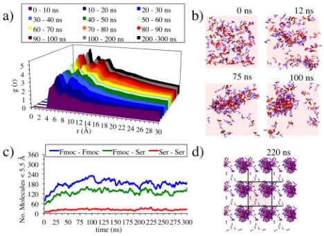
Fmoc-S-OH simulation results and comparison with experiment. The snapshots of the simulation show how after 220 ns the Fmoc-S-OH form a spherical aggregate (Figure 7d), which is consistent with the experimental results.

The radial distribution functions for the first 100 ns are calculated by taking snapshots of the systems every 0.01 ns (i.e., 1000 frames per 10 ns), whereas for the distributions from 100 – 300 ns are based on snapshots of the system taken every 0.1 ns (i.e. 1000 frames per 100 ns). The lower sampling frequency in the latter stages of the simulation was due to the relative stability of the system after 100 ns.

The RDF analysis (Figure 7a) shows three distinctly different sizes of aggregates through the simulation: peak 1

formation of a spherical aggregate (Figure 7b, 100ns). A fourth and a fifth peak around 12 – 16 Å and 16 – 20 Å, respectively, is also observed in the equilibrated parts of the graph.

The higher peak 3 between 80 and 100 ns in comparison with the 100 – 300 ns results could be due to an elongation of the aggregated spheres to an ellipse like aggregate. However, as the simulation continues and is averaged over longer timescales, this elongation effect is no longer present.

In the proximity analysis (Figure 7c), due to the different size of the groups analysed, it is difficult to compare the relative importance of the role of the contacts studied. However, the Ser – Ser contacts are mostly negligible through the whole simulation with a maximum value 35, which is equivalent to ~0.3 interactions/molecule, while the Fmoc – Fmoc and Fmoc – Ser reach maxima of ~1.9 and ~1.3 respectively. This suggests that the Ser groups tend to be exposed to the solvent, forming H-bonds, instead of interacting with other Ser groups.

The proximity analysis (Figure 7c) shows a rapid increase in the Fmoc – Fmoc proximity as well as the Fmoc – Ser proximity, which is likely due to the arrangement achieved through the Fmoc π-stacking interactions. The proximity analysis reveals how the molecules aggregate quickly in the first 25 ns to relatively stable structures, until ~50 ns, where the aggregation is seen to increase further. This is in good agreement with the RDF analysis, which shows an early aggregation step at the same time of the simulation. Once the small aggregates are formed they coalesce to form larger aggregates (50 – 100 ns). Therefore, the Fmoc – Fmoc interactions remain constant while peak 2 of the RDF increases (Figure 7a). This suggests that this increase is not due to Fmoc interactions, which are mostly buried in the small aggregates, but once these small aggregates join, the Fmoc groups of the aggregates interact inside the larger aggregate (as peak 1 in the RDF at 50 to 100 ns). The highest level of Fmoc – Fmoc aggregation is reached around 100 ns. This high number of interactions slightly decreases, in a process of equilibrating the aggregate, and remains relatively unchanged, apart from normal fluctuations, at ~180 Fmoc - Fmoc interactions (~1.5 interactions/molecule) from 110 – 300 ns forming and aggregate around 40 Å.

Although specific interactions are not determined in detail, the proximity analysis can be used to identify the orientations of the Fmoc – Fmoc systems (Figure 4) that most closely correlate with the simulations results. All of the orientations are expected to have a high number of Fmoc – Fmoc interactions and hence, the other two parameters provide more insight, using the former as a reference. The Ser – Ser interactions are negligible and hence, parallel stacking orientations can be excluded. In contrast, the number of Fmoc – Ser interactions is similar to that of the Fmoc – Fmoc interactions, which suggest that T forms are also not dominant in the simulation. Therefore, a dominant non-T antiparallel orientation most readily explains the proximity analysis results. The AFM image of Fmoc-S-OH published by Abul-Haija et al.4 shows many small aggregates and only a few larger ones, but not aggregates of intermediate size. While care should be

taken with the interpretation of AFM images because of possible drying effects influencing the size distribution, the mechanism observed in the simulation reveals how these larger aggregates are formed when many small aggregates coalesce, which is consistent with this experimental observation. Furthermore, the simulation is also in good agreement with the shape of the aggregates, which are mostly spherical, with a limited number showing a degree of ellipticity. However, in addition to this data, the simulation of the Fmoc-S-OH system also provides insight into which interactions are driving the different stages of the process. That is, the initial formation of the small aggregates is driven by the π-stacking interactions of the Fmoc moieties, followed by the H-bonding interactions between the Ser-OH moieties which allow the small aggregates to come together to finally be stabilized through additional π-stacking between the Fmoc moieties. Therefore, in addition to the simulation providing good agreement with the experimental results it also is able to contribute unique insights into the molecular level information, which is otherwise inaccessible experimentally.

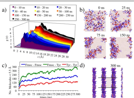
Fmoc-Y-OH simulation results and comparison with experiment. This simulation requires up to 300 ns to reach an equilibrated structure (Figure 8d). For this simulation, the RDFs are calculated every 0.01 ns for the first 50 ns (i.e., 1000 frames per 10 ns) and every 0.05 for the rest of the simulation (i.e., 1000 frames per 50 ns).

The RDF analysis of Fmoc-Y-OH (Figure 8a) is similar to the Fmoc-S-OH (Figure 7a) for the first 10 ns, showing three peaks of similar intensity, where peak 1 (3.5 – 7 Å) is dominant due to the first stages of aggregation between Fmoc-Y-OH molecules. After the first 10 ns of the simulation, peak 3 (9 – 12 Å) increases faster than peak 2 (7 – 9 Å), in contrast to Fmoc-S-OH, due to the elongated nature of the aggregates forming (Figure 8b, 25 ns). Between 40 ns and 150 ns both peaks are of similar intensity, while peak 1 clearly decreases, corresponding to the formation of a fibre like structure from the aggregates (Figure 8b, 75ns and 150 ns). At the end of the

simulation peak 1 increases again but remains below peak 3

and peak 2, which is the highest peak (Figure 8a, grey and black). In the final 50 ns two additional peaks form around 12 – 16 Å and 16 – 20 Å. These peaks were also present in the Fmoc-S-OH simulations but they are clearly more prominent in the last 50 ns of the Fmoc-Y-OH simulation. This is consistent with the formation of a more ordered, equilibrated fibre observed at the end of the simulation (Figure 8d).

The Fmoc-Y-OH proximity analysis (Figure 8c) shows a rapid increase in the three proximity curves during the first 10 ns of the simulation. This can be attributed to the fast aggregation of the aromatic groups of both, the Fmoc and the Tyr. This increment at the start is faster than in the case of Fmoc-S-OH. In addition, the amino acid – amino acid proximity (Tyr – Tyr), unlike in the case of the Ser – Ser, is of importance, reaching an averaged 120 proximity counts over the last 100 ns of the simulation. These two effects are caused by the hydrophobicity of the tyrosine side chain and its ability to form π-stacking interactions. Despite the fact that the initial aggregation occurs more rapidly, relative to Fmoc-S-OH, the proximity curves continue to increase throughout the simulation, which shows that the more complex fibre structure requires more time to equilibrate than the simple spherical aggregate of Fmoc-S-OH. The Fmoc – Fmoc proximity values are similar to those for the Fmoc-S-OH (~180), but the interactions that involve the Tyr are much more significant than the analogous interactions involving Ser: Fmoc – Ser reaches ~120, while Fmoc – Tyr, ~360; Ser – Ser interactions equilibrate at ~25 whereas Tyr – Tyr are ~120. This clearly shows the importance of the aromatic side chain in forming fibres rather than spherical aggregates.

The important role of the three types of interactions identified with the proximity analysis (Figure 8c) makes it difficult to relate the results with the Fmoc – Fmoc orientations studied before (Figure 4), as was done for the Fmoc-S-OH system. This is because the arrangement of simple dimers cannot explain the abundance of the three types of interactions as these probably arises from interactions between multiple molecules (e.g., twisted-stacks).

The ability to reproduce two different experimentally known nanostructures from closely related systems clearly demonstrates that the parameterization has achieved the correct balance and description of the important interactions to correctly describe the role of Fmoc in forming these different nanostructures.

Conclusions

A new protocol for the parameterization of amphiphilic molecules to be used in self-assembling studies has been developed. A set of parameters for the Fmoc moiety has been derived for the CHARMM force field using this protocol. The parameters are shown to be able to reproduce intermolecular interactions by reproducing QM binding energies between the moiety and water and between two Fmoc moieties, and to reproduce the flexibility of the Fmoc group by comparing

energetic profile with the corresponding QM dihedral scans. Furthermore, the Fmoc parameterization presented in this paper has successfully reproduced thermodynamic parameters directly related to the self-assembling behaviour and experimental results involving self-assembling of the moiety linked to an amino acid. This includes achieving different nanostructures for different systems, spheres for Fmoc-S-OH and fibres for Fmoc-Y-OH, consistent with the experimental findings for these systems. The validity of the parameters supports the modifications made in the protocol for this type of molecule and suggest a new procedure for the future parameterization of other amphiphilic moieties.

Acknowledgements

The authors gratefully acknowledge the financial support by the EC 7th Framework Programme Marie Curie Actions via the European ITN SMARTNET No. 316656 and EMERgE/ERC No. 258775. Results were obtained using the EPSRC funded ARCHIE-WeSt High Performance Computer (www.archie-west.ac.uk). EPSRC grant no. EP/K000586/1.

References

1. M. Zelzer and R. V. Ulijn, Chem. Soc. Rev., 2010, 39, 3351-3357.

2. G. M. Whitesides and B. Grzybowski, Science, 2002, 295, 2418-2421.

3. J. E. Gough, A. Saiani and A. F. Miller, Bioinspired, Biomimetic and Nanobiomaterials, 2011, 1, 4-12.

4. Y. M. Abul-Haija, S. Roy, P. W. Frederix, N. Javid, V. Jayawarna and R. V. Ulijn, Small, 2014, 10, 973-979. 5. M. Hughes, L. S. Birchall, K. Zuberi, L. A. Aitken, S.

Debnath, N. Javid and R. V. Ulijn, Soft Matter, 2012, 8, 11565-11574.

6. M. Reches and E. Gazit, Science, 2003, 300, 625-627. 7. M. Hughes, P. W. J. M. Frederix, J. Raeburn, L. S. Birchall,

J. Sadownik, F. C. Coomer, I. H. Lin, E. J. Cussen, N. T. Hunt, T. Tuttle, S. J. Webb, D. J. Adams and R. V. Ulijn, Soft Matter, 2012, 8, 5595-5602.

8. Y. R. Zhao, J. Q. Wang, L. Deng, P. Zhou, S. J. Wang, Y. T. Wang, H. Xu and J. R. Lu, Langmuir, 2013, 29, 13457-13464.

9. M. McCullagh, T. Prytkova, S. Tonzani, N. D. Winter and G. C. Schatz, J. Phys. Chem. B, 2008, 112, 10388-10398. 10. Y. S. Velichko, S. I. Stupp and M. O. de la Cruz, J. Phys.

Chem. B, 2008, 112, 2326-2334.

11. O.-S. Lee, V. Cho and G. C. Schatz, Nano Lett., 2012, 12, 4907-4913.

12. T. Yu and G. C. Schatz, J. Phys. Chem. B, 2013, 117, 14059-14064.

13. P. W. J. M. Frederix, R. V. Ulijn, N. T. Hunt and T. Tuttle, J. Phys. Chem. Lett., 2011, 2, 2380-2384.

14. P. Frederix, W. J. M., G. G. Scott, Y. M. Abul-Haija, D. Kalafatovic, C. G. Pappas, N. Javid, N. T. Hunt, R. V. Ulijn and T. Tuttle, Nature Chem., 2015, 7, 30-37.

16. O.-S. Lee, Y. Liu and G. C. Schatz, J. Nanopart. Res., 2012, 14, 1-7.

17. O.-S. Lee, S. I. Stupp and G. C. Schatz, J. Am. Chem. Soc., 2011, 133, 3677-3683.

18. T. Yu and G. C. Schatz, J. Phys. Chem. B, 2013, 117, 9004-9013.

19. T. Yu, O. S. Lee and G. C. Schatz, J. Phys. Chem. A, 2013, 117, 7453-7460.

20. R. Orbach, L. Adler-Abramovich, S. Zigerson, I. Mironi-Harpaz, D. Seliktar and E. Gazit, Biomacromolecules, 2009, 10, 2646-2651.

21. J. D. Hartgerink, E. Benlash and S. L. Stupp, Science, 2001, 294, 1684-1688.

22. F. Versluis, H. R. Marsden and A. Kros, Chem. Soc. Rev., 2010, 39, 3434.

23. R. V. Ulijn and A. M. Smith, Chem. Soc. Rev., 2008, 37, 664-675.

24. C. Tang, R. V. Ulijn and A. Saiani, Langmuir, 2011, 27, 14438-14449.

25. C. Tang, R. V. Ulijn and A. Saiani, Eur. Phys. J. E, 2013, 36, 1-11.

26. M. Caruso, E. Gatto, E. Placidi, G. Ballano, F. Formaggio, C. Toniolo, D. Zanuy, C. Alemán and M. Venanzi, Soft Matter, 2014, 10, 2508-2519.

27. Z. Yang, H. Gu, D. Fu, P. Gao, J. K. Lam and B. Xu, Adv. Mater, 2004, 16, 1440-1444.

28. S. Sutton, N. L. Campbell, A. I. Cooper, M. Kirkland, W. J. Frith and D. J. Adams, Langmuir, 2009, 25, 10285-10291. 29. S. Fleming and R. V. Ulijn, Chem. Soc. Rev., 2014, 43,

8150-8177.

30. S. Fleming, S. Debnath, P. W. J. M. Frederix, T. Tuttle and R. V. Ulijn, Chem. Commun., 2013, 49, 10587-10589. 31. X. J. Mu, K. M. Eckes, M. M. Nguyen, L. J. Suggs and P. Y.

Ren, Biomacromolecules, 2012, 13, 3562-3571.

32. H. X. Xu, A. K. Das, M. Horie, M. Shaik, A. M. Smith, Y. Luo, X. Lu, R. Collins, S. Y. Liem, A. Song, P. L. A. Popelier, M. L. Turner, P. Xiao, I. A. Kinloch and R. V. Ulijn, Nanoscale, 2010, 2, 960-966.

33. V. Castelletto, C. Moulton, G. Cheng, I. Hamley, M. R. Hicks, A. Rodger, D. E. López-Pérez, G. Revilla-López and C. Alemán, Soft Matter, 2011, 7, 11405-11415.

34. A. Mackerell, D. Bashford, M. Bellot, R. Dunbrack, J. Evanseck, M. Field, J. Gao, H. Guo, S. Ha, D. Joseph -McCarthy, L. Kuchnir, K. Kuczera, F. T. K. Lau, C. Mattos, S. Michnick, T. Ngo, D. T. Nguyen, B. Prodhom, W. E. E. Reiher, B. Roux, M. Schlenkrich, J. C. Smith, R. Stote, J.

Straub, M. Watanabe, J. Wio ́rkiewicz-Kuczera, D. Yin and M. Karplus, J. Phys. Chem. B, 1998, 102, 3586.

35. A. R. Leach, Molecular modelling: principles and applications, Prentice Hall, Harlow [etc.], 2001.

36. S. A. Adcock and J. A. McCammon, Chem. Rev., 2006, 106, 1589-1615.

37. W. F. van Gunsteren, D. Bakowies, R. Baron, I. Chandrasekhar, M. Christen, X. Daura, P. Gee, D. P. Geerke, A. Glättli and P. H. Hünenberger, Angew. Chem., 2006, 45, 4064-4092.

38. B. R. Brooks, C. L. B. III, A. D. M. Jr, L. Nilsson, R. J. Petrella, B. Roux, Y. Won, G. Archontis, C. Bartels, S. Boresch, A. Caflisch, L. Caves, Q. Cui, A. R. Dinner, M. Feig, S. Fischer, J. Gao, M. Hodoscek, W. Im, K. Kuczera, T. Lazaridis, J. Ma, V. Ovchinnikov, E. Paci, R. W. Pastor, C. B. Post, J. Z. Pu, M. Schaefer, B. Tidor, R. M. Venable, H. L. Woodcock, X.

Wu, W. Yang, D. M. York and M. Karplus, J. Comput. Chem., 2009, 30, 1545-1614.

39. A. D. MacKerell, N. Banavali and N. Foloppe, Biopolymers, 2000, 56, 257–265.

40. K. Vanommeslaeghe, E. Hatcher, C. Acharya, S. Kundu, S. Zhong, J. Shim, E. Darian, O. Guvench, P. Lopes, I. Vorobyov and A. D. Mackerell, J. Comput. Chem., 2010, 31, 671–690.

41. E. T. Prates, P. C. Souza, M. Pickholz and M. S. Skaf, Int. J. Quantum Chem., 2011, 111, 1339-1345.

42. A. Hansson, P. C. Souza, R. L. Silveira, L. Martinez and M. S. Skaf, Int. J. Quantum Chem., 2011, 111, 1346-1354. 43. S. Grimme, J. Comput. Chem., 2006, 27, 1787-1799. 44. A. Schäfer, H. Horn and R. Ahlrichs, J. Chem. Phys., 1992,

97, 2571-2577.

45. TURBOMOLE, 6.3.1 (2012), TURBOMOLE GmbH.

46. R. Ahlrichs, M. Bär, M. Häser, H. Horn and C. Kölmel,

Chem. Phys. Lett., 1989, 162, 165-169.

47. J. C. Phillips, R. Braun, W. Wang, J. Gumbart, E. Tajkhorshid, E. Villa, C. Chipot, R. D. Skeel, L. Kalé and K. Schulten, J. Comput. Chem., 2005, 26, 1781–1802. 48. W. L. Jorgensen, J. Chandrasekhar, J. D. Madura, R. W.

Impey and M. L. Klein, J. Chem. Phys., 1983, 79, 926-935. 49. M. D. Hanwell, D. E. Curtis, D. C. Lonie, T. Vandermeersch,

E. Zurek and G. R. Hutchison, J. Cheminform., 2012, 4, 17. 50. Gaussian 09, (2009), Gaussian, Inc.

51. A. D. Becke, The Journal of Chemical Physics, 1993, 98, 5648-5652.

52. C. Lee, W. Yang and R. G. Parr, Physical Review B, 1988, 37, 785.

53. W. J. Hehre, R. Ditchfield and J. A. Pople, The Journal of Chemical Physics, 1972, 56, 2257-2261.

54. P. C. Hariharan and J. A. Pople, Theor. Chim. Acta, 1973, 28, 213-222.

55. J. Sangster, J. Phys. Chem. Ref. Data, 1989, 18, 1111-1229. 56. K. B. Lodge, J. Chem. Eng. Data, 1999, 44, 1321-1324. 57. D. J. Edelbach and K. B. Lodge, Phys. Chem. Chem. Phys.,

2000, 2, 1763-1771.

58. R. W. Zwanzig, J. Chem. Phys., 1954, 22, 1420-1426. 59. R. W. Zwanzig, J. Chem. Phys., 1955, 23, 1915-1922. 60. W. Humphrey, A. Dalke and K. Schulten, J. Mol. Graphics,

1996, 14, 33-38.

61. O. N. de Souza and R. L. Ornstein, Biophys. J., 1997, 72, 2395-2397.

62. S. E. Feller, Y. Zhang, R. W. Pastor and B. R. Brooks, J. Chem. Phys., 1995, 103, 4613-4621.

63. N. Bhatnagar, G. Kamath, I. Chelst and J. J. Potoff, J. Chem. Phys., 2012, 137.

64. T. C. Beutler, A. E. Mark, R. C. van Schaik, P. R. Gerber and W. F. van Gunsteren, Chem. Phys. Lett., 1994, 222, 529-539.

65. J. W. Pitera and W. F. van Gunsteren, Mol. Simul., 2002, 28, 45-65.

66. C. Chipot and A. Pohorille, Free energy calculations, Springer, 2007.

67. C. Lee and H. Scott, J. Chem. Phys., 1980, 73, 4591-4596. 68. P. Liu, F. o. Dehez, W. Cai and C. Chipot, J. Chem. Theory