Multiple mortality modeling in Poisson Lee-Carter framework

City, University of London Institutional Repository

Citation

:

Multiple mortality modeling in Poisson Lee-Carter framework. Communications in Statistics - Theory and Methods, 45(6), pp. 1723-1732. doi: 10.1080/03610926.2014.960580

This is the accepted version of the paper.

This version of the publication may differ from the final published

version.

Permanent repository link:

Link to published version

:

Copyright and reuse:

City Research Online aims to make research

outputs of City, University of London available to a wider audience.

Copyright and Moral Rights remain with the author(s) and/or copyright

holders. URLs from City Research Online may be freely distributed and

linked to.

City Research Online: http://openaccess.city.ac.uk/ [email protected]

ACCEPTED MANUSCRIPT

Multiple Mortality Modeling in Poisson Lee Carter framework

Valeria D'Amato1, Steven Haberman2,Gabriella Piscopo3, Maria Russolillo1 and

Lorenzo Trapani2

1

Department of Economics and Statistics, University of Salerno, via Ponte Don Melillo, Campus

Universitario, 84084 Fisciano (Salerno), Italy

e-mail: [email protected], [email protected]

2

Faculty of Actuarial Science and Insurance, Cass Business School, City University, Bunhill

Row London, UK, e-mail: [email protected]

3

Department of Economics, University of Genoa, Via Vivaldi, 16126 Genoa, Italy - e-mail:

[email protected]

Abstract

The academic literature in longevity field has recently focused on models for detecting multiple

population trends (D'Amato et al. 2012b, Nijenga et al. 2011, Russolillo et a. 2011, etc.). In

particular increasing interest has been shown about “related” population dynamics or “parent”

populations characterized by similar socio-economic conditions and eventually also by

geographical proximity. These studies suggest dependence across multiple populations and

common long run relationships between countries (for instance see Lazar et al. 2009). In order to

investigate cross-country longevity common trends, we adopt a multiple population approach.

ACCEPTED MANUSCRIPT

The algorithm we propose retains the parametric structure of the Lee Carter model, extending the

basic framework to include some cross dependence in the error term. As far as time dependence

is concerned, we allow for all idiosyncratic components (both in the common stochastic trend

and in the error term) to follow a linear process, thus considering a highly flexible specification

for the serial dependence structure of our data. We also relax the assumption of normality, which

is typical of early studies on mortality (Lee and Carter, 1992) and on factor models (see e.g. the

textbook by Anderson, 1984). The empirical results show that the Multiple Lee Carter Approach

works well in presence of dependence.

Keywords

Serial and Cross-sectional Correlation, Factor Models, Vector Auto-Regression, Sieve Bootstrap,

Lee Carter model

ACCEPTED MANUSCRIPT

1Introduction

The whole financial system is dramatically threatened by the systematic improvements in

longevity phenomenon, especially regarding the welfare and public pensions. The empirical

evidence shows the presence of common factors that would affect survival rates across multiple

populations in a similar way. The reason behind is that populations of the world are becoming

more closely linked by communication, transportation, trade, technology, and disease.

Modeling mortality co-movements for multiple populations would have significant implications

for longevity risk management.

In a multi-population mortality model, the analysis is focused on more than one population by

taking into account a joint framework. The main idea behind these models lies on the

convergence indefinitely over time observed between populations having similar socioeconomic

features. The development of multiple setting is related to the several applications. First of all,

securitization of longevity risk, i.e. the transfer of longevity risk in the capital markets, which

typically occurs through the creation of derivatives or securities whose cash flows are linked to

the survival of a reference population, a more effective risk management can be obtained

throughout the study of the mortality correlations between populations. The relationship between

populations is involved in the estimation of the actual basis risk which arises from the difference

in mortality improvements between the insured population and the population to which the

standardized longevity hedging instruments are linked. Hedging instruments have been

developed in order to help pension funds to protect themselves against longevity risk, in

particular by reinsurance and longevity derivatives.

ACCEPTED MANUSCRIPT

Secondly the multiple population mortality model allows for enhancing the estimate reliability

by modeling the smaller population jointly with a larger population (Li et al. 2010).

Furthermore the multiple approach can also be used for enforcing greater consistency of the sex

differentials when an analysis on both genders has to be performed.

Recently, significant developments in multi-population modeling have been recorded.

The seminal interest in studying cross-country longevity common trends focused on modeling

the interdependence of the mortality rates of two populations. Li and Lee (2005) developed an

augmented common factor model for modeling convergent mortality dynamics. Li et al. (2011)

propose a model that measures the population basis risk involved in a longevity hedge. Cairns et

al. (2011) represents the short trends by using a mean-reverting spread, where the long-run

improvements are parallel according to biological principle. Jarner et al. 2011 develop a similar

two-step approach modeling the mortality of larger reference population and the mortality spread

between the two populations. The current studies investigate on long-run equilibrium

relationships across countries, by considering the more than two populations in the mortality

framework, for capturing valuable information about the factors driving changes in mortality

(Njienga et al., 2011; Russolillo et al., 2011). Other authors model mortality dependence

(structure) across countries using a dynamic copula approach (Yang et al. 2013). In particular,

they employ time-varying copula introducing mortality dependence and demonstrate symmetric

dependence. In the same context MacMinn et al. 2013 are the first to apply the factor copula

model to mortality fitting for multiple populations. They focus on the residual risk (tail

dependence) by setting out an efficient approach for high dimensional data. Kleinow (2013)

ACCEPTED MANUSCRIPT

shows that the period effects of different populations in a CAE model are better comparable with

each other since the impact of different age effects is eliminated. This aspect can be relevant in

effectiveness of hedge positions.

In order to study cross-country longevity common trends, it is essential to consider tools to

quantify, compare and model the strength of dependence. Therefore it is necessary to take into

account either the dependence for adjacent age groups, or the dependence structure across time

in a single population setting: a sort of intra-dependence structure (D'Amato et al. 2012b). At the

same time, it is important to consider the dependence across multiple populations, what we call

inter-dependence, for capturing common long run relationships between countries.

In a previous contribution (D'Amato et al. 2013), we kept into account the issue of

cross-sectional and time dependence, by proposing an algorithm based on the Lee Carter framework

(1992), but relaxing the assumption of normality, which is typical of early studies on mortality

(Lee and Carter, 1992) and on factor models (see e.g. the textbook by Anderson, 1984). In this

article, we extend that formulation by taking into consideration a different fitting model for

mortality data, the Poisson log-bilinear mortality model, which allows to overcome the problems

associated with the OLS method in the fitting procedure.

We also consider a bootstrap procedure for dependent data, thus preserving both the historical

parametric structure and the intra-group error correlation structure. In particular, we apply a

Sieve bootstrap algorithm (Bulhmann, 1997) to the Vector AutoRegression (VAR henceforth)

model containing the estimated common factors (both stationary and non-stationary). However,

in a previous paper (D'Amato et al. 2012b), we stated that in our context we cannot apply a

ACCEPTED MANUSCRIPT

standard Sieve bootstrap algorithm, since, when resampling the estimated common factors, a

generated regressors problem arises. In this order of ideas, our paper is based on Trapani (2012),

which develops the full blown theory to apply Sieve bootstrap to the context of non-stationary

panel factor series, developing selection rules for the order of the VAR and showing the superior

performance of Sieve bootstrap compared to first-order asymptotic. In particular, the paper is

structured as follows: Section 2 faces the issue of Multiple Alignment. In section 3, we present

the Poisson log-bilinear mortality model. Section 4 discusses the methodology to generate the

bootstrap sample by proposing the Multiple Poisson Lee Carter Panel Sieve Algorithm. Section 5

shows the results of the Numerical Application. Section 6 contains the Concluding Remarks.

2 Multiple Setting

The representation of multiple populations bases on similar mortality behaviours typical for

people which share analogous living conditions. Studying mortality experience for a group of

populations with similar mortality behaviours might improve the stability of mortality modelling

(Yang et al. 2011). Moreover it could allow for solving the problem of small population. Indeed

some authors propose the replication of the data by mixing appropriately the mortality data from

neighbouring countries (Olivieri 2011). The crucial point working with different populations is

that the dependence structure analyzed in previous works for a single dataset (D'Amato et al.,

2012a) becomes very complex and has to be taken into account under a multidimensional

approach. In fact, three kinds of dependence have to be captured: thecross sectional dependence

for adjacent age groups, across countries and serial/time dependence. In this case, the classical

Sieve bootstrap cannot be applied to the three-dimensional dataset, due to a too large number of

ACCEPTED MANUSCRIPT

cross-sectional units. D'Amato et al. 2013 originally solve this problem looking for a rational

reduction of the dataset. To this aim, they consider that the common trends between countries are

captured by the time-varying parameters k_t of the LC model and propose the following

alignment of the data (we refer to Lee and Carter, 1992 for a deepened description of the

parameters involved in the Lee- Carter method). They fit separately the LC on some mortality

dataset of M different populations, composed by the same ages xa a, 1, ,aN and years

, 1, ,

tb b b T , where a represents the first age, fixed equal to zero and b the first time,

respectively. N and T represents the last age and the length of the period considered,

respectively. Once they obtain the k_t’s for each country, they arrange the M time series of k_t in

a matrix, generating a panel data in which the single units are represented by the different

populations and are collected in rows. In this way, they obtain a reduced dataset on which it is

possible to design a Sieve bootstrap. The framework they propose is very flexible and lends itself

to interesting extensions and more accurate formulations. One of this is the possibility to take

into account a different fitting model for mortality data. An example could be the Poisson

log-bilinear mortality model, described in the next Section.

3 The Poisson log-bilinear mortality model

D'Amato et al. (2012) develop the idea of first fitting Lee Carter parametric model, and then

re-sampling a particular class of the residuals, the so-called centred residuals, according to the Sieve

scheme, through an autoregressive approximation for generating bootstrap replications of the

data. They firstly consider the Lee Carter parametric framework because of its well known

properties (Deaton and Paxson, 2004); however, this model making use of the least-square tool

ACCEPTED MANUSCRIPT

for mortality estimation is based on the hypothesis of homoskedastic errors, but this assumption

is not confirmed by the empirical evidence. Instead, the Poisson log-bilinear model allows to

overcome the problems associated with the OLS method in the fitting procedure. Because the

number of deaths is a counting random variable, according to Brillinger (1986), the Poisson

assumption appears to be plausible. It has been argued that the number of deaths, when the

central exposed-to-risk is given, may be assumed to follow a Poisson distribution. At the same

time the promising estimates may be obtained by fitting the Poisson regression (see Renshaw and

Haberman(1997), Renshaw et al (1996), and Sithole et al. (2000)):









, , , with , exp

x t x t x t x t x x t

D Poisson E    a b k (1)

where the parameters are still subjected to the constraints _t 0

t

k 



x

b 



mortality is thus assumed to have the log-bilinear form:

 

ln _{x t} a_xk b_{t x}. (2)

Recently the Poisson version of the Lee-Carter model has been deepened and applied in actuarial

literature. Some essential improvements have been introduced by Brouhns et al. (2002) who

estimate parameters by Poisson log-bilinear regression and Renshaw and Haberman (2003) who

describe the model in the GLM terms. In the light of this consideration, we exploit the Poisson

version of the Lee Carter model in the Panel Sieve bootstrap, as an extension of the model shown

in D'Amato et al. 2013, confirming the flexible nature of the algorithm presented in our previous

work.

ACCEPTED MANUSCRIPT

4. Algorithm: Multiple Poisson Lee Carter Panel Sieve

This section discusses the methodology to generate the bootstrap sample. The preliminary step is

the construction of matrix K through the fitting of the LC model on different populations

separately.

For each population i, we fit the Poisson version of the LC model according to eq. (1),

determining ˆk_ti. The parameters k_{t i,} are then arranged in a matrix KMXT. A VAR is fitted to this

matrix. The VAR is the statistical tool employed to represent how different populations are

related each other.

Let Kt = [k₁t′,…,kMt′]′ denote an (Mx1) vector of time series variables. The basic q-lag VAR(q)

has the form:

1

, 1,...,

q

t j t j t j

K A K_  t T







Where A is the matrix of coefficient of the selected VAR(q) model.

Hence the bootstrapping algorithm is as follows:

Step 1. (PC estimation)

(1.1)For each i, estimate the kt,i in (1).

(1.2)Arrange the fitted kt,i in the matrix K

Step 2. (VAR model estimation)

ACCEPTED MANUSCRIPT

(2.1) Estimate the matrix of coefficient Aof the VAR(q) model by applying OLS to (4). The q

lag selection criteria is the Akaike’s information criterion (AIC)

(2.2) Compute the residuals _{, ,}

1

ˆ ˆ ˆ

ˆ_{t q t} qK _{q j t j}

j

e k A k_



  



defining them e_{t q,} .

Step 3. (bootstrap) for b = 1,…,ℶ iterations

(3.1) (resampling)

(3.1.a) Draw (with replacement) T values from

 

1

T t q _t

e

 to obtain the bootstrap sample

 

T t b _t

e



(3.2) (generation of the bootstrap sample)

(3.2.a) Generate recursively the pseudo sample _{, , , ,}

1

ˆ

qK

t b q j t j b t b j

k A k_ e



 



(3.2.b) Generate kt,b as , 0, ,

1

t t b b j b

j

k k k



 



In this way we obtain b matix K_MXTb from which we can generate the pseudo sample

 

1

T b xt i _t





according to eq. (1).

5. Numerical Application

In the present section, we apply the methodology described in the section 4 to the historical

mortality data for five countries expected to have experienced common longevity improvements,

ACCEPTED MANUSCRIPT

on the basis of similar socio-economic features: United Kingdom (henceforth UK), France, Italy,

Spain and Belgium. The study is performed for each country on total population (composed by

male and female) ranging from 1950 to 2006, for ages from 0 up to 110 years, considered by

single calendar year and by single year of age, where the class of age above 100 years is

collected in an open age group 100+ (the data were downloaded from the Human Mortality

Database). The first step is the fitting of the Poisson version of the LC on the datasets of the five

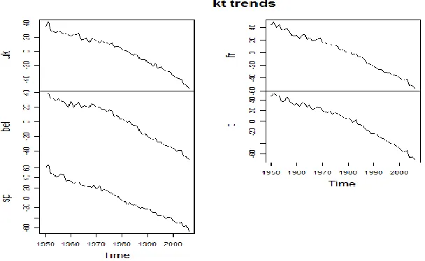
selected countries. In Figure 1, we show the estimates of the trend parameters for each country:

Observing Figure 1, we note that the estimated trends of the parameter kt are quite similar for

each country, showing wherever a decreasing slope. We refer to D'Amato et al. 2013 for a

detailed description of similarities and measurement of dependence in mortality between the

selected countries.

In the second step of this numerical application, we fit the VAR model to the k_t of each country

and calculate the residuals. The number of lags of the VAR model is selected through the

application of the Akaike criterion, useful to avoid the overparameterisation of the model. The

result is that the selected lagged terms are two so that each lag term Kt-q,mi for country i affect

the response Kt,mj with i = j and i≠j, q = 1,2. In other words, not only own country lags are

relevant, but each country influences the response of the others for two legs.

Figures 2-6 display, for each country, a diagram of fit, a residual plot, the auto-correlation and

partial auto-correlation function of the residuals.

Finally, we have implemented the bootstrap simulation according to the algorithm proposed in

ACCEPTED MANUSCRIPT

sample average k_t. Then, we have projected them by using ARIMA models and calculated

confidence intervals. Figures 7 displays the mean of the simulated k_t and the projections with

confidence intervals for UK, Belgium, Spain, France and Italy.

In Figure 7, the solid lines represent the kt trend for UK, Belgium, Spain, France and Italy, with

the confidence intervals highlighted in yellow. As it is clear by the diagrams, the trend is quite

similar between countries, that have experienced similar trends in mortality reduction due to

common social-economic factors and improvements in medical research. But if we look at the

width of the confidence intervals, we can see they are quite unequal between countries. In

particular, as result of our application it is relevant to notice the wider CI’s for Belgium, which is

the smallest of the considered countries. In the Introductin we stated that by considering a

multiple model we allow enhancing the reliability for small population mortality estimates. In

other words, the knowledge about countries with small population can be enriched by the

consideration of common features between different populations.

Further research will aim to verify the forecast goodness of the Multiple Lee Carter Approach

throughout different measures of forecast accuracy, also to test the improvement of the proposed

model with respect to the classical Lee Carter model.

6. Concluding Remarks

In the last few years there has been an increasing interest in the actuarial literature on the issue of

modeling multiple populations characterized by similar socio-economic and living conditions. It

has also been shown the problems arising when considering simultaneously different countries is

ACCEPTED MANUSCRIPT

strictly related to the dependence analysis. The existence of dependence in mortality data

involves the interactions for adjacent age groups between age and time and also across the

different populations.

From a methodological point of view, the research presented in this contribution is oriented to

consider the flexibility of the methodology proposed in a previous article (D'Amato et al. 2013).

In particular, we build on the Lee Carter method in its Poisson version to develop an approach

within this general framework. In particular, we extend the basic structure to include some cross

dependence in the error term on the basis of a tailor-made bootstrap algorithm, explained in

detail in section 4.

Another attractive methodology for our application could have been Bayesian (empirical, full)

with the kti as random effects. Bayesian simulation differs from classical simulation analysis in

that probability distributions are used to represent the uncertainty about model parameters, rather

than point estimates and confidence intervals. In the Bayesian approach, the prior information

about the distribution of parameters is modified into posterior one after the observation of

sample. In the language of uncertainty, classical simulation models only aleatory uncertainty (the

randomness of the system itself), while Bayesian simulation models both the aleatory and

epistemic uncertainty (the lack of knowledge about the system). However, as it has been

observed (Hastie et al., The Elements of Statistical Learning 2009) “bootstrap distribution

represents an approximate non-parametric posterior based on a particular choice of

noninformative prior … and is typically much simpler to carry out.” In other words, referring to

our case the prior from which we start is the fitted kt from the model and the bootstrap algorithm

ACCEPTED MANUSCRIPT

approximate the posterior information about the distribution of the parameter offering point

estimates and confidence intervals; in this way we reach a quicker results than that we should

obtain with Bayesian simulation. In actuarial application, it is important to reduce the time of

simulation to make really applicable the algorithm for practical uses; moreover, for practitioners

the quantities of interest are just the confidence intervals to estimates the impact of longevity risk

on insurance liabilities.

ACCEPTED MANUSCRIPT

References

1. Anderson, T. W., 1984, An Introduction to Multivariate Statistical Analysis, 2nd Edition, New

York: Wiley

2. Bai, J., 2004, Estimating cross-section common stochastic trends in nonstationary panel data,

Journal of Econometrics, 122, 137-183

3. Bühlmann, P., 1997, Sieve bootstrap for time series, Bernoulli, 3, 123-148

4. Cairns, A.J.G., D. Blake, K. Dowd, G.D. Coughlan, M. Khalaf-Allah, 2011, Bayesian

Stochastic Mortality Modelling for Two Populations. ASTIN Bulletin, 41(1), 29--59.

5. D'Amato V., Haberman S., Piscopo G., Russolillo M., 2013, Computational Framework for

Longevity Risk Management, Computational Management Science, DOI

10.1007/s10287-013-0178-2, Print ISSN 1619-697X, Online ISSN 1619-6988

6. D'Amato V., Haberman S., Piscopo G., Russolillo M., Trapani L., 2012b, Detecting longevity

common trends by a multiple population approach, presented at Eight International Longevity

Risk and Capital Market Solutions Conference, Waterloo, Ontario (CANADA)

7. D'Amato V., Haberman S., Russolillo M., 2012a, The Stratified Sampling Bootstrap: an

algorithm for measuring the uncertainty in forecast mortality rates in the Poisson Lee-Carter

setting. Methodology and Computing in Applied Probability, 14(1), 135-148.

ACCEPTED MANUSCRIPT

8. D'Amato V., Di Lorenzo E., Haberman S., Russolillo M., Sibillo M., 2011, The Poisson

log-bilinear Lee Carter model: Applications of efficient bootstrap methods to annuity analyses. North

American Actuarial Journal, 15(2), 315-333.

http://www.soa.org/library/journals/north-american-actuarial-journal/2011/no-2/naaj-2011-vol15-no2.aspx

9. D'Amato V., Haberman S., Piscopo G., Russolillo M., 2012b, Modelling dependent data for

longevity projections. Insurance Mathematics and Economics 51, 694-701, DOI information:

10.1016/j.insmatheco.2012.09.008

10. Dowd, K., Cairns, A.J.G., Blake, D., Coughlan, G.D., Epstein, D. and Khalaf-Allah, M.,

2011, A Gravity Model of Mortality Rates for Two Related Populations. North American

Actuarial Journal 15: 334-356.

11. Gaille S., Sherris M., 2011, Modelling Mortality with Common Stochastic Long-Run Trends.

The Geneva Papers on Risk and Insurance - Issues and Practice, 36(4), 595-621.

12. Guillen, M., Vidiella-I-Anguera, A., 2005, Forecasting Spanish natural life expectancy, Risk

Analysis, 25 (5), 1161-1170.

13. Hastie, T., Tibshirani, R., Friedman, J., 2009, The elements of statistical learning: data

mining, inference and prediction. Springer. (Chapter 2)

14. Human Mortality Database. University of California, Berkeley (USA) and Max Planck

Institute for Demographic Research (Germany). Available at www.mortality.org or

ACCEPTED MANUSCRIPT

15. Jarner S. F, Kryger E.M., 2011, Modelling Adult Mortality in a Small Population: The

SAINT model, Astin Bulletin 41 (2), p. 377-418

16. Kleinow T., 2013, A Common Age Effect Model for the Mortality of Multiple Populations,

paper presented at Ninth International Longevity Risk and Capital Markets Solutions

Conference, China

17. Lee, R.D., L. R. Carter, 1992, Modelling and Forecasting U.S. Mortality. Journal of the

American Statistical Association, 87, 659-671.

18. Li, N., R. Lee, 2005, Coherent mortality forecasts for a group of populations: An extension

of the Lee-Carter method. Demography, 42(3), 575--594.

19. Li, J.S.H., Hardy, M.R. and Tan, K.S. (2010). Developing Mortality Improvement Formulae:

The Canadian Insured Lives Case Study. North American Actuarial Journal 14: 381-399.

20. Li, J. S. H., Hardy, M. R., 2011, Measuring Basis Risk Involved in Longevity Hedges. North

American Actuarial Journal, 15(2), 177--200.

21. MacMinn R., Sun T., Chen H., 2013, A Multi-Population Mortality Model via the Factor

Copula Approach, paper presented at Ninth International Longevity Risk and Capital Markets

Solutions Conference, China

22. Njenga C., Sherris M., 2011, Longevity Risk and the Econometric Analysis of mortality

trends and volatility, Asia-Pacific Journal of Risk and Insurance, vol. 5, issue 2. 23. Olivieri A.,

2011, Forecasting mortality by mixing mortality experiences, Demography and Longevity

ACCEPTED MANUSCRIPT

24. Ornelas, A., Guillén, M., 2013, A comparison between general population mortality and life

tables for insurance in Mexico under gender proportion inequality, Revista de Metodos

Cuantitativos para la Economia y la Empresa, 16 (1), 47-67.

25. Russolillo, M., Giordano, G., Haberman, S., 2011, Extending the Lee-Carter model: a

three-way decomposition. Scandinavian Actuarial Journal, 2, 96-117.

26. Trapani, L., 2012, On bootstrapping panel factor series - Extended version. Available at

SSRN: http://ssrn.com/abstract = 2062183

27. Trapani, L., 2013, On bootstrapping panel factor series. Journal of Econometrics, 172,

127-141.

28. Yang S., Yue J.C., Yeh Y., 2011, Coherent Mortality Modeling for a Group of Populations,

Living to 100 Symposium.

29.Yang S.S., Huang H.C., Wang C., 2013, Modeling Multi-Country Mortality Dependence and

Its Application in Pricing Survivor Swaps: A Dynamic Copula Approach, paper presented at

Ninth International Longevity Risk and Capital Markets Solutions Conference, China

ACCEPTED MANUSCRIPT

Figure 1-Estimated trends of parameters kt

ACCEPTED MANUSCRIPT

Figure 2-Diagram of fit, residuals, ACF and PACF of residuals for UK

ACCEPTED MANUSCRIPT

Figure 3-Diagram of fit, residuals, ACF and PACF of residuals for France

ACCEPTED MANUSCRIPT

Figure 4-Diagram of fit, residuals, ACF and PACF of residuals for Belgium

ACCEPTED MANUSCRIPT

Figure 5-Diagram of fit, residuals, ACF and PACF of residuals for Spain

ACCEPTED MANUSCRIPT

Figure 6-Diagram of fit, residuals, ACF and PACF of residuals for Italy

ACCEPTED MANUSCRIPT

Figure 7- mean of simulated kt and projections for UK, Belgium, Spain, France and Italy