Complexity and Search Space Reduction in
Cyclic-by-Row PEVD Algorithms
Fraser K. Coutts
∗, Jamie Corr
∗, Keith Thompson
∗, Stephan Weiss
∗, Ian K. Proudler
∗,†, John G. McWhirter
‡ ∗ Department of Electronic & Electrical Engineering, University of Strathclyde, Glasgow, Scotland∗,† School of Electrical, Electronics & Systems Engineering, Loughborough Univ., Loughborough, UK
‡ School of Engineering, Cardiff University, Cardiff, Wales, UK
{fraser.coutts,jamie.corr,keith.thompson,stephan.weiss}@strath.ac.uk, [email protected], [email protected]
Abstract—In recent years, several algorithms for the iterative calculation of a polynomial matrix eigenvalue decomposition (PEVD) have been introduced. The PEVD is a generalisation of the ordinary EVD and uses paraunitary operations to diago-nalise a parahermitian matrix. This paper addresses potential computational savings that can be applied to existing cyclic-by-row approaches for the PEVD. These savings are found during the search and rotation stages, and do not significantly impact on algorithm accuracy. We demonstrate that with the proposed techniques, computations can be significantly reduced. The benefits of this are important for a number of broadband multichannel problems.
I. INTRODUCTION
Polynomial matrix representations can elegantly express broadband multichannel problems. The use of such formula-tions can be found in multichannel factorisation [1], broadband MIMO precoding and equalisation [2], polyphase analysis and synthesis matrices for filter banks [3], broadband angle of arrival estimation [4], broadband beamforming [5], optimal subband coding [6], and channel coding [7] to name but a few. These problems generally involve parahermitian polyno-mial matrices, where R(z) is identical to its parahermitian
˜
R(z) =RH(z−1)[3].
While the eigenvalue decomposition (EVD) presents an op-timal tool for many narrowband problems involving covariance matrices, the broadband case necessitates a factorisation for parahermitian polynomial matrices. Therefore as an extension of the EVD, a polynomial matrix EVD (PEVD) has been de-fined in [8], [9] for space-time covariance matrices which can be approximately diagonalised and spectrally majorised [10] by finite impulse response (FIR) paraunitary matrices [11].
Algorithms to compute the PEVD include the original second order sequential best rotation (SBR2) algorithm [9], sequential matrix diagonalisation (SMD) [12] and various evolutions of the algorithm families [13]–[16]. All of these algorithms employ an iterative approach to approximately diagonalise the parahermitian matrix, stopping when some suitable threshold is reached. Both SBR2 and SMD are com-putationally costly to compute, therefore any cost savings that can be applied to these algorithms will be advantageous for applications.
The focus of algorithmic cost reduction in PEVD algorithms has typically been the trimming of polynomial matrix fac-tors to curb growth in order [9], [17]–[20], which translates
directly into a growth of memory storage requirements and computational complexity. Besides trimming, storage and cost reductions have also been accomplished by considering the symmetry of the parahermitian matrix [21]. Further, an SMD cyclic-by-row (SMDCbR) approach [13] has been introduced as a low-cost variant of SMD, which approximates the EVD step inside the SMD algorithm by a cyclic-by-row implemen-tation of the Jacobi algorithm [22].
Here we describe a method to concatenate the Givens rotations in SMDCbR to reduce the computational cost of the algorithm, and introduce thresholding to the rotation process to eliminate the rotation of near-zero elements. In addition, we provide another source of complexity reduction by demon-strating that the search space of the algorithm can be reduced without significant accuracy loss.
Below, Sec. II will provide a brief overview of the SMDCbR method. The proposed approaches for complexity reduction when implementing this algorithm are outlined in Sec. III. Simulation results demonstrating the savings are presented in Sec. IV, with conclusions drawn in Sec. V.
II. SEQUENTIALMATRIXDIAGONALISATION
CYCLIC-BY-ROW
This section reviews aspects of the iterative PEVD algorithm SMDCbR [13] in Sec. II-A, with an assessment of the main algorithmic cost in Sec. II-B.
A. Algorithm Overview
The SMDCbR algorithm approximates the PEVD using a series of elementary paraunitary operations to iteratively diagonalise a parahermitian matrix R(z). Note that R(z) is
the z-transform of a set of coefficient matrices relating to different lags, R[τ]. Each elementary paraunitary operation consists of two steps: first a delay operation is used to move the column with the largest energy in its off-diagonal elements to the zero lag; then an approximate EVD diagonalises the zero lag matrix, transferring the shifted off-diagonal energy onto the diagonal.
The SMDCbR algorithm is initialised with an approxi-mate diagonalisation of the lag-zero coefficient matrix R[0]
by means of its modal matrix Q(0) from S(0)
a cyclic-by-row approximation to the EVD of the lag-zero slice
R[0]— is applied to all coefficient matrices R[τ]∀τ. In the ith step, i = 1,2, . . . I, the SMDCbR algorithm performs a paraunitary transform such that
S(i)(z) =U(i)(z)S(i−1)(z) ˜U(i)(z), (1)
whereby
U(i)(z) =Q(i)Λ(i)(z). (2) The product (2) comprises of a delay matrix
Λ(i)(z) = diag{1 . . . 1 | {z } k(i)−1
z−τ(i) 1 . . . 1 | {z } M−k(i)
} , (3)
and a unitary matrix Q(i), with the result thatU(i)(z) in (2) is paraunitary by construction.
It is convenient for subsequent discussion to define an intermediate variableS(i)′(z)where
S(i)′(z) =Λ(i)(z)S(i−1)(z) ˜Λ(i)(z) , (4) followed by a rotation
S(i)(z) =Q(i)S(i)′(z)Q(i)H . (5)
The parameters of Λ(i)(z) and Q(i)
in the ith iteration are determined by the position of the dominant off-diagonal column inS(i−1)(z)•—◦S(i−1)[τ],
{k(i), τ(i)}= arg max
k,τ kˆs
(i−1)
k [τ]k2 , (6)
where
kˆs(ki−1)[τ]k2=
XM
m=1,m6=k
|s(m,ki−1)[τ]|2 1 2
(7)
and s(m,ki−1)[τ] represents the element in the mth row andkth column of the coefficient matrix at lagτ,S(i−1)[τ].
Due to the parahermitian symmetry inS(i−1)[τ], the shifting process in (4) moves both the dominant off-diagonal row and column into the zero-lag coefficient matrix; therefore, the modified norm in (7) serves to measure half of the total energy moved into the zero-lag matrix S(i)′[0]. This energy is transferred onto the diagonal by the unitary matrixQ(i)in (5) that approximately diagonalises S(i)′[0] by means of an approximate EVD.
At the ith iteration, SMDCbR uses for the zero-lag slice an iterative approximation of the EVD through a sequence of n = 1. . . P Givens rotations Q(i,n), which in rows and columns{m(i,n), k(i,n)} are defined by
"
cosφ(i,n) ejθ(i,n)sinφ(i,n)
−e−jθ(i,n)
sinφ(i,n) cosφ(i,n)
#
. (8)
The rotation angles φ(i,n) andθ(i,n)in (8) are determined by the target element at rowm(i,n)and columnk(i,n)in the slice. Each Givens rotation transfers the energy of an off-diagonal element onto the diagonal. The process used in SMDCbR can be described as a cyclic-by-row implementation of the Jacobi
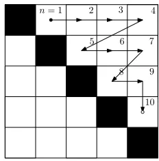
n= 1 2 3 4
5 6 7
8 9
[image:2.612.378.494.48.165.2]10
Fig. 1. Cyclic-by-row execution of Givens rotations implementing one Jacobi sweep, exemplified for a5×5matrix with start sand end point ❝.
algorithm [22]. The term CbR refers to the ordering of the rotations in a sequence like that of Fig. 1, referred to as a Jacobi sweep. While in a standard EVD these are repeated until e.g. off-diagonal elements are suppressed below a given threshold, SMDCbR employs only one Jacobi sweep at each iteration. This equates to a fixed number ofP =M(M−1)/2
Givens rotations for a matrix of size M ×M to provide the unitaryQ(i) in (5),
Q(i)=Q(i,P)Q(i,P−1)· · ·Q(i,2)Q(i,1)= P Y
n=1
Q(i,n). (9)
The iterative process continues forIsteps, say, untilS(I)(z)
is sufficiently diagonalised with the dominant off-diagonal column norm
max k,τ kˆs
(I)
k [τ]k2≤ρ , (10)
below an arbitrarily small threshold ρ. This completes the SMDCbR algorithm and generates an approximate PEVD given by
S(I)(z) =H(I)(z)R(z) ˜H(I)(z), (11)
with
H(I)(z) =
I Y
i=0
U(i)(z) (12)
based on the product defined in (9).
B. Algorithm Complexity
The search step of the SMDCbR algorithm described by (6) uses the column norms of the off-diagonal elements for all lags of the coefficient matrix S(i−1)[τ] ∈ CM×M. If at the
ith iteration S(i−1)[τ] =0∀ |τ| > N(i−1), the search space encompassesM L(i−1)elements, whereL(i−1)= (2N(i−1)+
1) is the length of the parahermitian matrix.
For each sparse rotation during iterationi of SMDCbR, of which there areM(M−1)/2, every matrix-valued coefficient in S(i)′(z) must be left- and right-multiplied with a sparse
Every matrix-valued coefficient in H(i)′(z) must also be
left-multiplied with a sparse unitary matrix for each rotation. A total of2L(Hi)M2(M−1)MACs arise to generateH
(i)(z)
from H(i)′(z), whereLH(i) is the length ofH(i)′(z).
The total number of MACs dedicated towards the rotation step of the algorithm at each iteration is therefore given by
4L(i)M2(M −1) + 2L(i)
HM2(M −1).
III. COMPLEXITY ANDSEARCHSPACEREDUCTION IN
SMDCBR
To reduce the complexity of the SMDCbR algorithm, Sec. III-A and Sec. III-B outline modification to the rota-tion step of the algorithm to concatenate and threshold the Jacobi rotations, respectively. Sec. III-C then details the steps to decrease complexity further by shrinking the algorithm’s available search space at any given iteration.
A. Reduction in Cost of Jacobi Rotations
In the approach detailed here, Givens rotations are per-formed on the zero-lag only, before a concatenated unitary matrix is applied to the entire parahermitian and paraunitary matrices. This unitary matrix is equal to the product of all the sparse rotation matrices applied to the zero-lag. The direct application of sparse rotations to the entire polynomial matrices is therefore avoided, which results in a reduction in complexity.
For each of the M(M−1)/2 sparse rotations, the zero-lag and unitary matrix must be updated. Updating the zero-lag for each rotation involves left- and right-multiplication with a sparse unitary matrix, costing 8M MACs; thus, a full sweep requires 4M2(M −1) MACs. Left-multiplying the unitary matrix for each rotation requires 4M MACs, therefore a full sweep encompasses2M2(M−1)MACs. Both steps combined therefore require6M2(M −1)MACs.
At each iteration, every matrix-valued coefficient inS(i)′(z)
must be left- and right-multiplied with a non-sparse unitary matrix. Accounting for the multiplication of 2M×Mmatrices by M3 MACs, a total of 2L(i)M3 MACs arise to generate
S(i)(z)from S(i)′(z).
In addition, every matrix-valued coefficient inH(i)′(z)must
be left-multiplied with a non-sparse unitary matrix at each iteration. A total of L(Hi)M3 MACs arise to generateH
(i)
(z)
from H(i)′(z).
The total number of MACs dedicated to the rotation stage per iteration is therefore 2L(i)M3 +L(i)
HM3 + 6M2(M − 1) ≈ (2L(i) + L(i)
H + 6)M3 ≈ 2L(
i)M3 + L(i)
HM3 if max{L(i), L(i)
H} ≫ 6. This is approximately equal to half of
the MACs required for the standard SMDCbR algorithm.
B. Thresholding of Jacobi Rotations
As the zero-lag matrix is approximately diagonalised at each iteration of SMDCbR, the off-diagonal elements of S(i)′[0] eventually only contain significant values from the shifted dominant row and column found via (6), with the remaining elements being approximately zero. As these elements possess
very small values, there is little merit in applying a Givens rotation to transfer their energy onto the diagonal.
By incorporating a threshold ν during execution of the cyclic-by-row Jacobi algorithm in SMDCbR, elements with absolute value that fall below this threshold can be ignored.
It should be noted that ignoring Givens rotations in this way reduces the accuracy of the algorithm; however, if ν is kept sufficiently low, this approach can reduce computation time with only a minor impact on algorithm accuracy. Furthermore, the approach described in Sec. III-A does not benefit as significantly as the original SMDCbR algorithm would when employing a threshold for Givens rotations, as savings in the former would only be made during the zero-lag update step; that is, only 12M MACs would be avoided for each missed rotation. The latter would instead experience significant complexity reduction, as each skipped Givens rotation would equate to the avoidance of8M L(i)+ 4M L(i)
H MACs.
C. Limited Search Strategy
Based on previous work [20], [23] to reduce the parameter search space in (6), a further cost reduction for the pro-posed SMDCbR versions is possible by limiting the search of maximum off-diagonal columns to a particular range of lags surrounding lag-zero. The size of this search segment can be determined by estimating the energy distribution in the parahermitian matrix in current or previous executions of the algorithm; using the latter approach can be useful when the data input to the algorithm remains statistically similar between multiple executions of SMDCbR.
A narrow distribution of energy around the zero-lag can therefore lead to a large decrease in search space, and vice-versa. As the algorithm progresses, the lags closest to the zero-lag become increasingly diagonalised, therefore the average delay applied at each iteration increases; this can be accounted for by gradually widening the search space around the zero-lag as the number of iterations increases.
The search step at each iteration of the modified SMD-CbR algorithm described by (6) uses the column norms of the off-diagonal elements for a reduced set of the lags of the coefficient matrix S(i−1)[τ] ∈ CM×M. At the ith
iteration, the search step is applied to a secondary matrix
F(i−1)[τ] = 0∀ |τ| > δ(i−1), which is generated using the L′ = (2δ(i−1)+ 1)centre lags ofS(i−1)[τ]; thus, the search space encompasses onlyM L′elements. If this reduced search space can adequately contain most of the energy from the original parahermitian matrix, then searching for a maximum within this search space can reduce computation time with little impact on algorithm performance. To accommodate the widening of the search space as the algorithm progresses,δ(i) can be described as an increasing linear function ofi.
IV. RESULTS
simula-tion scenario, over which an ensemble of simulasimula-tions will be performed.
A. Performance Metric
Since SMDCbR iteratively minimises off-diagonal energy, a suitable normalised metric defined in [12] is
E(i) norm=
P τ
PM k=1kˆs
(i)
k [τ]k
2 2
P
τkR[τ]k2F
, (13)
with ˆs(ki)[τ] as defined in (7). The metric Enorm(i) divides the off-diagonal energy at the ith iteration by the total energy, which remains unaltered under paraunitary operations; there-fore the normalisation is performed using R(z), which is
only calculated once. For a logarithmic metric, the notation
5 log10E (i)
norm reflects that quadratic covariance terms are squared once more for the norm calculations in (13).
B. Simulation Scenario
The simulations below have been performed over an ensem-ble of 103 instantiations of R(z)∈ CM×M
, M = 5, based on the randomised source model in [12]. This source model generates R(z) = ˜U(z)D(z)U(z), whereby the diagonal D(z)∈CM×M contains the power spectral densities (PSDs)
ofM independent sources. These sources are spectrally shaped by innovation filters such thatD(z)has an order of 120, with a
restriction on the placement of zeros to limit the dynamic range of the PSDs to about 30dB. Random paraunitary matrices
U(z) ∈ CM×M of order 60 perform a convolutive mixing of these sources, such that R(z) has a full polynomial rank
and an order of 240.
The SMDCbR is below referred to as the standard, com-pared to the following four proposed variations:
• method 1: SMDCbR with thresholding of Givens rotations;
• method 2: SMDCbR with concatenation of Givens
rotations;
• method 3: SMDCbR with concatenation and
thresholding of Givens rotations;
• method 4: as in method 3 but with limiting of search space.
During iterations, a truncation parameter ofµ= 10−6and a stopping threshold of ρ= 10−6 were used. The standard and proposed SMDCbR implementations are run over I = 200
iterations, and at every iteration step the metric defined in Sec. IV-A is recorded together with the elapsed execution time.
C. Diagonalisation
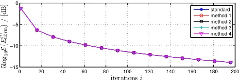
The ensemble-averaged diagonalisation according to (13) was calculated for the standard and proposed implementations. The algorithms incorporating a threshold of ν = 10−3 during diagonalisation (methods 1, 3, and 4) are functionally different to those without this step, but very similar diagonal-isation performance over algorithm iterations can be seen in Fig. 2. The diagonalisation versus algorithm execution time for all methods is shown in Fig. 3. The curves demonstrate
0 20 40 60 80 100 120 140 160 180 200
−15 −10 −5 0
iterationsi
5l
og
1
0
E
{
E
(
i
)
n
o
rm
}
/
[d
B
]
[image:4.612.315.561.53.136.2]standard method 1 method 2 method 3 method 4
Fig. 2. Diagonalisation metric vs. algorithm iterations for the proposed and standard implementations forM= 5.
0 0.05 0.1 0.15 0.2 0.25 0.3 0.35 0.4
−15 −10 −5 0
execution timet/[s]
5l
og
1
0
E
{
E
(
i
)
n
o
rm
}
/
[d
B
]
[image:4.612.316.561.179.263.2]standard method 1 method 2 method 3 method 4
Fig. 3. Diagonalisation metric vs. algorithm execution time for the proposed and standard implementations forM= 5.
that for M = 5, the lower complexity associated with the reduced implementations translates to a faster diagonalisation than observed for the standard realisation.
Thresholding of the Givens rotations in method 1 has a sig-nificant impact on the performance of the algorithm versus the standard algorithm; however, thresholding the same rotations in method 3 does not have such a high impact versus method 2. This is as a result of the thresholding in method 1 eliminating sparse rotations which would have been applied to all lags, while the thresholding in method 3 only eliminates sparse rotations from the zero-lag update step. Despite the small relative impact of thresholding in method 3, this algorithm performs marginally better than all algorithms with a full search space.
Fig. 4 demonstrates that the method 3 becomes more effective relative to method 1 as the spatial dimension M increases, for various values of thresholdν. It can be seen that the benefits of the proposed rotation concatenation approach exceed what could be expected from the calculated complexity reduction, owing to the well-suited nature of the utilised Matlab software for matrix multiplication. Increasing the value ofν decreases the accuracy of both methods, but also reduces the total execution time of method 1 such that it approaches the execution time of method 3. It should be noted that using a threshold of ν = 0 in method 1 is equivalent to using the standard SMDCbR algorithm.
2 4 6 8 10 12 14 16 1
2 3 4 5 6 7 8 9
spatial dimensionM tmet
h
o
d
1
/tm
et
h
o
d
2 ν= 0
ν= 0.0001
ν= 0.001
[image:5.612.53.299.55.163.2]ν= 0.01
Fig. 4. Ratio of method 1 to method 4 total execution time for different spatial dimensionM.
20 40 60 80 100 120 140 160 180 200
0 50 100 150 200 250 300
iterationsi
Lag Number
|τ(i)|method 3 |τ(i)|method 4
L(i)method 3 L(i)method 4
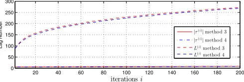
Fig. 5. Parahermitian matrix lengthL(i) and absolute applied delay |τ(i)|
versus iteration number for methods 3 and 4.
search space in the proposed method has been reduced to approximate the 95% confidence interval of absolute delays applied in method 3 in a previous ensemble of103, following the assumption that these values were normally distributed. Using this information, the search space reduction parameter evolution was identified as δ(i)= 0.15i+ 24.
D. Impact on Order of Parahermitian Matrix
The impact of search space reduction on algorithm operation was investigated for method 4, which was shown to perform the best in Sec. IV-C. Fig. 5 shows the ensemble average abso-lute delay|τ(i)|applied to a column in iterationiof methods 3 and 4, alongside the lengthL(i)of the parahermitian matrix in both algorithms. From this figure, it is clear that the reduction in search space does not significantly impact the average delay applied — and thus the order of the parahermitian matrix — at each iteration of the proposed algorithm.
V. CONCLUSION
In this paper, we have proposed a series of steps to reduce the complexity of an existing cyclic-by-row SMD algorithm. We have shown through simulation that this reduction in com-plexity translates to an increase in diagonalisation speed of the algorithm with minimal impact on its accuracy. Furthermore, it has also been demonstrated that a reduction in the search space does not significantly impact the rate of growth of the parahermitian matrix.
When designing PEVD implementations for real applica-tions, the potential for the proposed techniques to reduce com-plexity and memory requirements offers benefits. In addition, the complexity reductions proposed here can be extended to any cyclic-by-row PEVD algorithm by adapting the search and rotation operations accordingly.
ACKNOWLEDGEMENT
Fraser Coutts is the recipient of a Caledonian Scholarship; we would like to thank the Carnegie Trust for their support.
REFERENCES
[1] Z. Wang, J. G. McWhirter, and S. Weiss. Multichannel spectral factor-ization algorithm using polynomial matrix eigenvalue decomposition. In Asilomar SSC, Pacific Grove, CA, Nov. 2015.
[2] C. H. Ta and S. Weiss. A design of precoding and equalisation for broadband MIMO systems. In Asilomar SSC, pp. 1616–1620, Pacific Grove, CA, Nov. 2007.
[3] P. P. Vaidyanathan. Multirate Systems and Filter Banks. Prentice Hall, Englewood Cliffs, 1993.
[4] M. Alrmah, S. Weiss, and S. Lambotharan. An extension of the MUSIC algorithm to broadband scenarios using polynomial eigenvalue decom-position. InEUSIPCO, pp. 629–633, Barcelona, Spain, Aug. 2011. [5] S. Weiss, S. Bendoukha, A. Alzin, F. Coutts, I. Proudler, and J.
Cham-bers. MVDR broadband beamforming using polynomial matrix tech-niques. InEUSIPCO, pp. 839–843, Nice, France, Sep. 2015. [6] S. Redif, J. McWhirter, and S. Weiss. Design of FIR paraunitary filter
banks for subband coding using a polynomial eigenvalue decomposition. IEEE Trans. SP, 59(11):5253–5264, Nov. 2011.
[7] S. Weiss, S. Redif, T. Cooper, C. Liu, P. D. Baxter, and J. G. McWhirter. Paraunitary Oversampled Filter Bank Design for Channel Coding. EURASIP J. Applied SP, 2006.
[8] I. Gohberg, P. Lancaster, and L. Rodman.Matrix Polynomials. Academic Press, New York, 1982.
[9] J. G. McWhirter, P. D. Baxter, T. Cooper, S. Redif, and J. Foster. An EVD Algorithm for Para-Hermitian Polynomial Matrices. IEEE Trans. SP, 55(5):2158–2169, May 2007.
[10] P. Vaidyanathan. Theory of optimal orthonormal subband coders.IEEE Trans. SP, 46(6):1528–1543, June 1998.
[11] S. Icart and P. Comon. Some properties of Laurent polynomial matrices. InIMA Maths in Signal Proc., Birmingham, UK, Dec. 2012. [12] S. Redif, S. Weiss, and J. McWhirter. Sequential matrix diagonalization
algorithms for polynomial EVD of parahermitian matrices. IEEE Trans. SP, 63(1):81–89, Jan. 2015.
[13] J. Corr, K. Thompson, S. Weiss, J. McWhirter, and I. Proudler. Cyclic-by-row approximation of iterative polynomial EVD algorithms. InSSPD, pp. 1–5, Edinburgh, Scotland, Sep. 2014.
[14] J. Corr, K. Thompson, S. Weiss, J. McWhirter, S. Redif, and I. Proudler. Multiple shift maximum element sequential matrix diagonalisation for parahermitian matrices. In IEEE SSP, pp. 312–315, Gold Coast, Australia, June 2014.
[15] J. Corr, K. Thompson, S. Weiss, J. G. McWhirter, and I. K. Proudler. Causality-Constrained multiple shift sequential matrix diagonalisation for parahermitian matrices. In EUSIPCO, pp. 1277–1281, Lisbon, Portugal, Sep. 2014.
[16] Z. Wang, J. G. McWhirter, J. Corr, and S. Weiss. Multiple shift second order sequential best rotation algorithm for polynomial matrix EVD. In EUSIPCO, pp. 844–848, Nice, France, Sep. 2015.
[17] J. Corr, K. Thompson, S. Weiss, I. Proudler, and J. McWhirter. Row-shift corrected truncation of paraunitary matrices for PEVD algorithms. InEUSIPCO, pp. 849–853, Nice, France, Aug. 2015.
[18] J. Foster, J. G. McWhirter, and J. Chambers. Limiting the order of polynomial matrices within the SBR2 algorithm. InIMA Maths in Signal Proc., Cirencester, UK, Dec. 2006.
[19] C. H. Ta and S. Weiss. Shortening the order of paraunitary matrices in SBR2 algorithm. In 6th International Conference on Information, Communications & Signal Processing, pages 1–5, Singapore, Dec. 2007. [20] J. Corr, K. Thompson, S. Weiss, I. Proudler, and J. McWhirter. Shortening of paraunitary matrices obtained by polynomial eigenvalue decomposition algorithms. InSSPD, Edinburgh, Scotland, Sep. 2015. [21] F. Coutts, J. Corr, J. Thompson, S. Weiss, J. Proudler, and J. McWhirter.
Memory and complexity reduction in parahermitian matrix manipula-tions of pevd algorithms. Submitted toEUSIPCO, Budapest, Hungary, August 2016.
[22] G. H. Golub and C. F. Van Loan.Matrix Computations. John Hopkins University Press, Baltimore, Maryland, 3rd ed., 1996.
[image:5.612.53.298.204.287.2]