City, University of London Institutional Repository
Citation
:
Jafarey, S. and Maiti, D. (2015). Glass slippers and glass ceilings: An analysis of marital anticipation and female education. Journal of Development Economics, 115, doi: 10.1016/j.jdeveco.2014.12.005This is the accepted version of the paper.
This version of the publication may differ from the final published
version.
Permanent repository link:
http://openaccess.city.ac.uk/6565/Link to published version
:
http://dx.doi.org/10.1016/j.jdeveco.2014.12.005Copyright and reuse:
City Research Online aims to make research
outputs of City, University of London available to a wider audience.
Copyright and Moral Rights remain with the author(s) and/or copyright
holders. URLs from City Research Online may be freely distributed and
linked to.
City Research Online: http://openaccess.city.ac.uk/ publications@city.ac.uk
Glass slippers and glass ceilings: An analysis of
marital anticipation and female education.
Saqib Jafarey*
Dibyendu Maiti
†January 9, 2015
abstract
This paper studies how marital anticipation affects female schooling in the presence of gender wage inequality and private benefits of education. Gender wage inequality induces a marital division of labor that creates (i) a marginal disincentive to girls’ schooling and (ii) a tradeoff between consumption and education facing females in marriage markets. We show that in the presence of the last effect, an increase in the market wage can have negative consequences for the education of females who specialise in housework.
Keywords: Female education, labor market discrimination, marriage. JEL Classification: I20, J12, J16, O12.
Acknowledgements: We thank Ravi Mukherjee for discussions which led to this paper and Michael Ben-Gad, Gabriel Montes-Rojas, Maria Iosifidi, Javier Ortega, Bishnupriya Gupta and Sajal Lahiri for helpful comments. Two anonymous referees and an editor have made very insightful comments and criticisms which we believe have greatly strengthened our arguments. All remaining errors are our own.
*Jafarey (corresponding author): Department of Economics, City University, Northamp-ton Square, London EC1V 0HB, United Kingdom and School of Economics, University of the South Pacific, Suva, Fiji. E-mail for correspondence: s.s.jafarey@city.ac.uk.
† Maiti: Institute for Economic Growth, University of Delhi Enclave, New Delhi, India
1
Introduction.
Females in developing countries have traditionally received less education than males.1
There is also evidence of anti-female bias in child nutrition and healthcare (see, e.g.
Khanna et. al. [2003]). A common economic explanation is that these biases
rep-resent optimal parental responses to gender inequalities in returns to labour and
human capital (see Rosenzweig and Schultz [1984] for a seminal investigation of this
hypothesis). Faced with lower returns to females, parents shift resources towards
males.2
Gender biases in survival tend to get eliminated as household incomes rise above
poverty (Deaton [1989] and Rose [1999]). For biases in education, cross- and
single-country studies using aggregate data suggest that these too might gradually disappear
with increases in per-capita incomes. For example, in a comprehensive cross-country
study, Mammen and Paxson [2000] find that average years of female schooling rise
monotonically with per-capita income.
However, aggregate data can mask composition effects across different income strata
within a country. For example, in low and lower-middle income countries, where a
significant proportion of females receive either no or sub-primary levels of education,
gains at low levels of achievement would lead to an increase in average years, even
if there is stagnation at higher levels.3 Indeed, even Mammen and Paxson’s fitted
1See Dreze and Kingdon [2000], Grootaert [1998], Ilahi [1999], Ilahi and Sedlacek [2000], Ray
[2000]. As an exception, Munshi and Rosenzweig [2004] find that among lower-caste Marathas, girls are more likely than boys to receive a modern English education, as opposed to a traditional Marathi one. The arguments of this paper are broadly consistent with both types of findings.
2In this paper, we shall assume that there is gender wage inequality, while noting that the
empirical evidence for this claim is mixed. Kingdon [1998] and Nasir [2002] found evidence for lower returns to girls’ schooling in India and Pakistan respectively, whereas Behrman and Deolalikar [1995] and Aslam [2009] found the opposite to be true in, respectively, Indonesia and Pakistan.
3In South Asia, among the age group of 15 years and more, Afghan females have an average of
regression lines suggest that the marginal impact of per-capita income declines at
low combinations of per-capita income and educational achievement – until roughly
1000 USD of income and 2 years of schooling – and only begins to show a steady
increase after this threshold has passed. Moreover, they also show that over roughly
this same interval, the educational gender gap widens.
In a paper that analysed the impact of economic growth on gender inequality across
different levels of education, Dollar and Gatti [1999] found that while economic growth
generally reduced gender inequality, in the ‘important’ area of secondary education,
females tended to lag behind males until a threshold level of per-capita income of
about 2000 USD had been passed.4
Gender gaps in enrolment are listed by level of education for a selection of low and
lower middle income countries belonging to Africa, South Asia and Southeast Asia
respectively. The first sub-column under level of schooling pertains to levels and the
second sub-column to the average annual rate of increase in gender parity since 1999.5
years) and “only” 35% of females receive no education (Barro and Lee [2011]).
4Dollar and Gatti [1999] also split their sample in half on the basis of PPP-adjusted per-capita
income. They found that there was no statistical relationship between female enrolment and per-capita income, controlling for other factors, for the poorer sub-sample but a significant positive one for the richer one.
5Average rates of change in gender parity were taken to smooth out the year-to-year noise,
Female:Male Enrolment Ratio, 2011
Primary Secondary Tertiary
Average Average Average Country Level Annual Level Annual Level Annual Growtha Growtha Growtha
Burkina Faso 93 2.33 78 2.11 50 2.83 Guinea 87 2.27 64 4.4 36 8.4 Ghana 100 0.65 91 0.98 62 3.55 Afghanistan 71 5.97 55 8.605 23 N/A Bangladesh N/A N/A 117 1.33 70 2.26 Indiab 100 2.25 92 2.48 73 1.53 Pakistan 82 1.88 73 -0.65 91 0.75 Cambodia 95 0.72 85c 5.07 61 6.04 Indonesia 102 0.49 100 0.47 87 -0.013 Lao PDR 74 3.75 94 0.83 86 1.72
Source:World Development Indicators: http://data.worldbank.org/data-catalog/world-development-indicators;a: Percentage rate of change in gender parity, averaged from available data over the period 1999-2011;b: all data from 2010;c: secondary school data from 2008;
One feature of the data is that, Pakistan and Lao PDR excluded, disparity increases
with level of education. Second, apart from countries that already had high gender
parity in primary enrolment by 1999-2000 (Cambodia = 87%, Ghana = 93% and
Indonesia = 97%) the other countries have shown increases at the average rate of
1.9%-3.8% per annum in this ratio. This suggests that primary education is more
or less moving towards equality albeit the Muslim South Asian countries of Pakistan
and Afghanistan are lagging.
In the case of secondary and tertiary enrolment, there appears to be a wider dispersion
in both levels and trends. Pakistan and Indonesia have the highest parity ratio in
tertiary education but the data for both show significant ups and downs in this ratio,
resulting in trends that are either low or negative.6 Also note that the countries
that had the lowest gender parity in higher education at the end of the millennium
(Cambodia = 32% in 2000, Burkina Faso = 30% in 1999, Guinea = 19% in 2003)
showed the highest growth rate but that is more a matter of having started with low
6In particular, Pakistan’s reported gender gap in tertiary education is quite anomalous in light of
denominators in the growth rate calculation
It is also worth noting that countries that are showing a reversal of the gender gap
in secondary education, Bangladesh and Indonesia, are countries in which concerted
efforts have been made to expand educational opportunities and social protection
programmes over the last couple of decades.7 Even in these countries, however, the
gap between male and female tertiary enrolments remains considerable. All in all,
the above data suggest that with respect to the above selection of low and lower
middle income countries gender disparity in enrolments continues to be significant at
all levels for a few countries, at secondary levels for a larger group and at tertiary
levels for almost all.
Since within a country higher levels of education tend to be the preserve of
progres-sively higher-income households, who also tend to have smaller family sizes, one would
expect gender gaps to be narrower at this level, even if the country itself is a lower
income country in which overall enrolments are low. That it does not, weakens the
hypothesis that gender gaps are due to rationing by income- and credit -constrained
households and implies that there might be other factors that impede the progress
of female education as incomes grow, both cross-sectionally within a country and
inter-temporally as its economy grows.
In this paper, we analyse the effect that the anticipation of marriage has on the gender
gap in schooling. We show that marriage exacerbates labour market inequality by
inducing a household division of labour that encourages females to spend time doing
housework. In our model, formal education has the conventional monotonic, linear
effect on market earnings, but a non-monotonic, inverse U-shaped effect on household
skills. This creates the potential for an anti-female bias in education. We show that
the bias is multiplicative in that marriage can lead to an even stronger anti-education
7However, Haq and Rahman [2008] report that while secondary school enrolments are higher for
effect than if the same female was expected to remain single. It is also discontinuous
in the gender wage gap, i.e. a progressive reduction in wage inequality does not
progressively eliminate the education gap.
We further compare female educational outcomes across two scenarios concerning
marriage formation. In the first, a solitary pair of male and female are exogenously
assigned to marry, with their optimising decisions on education and labour supply
following from this inevitability. In this case, each of them receives a share of
ri-valrous household resources that is also set exogenously. In the second scenario,
marriage formation requires the couple’s mutual consent. In this case, the division of
rivalrous resources becomes an important component of the decision to marry, and is
endogenously determined via pre-nuptial negotiation between the couple.
We refer to the first scenario as exogenous marriage formation and the second
inter-changeably as consensual marriage formation or in brief consensual marriage.8,9
In the context of consensual marriage, we show that each partner’s share of rivalrous
resources depends on their respective bargaining power and that this dependence can
create additional constraints on female education. The crucial assumption here is
that agents derive a degree of private utility from education, in addition to its human
capital-enhancing benefits and any contribution it makes to marital companionship.
Under exogenous marriage formation a female’s optimal education level is determined
8The term ‘exogenous marriage’ has been used by some authors to refer to what is more precisely
known as ‘exogamy’: marriage outside one’s own kinship group (see,e.g., Herlihy [1995]); to avoid confusion we use ‘exogenous’ to condition the term ‘marriage formation’, which has been used by other authors, e.g., de Moor and van Zandan [2010], to refer to the mechanism through which couples are assigned to marriage. To our knowledge no semantic confusion arises between the terms ‘consensual marriage formation’ and ‘consensual marriage’ so these will be used interchangeably.
9The term ‘consensual’ has been used by de Moor and van Zandan [2010] in describing what
without taking into account the effect it will have on her spouse’s utility. Under
consensual marriage creation, by contrast, both partners will take into account how
the other’s welfare is affected by their own choices. Take the case where marriage
leads the female to specialise in housework. From the male’s point of view, her
optimum education will be the one that maximises her housework skills but the
female herself would prefer a higher level, depending on the strength of her private
taste for education. In anticipation of pre-marital bargaining, the female’s parents
could restrict her education in order to make her more attractive to her partner and
strengthen her bargaining power over the rivalrous resources created by their union.
We also show that if the market wage goes up, with no change in the degree of
discrimination, her level of education might fall. This is because an increase in the
market wage can, under plausible circumstances, increase the value of the male’s
outside option more than it does the female’s. Of course, if the wage is high enough
so that a married female supplies positive labour, the need to contribute through
housekeeping skills becomes less important and her education can respond positively
to further increases in the market wage.
The restrictive impact of consensual marriage on female education need not apply
to all levels of schooling. Rather we assume that up to a point, exposure to
for-mal schooling complements hands-on experience in the acquisition of domestic skills.
There is an optimal combination of the two at which domestic skills are maximised.
It is only after this level has been passed that a conflict will arise between a female’s
education and her domestic skills. The potential for such a conflict is greater at high
levels of schooling than at low ones.
Lahiri and Self [2007] have also argued for the disincentive effect of marriage on
female education Their argument is based on patrilocal living arrangements that
marriage will contribute to their in-laws’ household, while sons will contribute to
their natal households.10
By contrast, Behrman et. al. [1999] argue that the prospect of marriage can
encour-age female education. This is because women play a role in providing home schooling
to children. Thus more educated women are more desirable on the marriage market
as they are likely to be more effective home teachers. One implication of their model
is that with economic growth, the demand for sons’ education will go up, leading
to an increase in demand for educated brides and mothers, even if their own labour
market participation is low. Using data sets from India, they find evidence in support
of their hypotheses.
Behrman et. al. seem to negate our main argument, especially since our paper
shares important features with theirs: namely, gender wage inequality, specialisation
in household duties and marital selection based on female education. Yet the papers
are not mutually incompatible. For one thing, Behrman et. al. focus on agricultural
settings in which both the level of education needed to enhance farm productivity
and the mother’s own education level are implicitly at the primary level. Our paper
is more applicable to urban middle class settings in which men earn enough to allow
their wives to specialise in home production. In these settings, a primary level of
education is a foregone conclusion for both genders.
Moreover, if we interpret the household production function of our paper as
incor-porating the task of home schooling then Behrman et. al.0s argument implies that
as wages increase, the optimum level of education to maximise household skills also
increases. Indeed, if this effect is strong enough then it can lead to an increase in
female education at even post-primary levels. Having acknowledged that possibility,
10Lahiri and Self [2008] extend this line of argument to explain the anti-female bias in survival
our paper identifies a channel through which a private taste for education
interact-ing with pre-nuptial bargaininteract-ing will, given a fixed technology for the production of
household skills, create a countervailing effect against female education. Which of the
two effects dominates is an empirical matter but the point is that these two channels
are not mutually exclusive.11
Chiappori et. al. [2009] also provide a rationale for the pro-education effect of
marriage. This result follows from the effects of marital sorting on schooling choice
when schooling not only enhances labour market returns but also the share of the
marital surplus accruing to the relevant spouse. While that paper’s analysis of the
sorting process is more detailed than ours, it’s model restrict education to a binary
0-1 choice with no variation across levels of education. The authors also treat the
marital surplus as a black box which increases in the combined education of the
two spouses, without decomposing it into a rivalrous and non-rivalrous goods as we
do. Thus the possibility that the marriage surplus might be non-monotonic in the
combined schooling of the two spouses is not present in their model while in ours, it is
precisely that possibility that creates a tension between a female’s education and her
marriageability and might lead her to lower her educational level in order to enhance
her household skills and increase her bargaining power on the marriage market.
In economic theory, formal education is assumed to enhance marketable human
cap-ital. If one applies this interpretation strictly, education should be measured not just
by years of schooling but by years weighted by a metric of marketable skills which
dif-fers according to subject specialisation. Marital matching might then operate through
the couple’s respective fields of study and not just their years in education. In that
case, less ‘formal’ schooling might mean less exposure to subjects that enhance
mar-11Indeed, even in our given technology for producing household skills, dropping the private desire
ketable human capital and more time studying subjects that enhance domestic skills.
Folbre and Badgett [2003] and Fisman et. al. [2006] have, in separate experiments,
linked gender differences in fields of study and occupational choice with differences
in how males and females rate each other in terms of attractiveness. While the
for-mer authors found that both men and women who reported studying for or holding
non-stereotypical occupations were rated as less attractive by members of the other
gender, the latter found that females are more likely to select male partners on the
basis of higher intelligence and ambition while males are more likely to use physical
attractiveness as a criterion. Moreover men did not value women’s intelligence or
ambition when it appeared to exceed their own. Although the context of our paper
is different from the above two, its arguments shed some light on their findings.
The rest of the paper is organised as follows. Section 2 describes the model. Section
3 analyses the labor market and educational decisions of single individuals. Section
4 analyses the analogous decisions for individuals whose marriage is determined
ex-ogenously. Section 5 analyses the decision to marry in the context of a single male
and single female and Section 6 analyses specific examples and presents numerical
results for the preceding sections. Section 7 considers a marriage market in which
each agent has a choice over partners. Section 8 offers concluding remarks.
2
The model.
There are two households, labelled X and Y respectively. Each has one offspring,
intrinsically identical save for gender: X is male and Y is female. Each offspring
proceeds through two stages of life: childhood and adulthood. In each stage of life
they have a time endowment equal to unity.
child’s time between formal schooling and domestic training. This allocation
deter-mines the combination of labour market versus household skills that the child grows
up with.
2.1
Labour market skills and household skills.
Labelling time spent in schooling as s ∈ [0,1], and the level of human capital as e,
we follow the literature in assuming a linear relationship, e=s.12
Household skills are denoted by α. Unlike market skills, the optimal development
of household skills requires positive inputs of both formal schooling and domestic
hands-on training. At one extreme, a child who spends all his or her time performing
domestic chores might not pick up the basic literacy and numeracy skills needed to
run a household. At the other extreme, a childhood spent entirely in formal schooling
would lead to no direct training in domestic chores.
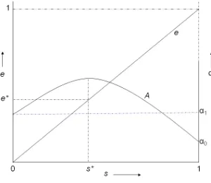
The above properties are captured by a function: α=A(1−s) that satisfies:
(A-1): A(·) is continuously differentiable and strictly concave for all s∈[0,1].
(A-2): A(1−s)≥0 ∀s∈[0,1];A(0) ≡α0;A(1)≡α1.
(A-3): ∃a unique s∗ ∈[0,1) such that A(1−s∗)≡α∗ =max{A(1−s)} ∀s∈[0,1].
Together with (A-1), (A-3)guarantees that household skills are maximised only when
a strictly positive amount of domestic training is undertaken along with formal
edu-cation.
The level of formal education that maximises household skills might increase with
the state of development of the society and the social class to which the household
belongs. At higher levels of development and in higher social strata, not only literacy
Figure 1: Household Skills and Market Skills
and numeracy but also exposure to the arts, history and literature might be important
for the development of domestic skills. What is important is that there is some point
at which further development of market skills comes into conflict with the formation
of household skills.13
Figure 1 illustrates the combinations of household skills and formal education that
result from any given choice of s. The horizontal axis measures time in schooling,
s, which lies between zero and unity. The vertical axis on the left measures formal
education, e, which lies between zero and unity, increasing linearly with s . The
vertical axis on the right measures housekeeping skill, α. Time spent in housework
as a child decreases as s rises. Accordingly, at s = 1, α=α0. At s = 0,α =α1 and
at s=s∗, α= ¯α.
At any value of s, α and e are uniquely related. This relationship may be expressed
as :
α=A(1−e)
13Formally, the results of this paper merely require that household skills are a continuous function
where α=α0 when e= 1, α=α1 when e= 0 and α= ¯α whene =e∗.
In the second period, the adult decides whether to marry or not, moves out
accord-ingly and makes a time-allocation decision between market work (`) and housework
(1− `). This decision is made conditional on the individual’s marital status and
market wage. The latter in turn depends linearly on an underlying wage ωi and the
individual’s human capital ei through the linear function:
wi =ωiei (1)
wherewi represents the hourly wage, andωi is an underlying return to human capital.
Wage inequality implies thatωis not the same for both genders. A parametric manner
to express this is that there is an underlying market wage ω and that ωX =ω while
ωY =φω,φ ≤1.
2.2
Preferences and constraints.
We assume that childhood utility is separable from adult utility and does not depend
on the choice between schooling and household chores. Each adult has a utility
function:
Ui =u(ci) +hi+bei (2)
i=X, Y;u(·) is a concave function of the adult’s consumption of a rivalrous market
good, satisfying u0(0) = ∞; hi is the utility from consumption of a household good.
The last term in the utility function represents a non-pecuniary private benefit that
an adult derives from being educated. The possibility that education confers private
develop-ment literatures but is not without precedent in the broader literature on education.14 These benefits could be direct: education confers pride and satisfaction for its own
sake, or indirect: education enables individuals to seek out information which leads
to better choices.
An example is the link between education and health explored in the health literature.
As summarised in Cutler and Lleras-Muney [2006], a large body of evidence exists
for a positive relationship between health and education, even after accounting for
the effects of education on income. Their argument is that education leads to better
decision-making and information-seeking and thus helps individuals maintain good
health.
This assumption plays an important role in our analysis of female education
through-out the paper but especially in comparing through-outcomes across different types of marital
institution. We shall show that the presence of a private benefit from education leads
to an externality in the case of married agents: each agent values their partner’s
education less than the partner does. The relevance of this externality is related to
the labour market participation of each spouse. For example, if a married male
spe-cialises in market work while a married female spespe-cialises in housework, the male’s
private preference for education will be inconsequential to the female, but not the
other way around. This asymmetry will affect the marital decision-making process
for each prospective spouse.
For a single individual, market consumption is:
ci =wi`iei; i=X, Y; (3)
where ` denotes the fraction of adult time spent in market work.
14See, for example, early attempts to empirically disentangle these two effects by Schaafsma [1976]
If married, the consumption of the market good will be subject to a market budget
constraint:
cX +cY =wX`XeX +wY`YeY. (4)
The utility from consumption of the household good depends on the amount of
ef-fort put into household production according to a concave function. For a single
individual, the utility is given by
hi =h(αi(1−`i)) (5)
where αi is the individual’s level of household skills and (1−`i) is adult time spent
in household production. We assume that h0 >0,h00 <0 and thath0(0) =∞.15
For married households, we assume that there is (i) a single production function per
household; (ii) the ability-adjusted effort levels of each spouse are mutual perfect
substitutes and (iii) the household good is a pure public good.16
hX =hY =h(αX(1−`X) +αY(1−`Y)) (6)
2.3
Decision making.
We first impose the state of being married or remaining single and within each state
we solve for the agents’ time allocations, taking as given their levels of schooling;
then in solving for the latter we take into account its effect on adult time allocation.
We assume that regardless of whether their union is formed exogenously or
consen-sually, couples decide on their respective time allocation in a unitary fashion. This
15The concavity of h(·) can be interpreted in two ways: either that the household production technology is itself concave or that the utility of household goods is concave, or both.
16In another paper, Jafarey [2008], the assumption that the household good is a pure public good
assumption is made partly to elaborate on Becker’s [1973] approach by exploring
the role of wage inequality in creating the mutual comparative advantage that each
partner brings to marriage, which then leads to a household division of labour on the
basis of efficient time-use by each partner. It is also made partly because assuming
non-cooperative decisions on time use could by itself lead to some of the asymmetries
in outcomes that characterise our results. Basu [2006] has already shown that with
non-unitary decision-making, the allocation of household resources depends crucially
on each members contribution to household income. In addition, Rainer [2008] has
shown that under conditions of wage discrimination, intra-household bargaining leads
to a magnification of gender inequalities in time allocation. In that sense, the results
of this paper show that such a magnification effect can arise even when the time
allocation of each spouse is jointly welfare-maximising. Furthermore, Behrman et.
al. [1999] show that when education increases spousal bargaining power, prospective
husbands become biased against female education for that reason. Our arguments
pursue a different channel for such effects so assuming unitary decision-making ties
our hands against the predicted outcome.
Moving back from the time allocation decision, we consider the marital decision,
com-paring outcomes under exogenous marriage formation with those under consensual
formation. We have already noted the importance of side payments in the latter case.
Since there are no bequests or outside assets in our model through which transfers
such as dowries could be financed, the share of each partner’s consumption in the
rivalrous market good becomes the main source of side payments. We assume that
a enforceable contract can be written over these shares through a pre-nuptial
agree-ment between the spouses. We also assume that the exact division is the one that
equalises the gains from marriage relative to an appropriate outside option for each
spouse. We initially assume that each prospective spouse’s only outside option is to
extend this to a setup in which each partner faces a rival in the marriage market.
In the last step of our analysis, the education decision itself is analysed. In principle
this should take into account the impact of each child’s education on his or her future
time use in each state of adulthood, along with its effect on his or her post-nuptial
share in consumption in case of consensual marriage. In practice, this is done in all
states only for a female; for a male we impose a corner solution on both labour supply
and education in all but the state of remaining single.
In discussing the various cases, we shall refer to the “single self” of a married agent
as the same agent had he or she not got married and likewise, the “married self” of
a single agent as that agent had he or she got married.
3
Single agents.
On reaching adulthood, the agent’s human capital e has been fixed, as has α (agent
subscripts are suppressed since the problem is qualitatively identical for both). The
agent maximises utility with respect to labor market participation, `.
Plugging the adult budget constraints into the utility function, the maximisation
problem is expressed as:
max
`
=u(ωe`) +h(A(e)(1−`)) +be
which has first-order condition:
u0(·)ωe−A(e)h0(·) = 0 (7)
speciali-sation is ruled out by Inada conditions.
The interpretation is analogous to the one in the standard case of endogenous labor
supply when leisure counts for its own sake. Here, the trade-off becomes one between
market and home labor. A small increase in market labor increases utility from the
market good by u0(·)ωe but reduces that from the home good by h0(·)α. At the
optimum, the two effects cancel out.
The resulting solution can be expressed as`(ω, e). As is well known, a non-monotonic
relationship between labor supply and the market wage is possible. A necessary and
sufficient condition to rule this out is:
(A-4): u0(c) +u00(c)·c > 0
Under (A-4) it can be established that `ω > 0 (see Lemma 3, Appendix). Since
changes in e can also affect equation (7) through the home production function,
(A-4) is by itself not sufficient to rule out `e ≤ 0 but imposing a further sufficient
condition ensures that `e >0:
(A-5): h0(α(1−`)) +h00(α(1−`))α(1−`)>0
(A-4) and (A-5) are in line with conventional restrictions imposed to prevent
‘back-ward bending’ labor supply and allow us to set benchmarks for comparing time
allocation across genders and marital states.
The decision on education is taken by a parent during childhood.17 We assume the
parent takes into account the implications of education on adult outcomes. The
problem can be expressed as:
max
e
=u(ωe`(e)) +h(A(e)(1−`(e))) +be
17This is mainly for expositional purposes. We could equally have the child taking it themselves,
The first-order condition is:
u0(·)ω`+b+h0(·)(1−`)A0(e)≥0 (8)
The first-order condition can only be satisfied at e≥eˆ. But there is no incentive to
choosee <ˆesince ˆeis the amount of education where household skillα is maximised.
If the first-order condition is satisfied with equality, e≤ 1. If, as a strict inequality,
e = 1. The intuition is that a small increase in education will increase the utility
from consumption, at given wages and market labor supply by an amount u0(·)ω`
and the private utility from education by b, while the utility from home production
will fall, at given levels of home work and production, due to a fall in home skills α
by an amount A0(e). These effects cancel out at the optimum.
Proposition 1 below establishes the effect of wage inequality between otherwise
iden-tical agents
Proposition 1: Suppose that (A-4) and (A-5) hold, then an increase in the wage, ω
will, for given underlying characteristics, lead to higher education eand more labour
supply `.
Proof: See Appendix.
The intuition behind Proposition 1 is that a higher wage tilts the first-order condition
with respect to education towards acquiring more market skills and less household
skills. For given education, it also tilts the balance in favour of supplying more
market labour (due to (A-4)) and less household work. Under (A-5) the latter will
be reinforced by the increase in education. Thus on the whole, market labour will also
go up. Applied to gender wage inequality, Proposition 1 implies that a single male
will acquire more education and supply more labour than an intrinsically identical
the single male and the single female, as the wage gap narrows so will the gap in
outcomes, until a benchmark of wage equality and symmetric outcomes is reached.
Form hereon, whenever the context does not by itself make clear whether we are
referring to the cases of single agents, exogenously formed marriages or consensually
formed ones, superscripts will be used to distinguish them: single selves’ outcomes
are labeled es
i and `si; while married selves’ outcomes are labeled as either eai and `ai,
or em
i and `mi , i =X, Y, depending on whether marriage formation is exogenous (a)
or mutually consensual (m).
4
Exogenous marriage formation.
As explained before, we assume unitary decision-making in regards to the time use
of married adults. The household utility function can be expressed as:
V ={u(cX) +hX +beX}+{u(cY) +hY +beY}
Only the first four terms of the utility function are affected by the choice of labor
market participation. Given the exogenous nature of marriage in this section, we
further assume for the sake of saving on notation that the market good is shared
equally: cX =cY.18
The time allocation problem now reduces to:
max
{`X, `Y}
V = 2u
ωeX`X +φωeY`Y
2
+ 2h(A(eX)(1−`X) +A(eY)(1−`Y))
18This allocation would result from unitary household decision-making, given symmetric utility
which has first-order conditions:
u0(·)ωiei−2A(ei)h0(·)≥0;
which is more usefully rearranged as:
ωiei
A(ei)
≥ 2h
0(·)
u0(·) ; (9)
i=X, Y.
In choosing education, we assume that the parents care only for the welfare of their
own offspring. We also assume that parents take into account the effect of their
own child’s education on own adult labor supply but not the spouse’s. Each parent
maximises the following function:
max
{ei}
u
ωiei`i(ei) +ωjej`j
2
+h(A(ei)(1−`i(ei)) +A(ej)(1−`j))+bei; i, j = (X, Y)
The first-order condition is (terms involving the effect ofeon adult labor supply drop
out when evaluated at the optimum):
0.5u0(·)ωi`i+h0(·)(1−`i)A0(ei) +b ≥0; (10)
i = X, Y. It is clear from equation (9) that when φ < 1, both spouse’s first-order
conditions cannot simultaneously hold as equalities. This means that an interior
solution for labour supply cannot simultaneously hold for both spouses: either one
will specialise in market work, or the other in housework or both. Which spouse does
what can be determined by considering the implied inequalities in (9). Suppose that
when φ <1, ωXeX/A(eX)≥ωYeY/A(eY). In that case. three possible combinations
housework at the level of the household):
(i) ωXeX
A(eX) >
ωYeY
A(eY) = 2h0(·)
u0(·);
(ii) ωXeX
A(eX) > 2h0(·)
u0(·) > ωYeY
A(eY);
(iii) ωXeX
A(eX) = 2h0(·)
u0(·) > ωYeY
A(eY).
(11)
In case (i) `X = 1 while `Y ≥0; in case (ii) `X = 1 while `Y = 0; in case (iii) `X ≤1
while`Y = 0. Either the male specialises in market work, or the female in housework
or both.
Proposition 2 below in fact establishes that when φ < 1, then eX > eY in turn
implying that ωXeX/A(eX) ≥ ωYeY/A(eY) (since education is always chosen along
the decreasing portion of the household skills curve, A(e)).
Proposition 2: In the presence of wage discrimination (φ < 1) the higher paid spouse chooses an education level at least as high as that chosen by the lower paid
spouse (eX > eY).
Proof: See Appendix.
While Proposition 2 covers all three cases concerning the division of tasks by a married
couple, we shall henceforth neglect case (iii) in favour of the cases of our main interest.
How do the labor market effort and educational levels of the married female compare
with that of her single self?19 Conditioning on a given level of female education, the comparison of her market labour is stated in Proposition 3.
Proposition 3: Given the same level of female education eY in both possible states
regarding marital status, a married female supplies less market labour than a single
19A comparison between the married male and his single self is made in (Jafarey [2008]) where
one.
Proof: See Appendix.
The intuition behind Proposition 3 is that even if the married female were to have
the same level of education as her single self, it would be efficient from the marital
household’s point of view to make use of her spouse’s comparative advantage in
providing market income by allocating her to do more housework than she would as
a single female.
In comparing education choice between married and single females, a straightforward
comparison of equation (8) the first-order condition for a single female’s education,
and equation (10), the analogous condition for a married female, suggests that at
given values ofeY and `Y, the LHS of the former equation exceeds that of the latter.
This is because for a married female, the marginal impact of education on market
income is discounted relative to that of her single self.20 Other terms in the two equations are identical for both selves.21 Thus, at given levels of market participation, a married female will receive less education than her single self. In fact, especially
in light of Proposition 3, we expect that a married female’s education will be further
discounted because of lower market participation than her single self.
This intuition is formalised in Proposition 4.
Proposition 4: When married to a male who specialises in market work, a married female will attain less education and supply less market labour than her single self.
20This is also true for a married male relative to his single self. The difference is that when
a married male specialises in market work, his first-order condition for education will hold as an inequality regardless of the discount.
21Jafarey [2008] considers a setting in which the household good is partly rivalrous. In this case,
Proof: See Appendix.
Proposition 4 notwithstanding, the next section will go on to argue that consensual
marriage might restrict a married woman’s education even more than exogenous
marriage formation.
Finally note that the labor supply of married adults reacts discontinuously to gender
wage discrimination. Equation (11) has established the existence of specialisation in
time use when φ < 1. On the other hand, if there was gender wage equality, i.e.
φ = 1, then the first-order conditions for both spouses would be symmetric and it
can be shown that `X =`Y and eX =eY.22 This shows that due to the possibility of
specialisation, even a small amount of wage discrimination can discontinuously induce
corner solutions in the time use and education levels of one or both married agents.
This is not true for their single selves, since their labor market and education levels
vary continuously and identically with their respective wages . Thus as ωY −→ ωX,
the time allocation and education of single agents converge towards each other.
5
Consensual marriage.
We now endogenise marriage formation while continuing to base our analysis on a
solitary pair of male and female. In Becker’s [1973] analysis, it is implicit that
po-tential partners differ in their respective labour and homemaking characteristics, so
that married couples gain by exploiting these differences on the basis of mutual
com-parative advantage. With gender wage inequality, asymmetry creeps in through
dif-ferences in time allocation and gets reinforced by education choices, even if potential
partners are intrinsically identical. As a result of both the wage and the educational
gap, the male partner may end up with a comparative advantage in market work and
the female in housework.
With consensual marriage, a selection criterion needs to be satisfied for both partners:
Uim ≥Uis i=X, Y.
whereUm stands for the utility from entering into consensual marriage andUs is the
utility from staying single.
We assume that the couple are able to realise any potential gain from marriage by
making a binding pre-nuptial agreement on post-marital outcomes. Since neither has
a direct preference over how to use their time, we assume that they agree to let their
respective duties be determined by a unitary decision-making process. But since they
do care about their own consumption of the market good, they can bargain over their
share of it. Letµdenote agentY0s share of the market good, so that (1−µ) is agent
X0s share.23 In the context of this model, where there are no external assets, bequests
or other means to make side transfers, this is the only form in which such payments
can be made in order to realise the possible gains from marriage. In addition, we
assume that the pre-nuptial bargain results in consumption shares that split the gains
from marriage equally between the two partners. Because of the existence of only one
possible spouse, the outside option for each agent is the maximum utility they could
derive from remaining single. The next section extends this to a set-up in which the
outside option includes a choice of partners.
Given µ, the time allocation of the married couple follows analogously to the case
of exogenous marriage. The difference is that the endogenous consumption share
replaces the exogenously determined 50:50 split that was employed in the case of
exogenous marriage formation. The first order conditions for the optimal time
allo-cation lead to the following analogous cases.
(i) ωXeX
αX
> ωYeY αY
= 2h
0(·)
µu0Y(·) + (1−µ)u0X(·);
(ii) ωXeX
αX
> 2h
0(·)
µu0Y(·) + (1−µ)u0X(·) >
ωYeY
αY
;
(iii) ωXeX
αX
= 2h
0(·)
µu0Y(·) + (1−µ)u0X(·) >
ωYeY
αY
.
Three cases are again possible: in case (i) `X = 1 while `Y ≥ 0; in case (ii) `X = 1
while `Y = 0; in case (iii) `X ≤ 1 while `Y = 0. Since our focus is on those cases in
which a married male specialises in market work and his education is at its maximum
we shall ignore (iii).
In modeling the choice of female education, we now take into account not only its
impact on the time-use decision, but also its effect on her share of the
consump-tion good µ arising from pre-nuptial bargaining. This problem is formally stated as
(superscripts m denote consensually determined marriages):
max
{em Y, µ}
UYm = u(µω(1 +φemY`mY(emY, µ))) +h(A(emY)(1−`mY(emY, µ)))
+bemY (12)
s.t.
UYm−UYs ≤ {u((1−µ)ω(1 +φemY`mY(emY, µ))) +h(A(emY)(1−`mY(emY, µ)))
+b} −UXs (13)
where Uis = u(ωiesi`si) +h(A(esi)(1−`si) +besi; i = {X, Y}. The constraint simply
states that the female’s gain from marriage is no greater than the male’s. Relative
creates the possibility that consensual marriage can, under some circumstances,
fur-ther discourage female education. Noting that the utility from consumption of the
household good enters both sides of the marital selection constraint, the Lagrangean
associated with the above problem can be written as
L =UYm+λh[u((1−µ)ω(1+φemY`mY(emY, µ)))+b−Uxs]−[u(µω(1+φemY`mY(emY, µ)))−bemY−UYs]i
which has first-order conditions:
∂L ∂em
Y
= Γωφ`mY[1 +ξe] +h0(·)
A0(·)−`mY A0(·) + A(·)
em Y
ξe
+(1−λ)b≥0; (14)
∂L
∂µ = Γ
`m Y
µφωξµ
+ [(1−λ)u0(cmY)−λu0(cmX)] [ω(1 + +φemY`mY)]≥0; (15)
∂L
∂λ = u(c
m
X)−u(c m
Y) +b(1−e m Y)−Ψ
s ≥
0. (16)
where
Γ = (1−λ)µu0(cmY) +λ(1−µ)u0(cmX)
ξe =
em Y `m Y ∂`m Y ∂em Y
ξµ =
µ `m Y ∂`m Y ∂µ
Ψs = UXs −UYs
and µ, the first-order conditions reduce to:
∂L ∂em
Y
= h0(·) [A0(·)] + (1−λ)b = 0; (17)
∂L
∂µ = [(1−λ)u
0
(cmY)−λu0(cmX)]ω= 0; (18)
∂L
∂λ = u(c
m
X)−u(c m
Y) +b(1−e m Y)−Ψ
s = 0. (19)
Intuitively, the first equation states that a small increase in a prospectively married
female’s education will lower her marginal household productivity (sinceA0(·)<0 at
the optimum) and also lead to a relaxation of her marital selection constraint relative
to that of her prospective spouse (by the amountλb) but it will directly benefit her by
the amount b. At the optimum point, the marginal benefit equals the marginal cost.
The second equation describes the net benefit to a prospectively married female of a
small increase in her own share of the market good. It increases her utility directly by
u0(cm
Y) but reduces it indirectly by relaxing her marital selection constraint relative
to that of her spouse by the amount λ(u0(cm Y) +u
0(cm
X)). At the optimum the net
benefit must be zero. Note that an implication of the first-order condition for µ is
that:
λ= u
0(cm Y)
u0(cm
Y) +u0(cmX)
<1
Turning to comparative statics, our main interest is in the effects of the underlying
market wageωon outcomes under different states and institutions involving marriage.
Intuition suggests that while such an increase will increase the outside option for
both males and females, the former’s will increase more than the latter’s due to
wage discrimination. This will result, all else equal, in the male’s marital selection
constraint tightening relative to the female’s. At the same time, at given market
shares, both partners will also experience an increase in their respective marital utility
selection constraints. Overall, what happens to the respective selection constraints
will determine the impact of an increase in the market wage on the endogenous
variables.
In the Appendix we prove the following result
Proposition 5: Suppose that at an original equilibrium, the following conditions are satisfied
(A-6):
∂Ψs
∂ω −[(1−µ)
∂u0(cmX)
∂ω −µ
∂u0(cmY)
∂ω ]≥0.
(A-7):
(1−µ)u00(cmX)u
0(cm Y)
u0(cm X)
−µu00(cmY) = 0
then an increase in the market wage, ω, will lead to a decrease in both a prospectively
married female’s (i) education, emY and (ii) her share of the market good µ.
Proof See Appendix.
Assumption (A-6) covers two types of marginal effects of higher market wages on
male-female differences in welfare: the first effect is on the difference between their
respective outside options (both of which will increase); the second is on the difference
between their respective utilities from given shares of the market good (again, at given
shares both will also increase).24 Since A-6 comprises the difference between these two effects, a plausible condition under which it would hold is for the first effect to be
positive and larger in magnitude than the second, unless the second effect is negative
to begin with.
Because of concave utility, it cannot be guaranteed that the first effect in (A-6)
will hold; however it will be more likely to hold if wages are initially low and/or
gender wage discrimination is high. Since the result of Proposition 5 are themselves
more likely to arise when wages are low enough (but not so low that the male does
not specialise in market work) and discrimination is high enough that the female
specialises in housework, it appears plausible that the first effect in A-6 will hold.
As for the second effect, it can go either way, depending on whether the female share
is initially greater or less than 0.5 and on the specific functional forms used. Indeed,
at a benchmark of µ = 0.5, the second effect would be exactly zero. This means
that if initial consumption shares are relatively equal, the second effect will be small
in magnitude whichever sign it takes. Since in our interpretation of the gains from
marriage, one of the sources of female gains is the increase in consumption of the
market good compared to what they would get if single, it seems plausible that any
male-female gap in marital utility from consumption will be muted in comparison to
the gap in outside options and that, since the second effect in A-6 depends on the
initial size of the first gap, it too will be muted.25
(A-7) restricts each agent’s Engel curve for the market good to be linear. The
impli-cation is that an increase in the underlying wage shall, at the original consumption
share, leave the ratio between the marginal utility of their respective consumption
levels unaffected. From a theoretical point of view, it rules out income effects on
marital shares which might influence outcomes either way. For our part, we would
not want our main results to depend on such effects.26
Under the joint impact of these conditions, the female both accepts a lower share
of the market good and presents herself on the marriage market with greater
house-25In the numerical examples that are studied in the next section, the equilibrium value of µ is below 0.5 at all wages except the relatively low value,ω = 50, suggesting that the second effect in (A-) is positive in most cases. NonethelessA-6 appears to hold at all the relevant range of wages in which the female specialises in housework.
keeping skills. Indeed the latter prevents her share of the market good falling even
further. We now turn to specific functional forms and numerical simulations to obtain
further insights into the circumstances under which these effects occur.
6
Specific forms and numerical simulations:
We start by defining specific functional forms for key aspects of the model. Utility
from the market good is
u(ci) =
√
ci i=X, Y.
The relationship between household skills and education is
αi =A(ei) = η(ei−e2i) i=X, Y.
where η > 0 is a constant parameter. Note that α0 =α1 = 0 for this formulation so
that strictly positive inputs of both formal education and home training are required
for a child to have any household skills at all.
Production of the household good is assumed to be equal to the efficiency-weighted
input of household labour. The utility from this good is given by
hi =β
p
αi(1−`i);
when agent i remains single, i=X, Y and
hX =hY =β
p
αX(1−`X) +αY(1−`Y) i=X, Y.
when married. β >0 indicates a relative preference for the household good.
static analysis and identify regions of parameter space which differentiate the two
main regimes of our interest in terms of marital time use in our model. In particular
we wish to characterise outcomes as functions of the underlying wage ω. However,
we shall first state some straightforward analytical results.
6.1
Analytical solutions:
The following reduced-form solutions can be derived for single agents:
`si = ωie
s i
ωiesi +β2[η(esi −esi2)]
esi =
ωi+β2η
2β2η
"
1 +
s b2
b2+β2η
#
i=X, Y
It is easy to verify that these solutions yield comparative static effects that are
con-sistent with the general analysis of the single agent-case.
It is also possible to derive explicit solutions in some cases for females married by
exogenous arrangement when males specialise in market work. The solution for `a Y is
`aY = φ
2ω
Xea 2
Y −2β2αY
φ2ω
Xea 2
Y + 2β2αYφeaY
;
When `a
Y = 0, a solution for eaY can also be found.
eaY = 0.5
"
1 +
s b2
b2+β2η
#
which reduces to ea
Y = 0.5 ifb = 0. ea= 0.5 is the level of formal education at which
α is maximised in this example. Thus for b >0 a female’s education will exceed the
level which optimises her household skills, creating a potential clash between her own
6.2
Numerical results:
We conducted numerical simulations in order to compare outcomes across the cases
of single agents, agents in exogenously formed marriage and agents in consensual
marriage. Keeping other parameters fixed, endogenous variables were mapped against
values of the underlying market wage starting at ω= 50.
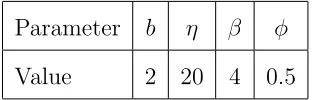
The benchmark values for other parameters are as follows.
Parameter b η β φ
Value 2 20 4 0.5
Except φ these values were not chosen on empirical grounds. In a detailed survey
of the Indian labour force Bhalla and Kaur [2011] estimate the unadjusted ratio of
female to male wages as approximately 0.58, and the value of φ is an approximation
[image:34.612.224.381.255.305.2]of that.
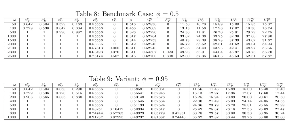
Figure 2 depicts the results for the benchmark case. The numerical values on which
Figure 2 is based are listed in the Appendix, Table 8. This should be consulted in
conjunction with Figure 2.
The top left panel of Figure 2 depicts male and female labour supply and education
levels for single agents. The other three panels depict only outcomes for married
females, since males are by construction restricted to market work in these examples.
The top right panel shows the female’s education and labour supply when marriage
formation is exogenous. The bottom left panel depicts the corresponding outcomes
along with her share of the market good when marriage is consensual. The bottom
right panel magnifies the details of the female education choice in the latter case. In
each panel, the horizontal axis measures the market wage.
We also studied a variant of the benchmark model with almost no labour market
Figure 2: Single, exogenous and consensual marriage.
Appendix, Table 9. The results were qualitatively similar to the benchmark case and
the quantitative differences were in line with expectation: a reduction in the degree
of wage inequality will, all else equal, promote female education and labour market
participation in all marital states and induce a married female’s entry into the labour
force at a lower wage.
Some noteworthy features of the results:
1) The education and labour supply of the female’s single self is greater than that
of both her married selves at each wage. At low wages, mutual specialisation occurs
under each marital arrangement. when this happens, the education level of a
con-sensually married female tends to lie below that of her exogenously married self, as
anticipated in the previous section.
2) So long as a married female supplies no labour, her education steadily decreases
once her labour supply becomes positive. This is the key effect of this section and
is consistent with Proposition 5. In the case of exogenous marriage formation her
educational level remains constant throughout the specialisation regime. This is
because in an exogenously formed marriage, her education depends on the wage only
if she supplies market labour,while in consensual marriage her education affects her
relative bargaining power even when she specialises in housework
3) As the underlying wage increases, a housewife’s share of the market good follows
the same declining pattern as her education. This is also in line with Proposition 5.
4) The threshold wage at which a consensually married female enters the labour
market is approximately ω = 2300 in the benchmark version. In the case of a female
in an exogenously formed marriage, this threshold arises at a slightly lower level of
the underlying wage: ω = 2100.
5) Once the threshold level of ω is crossed, the female’s education level appears to
jump up discontinuously and from there to increase with further increases in the
wage. These results should be treated as illustrative, emerging as they do from
numerical simulations and specific functional forms. The intuition behind the latter
effect is that once a female begins to provide positive amounts of labour, she is
able to meet the male’s selection constraint, as represented on the right-hand side of
equation (13), partly by earning market income. Thus, in her educational decision,
the balance shifts towards acquiring greater market skills. Note also that the female
share in consumption begins to increase once this threshold has been crossed (see
Table 8). The apparent discontinuity is likely to be driven by functional forms along
with the discrete nature of the manner in which wages are increased throughout the
simulation.27
27Comparing equation (14), the first-order condition for female education for a married female who
6) Although not depicted in the diagrams, the utility levels of the two spouses move
opposite to each other when comparisons are made between exogenous marriage
formation (with equal shares) and consensual marriage. For the benchmark case,
Appendix Table 8 shows that female utility is greater under exogenous marriage
formation than under consensual marriage. However when the degree of wage
dis-crimination is low, (φ = 0.95) her utility from consensual marriage may be higher or
lower than from exogenously formed marriage: the former is higher at low wages but
the latter becomes higher at high wages. For the male the comparisons go the other
way. These results suggest that despite the discontinuity in the effect of even a small
degree of wage inequality on the marital division of labour, a reduction in inequality
can enhance the female’s bargaining power within the household by increasing her
outside option to a level close to that of her prospective partner.
The key result of this section is that consensual marriage can lead to a negative
pres-sure on female education, and this prespres-sure might increase with increasing market
wages when the female specialises in housework. The reason is that when marriage
is subject to mutual selection constraints, an increase in the market wage can
dispro-portionately increase the male’s outside option relative to the female’s. Faced with
this, the female hedges between accepting a lower consumption share and choosing
less education, thus moving closer to the absolute maximum in terms of housekeeping
skills. This effect is reversed once she starts to contribute to the household’s market
income. At the same time, a reduction in wage discrimination (or an increase in
female wages alone) increases a consensually married female’s bargaining power even
when she does no market work and this increases her education and share of the
consumption good at given male wages.
7
A competitive marriage market:
We have thus far assumed that there is only one agent of each gender. This
pre-cludes the possibility of agents having a choice over partners. As Chiappori et. al.
[2009] have shown, marital choice matters for both the intra-household allocation of
rivalrous resources and each agents’ex ante investment in schooling. Choice expands
each agent’s set of outside options and opens each pre-nuptial negotiation to
compe-tition from potential rivals. Since we are analysing the interaction between marital
selection and female education it is instructive to see the effect of competition on this
interaction.
We extend the model by introducing an additional male and an additional female, one
or both of whom differ from the original pair in at least one attribute. All attributes
are, as before, common knowledge. Index agents belonging to the same gender as
1 and 2 and suppose that the matching process is complete, i.e. both types of one
gender may match with both types of the other. As in the previous section, we restrict
our analysis to cases in which there is mutual specialisation in time use by married
couples. Hence, the total amount of the market good available to a married couple
depends only on the exogenous male wage and its total output of the household good
depends only on the wife’s homemaking skills.
Let (Xi, Yj) denote a couple formed by male Xi and female Yj, i, j ={1,2}. Lete ij Yj
be Yj0s optimal educational choice when married to Xi and µij be Yj0s equilibrium
share of the consumption good in that match. The pair (eijY
j, µ
ij) is defined as the
household profile of (Xi, Yj) and it completely determines the utility levels of both
partners in (Xi, Yj). Thus UXiji = UXi(e
ij Yj, µ
ij) and Uij
Yj = UYj(e
ij Yj, µ
{(Xi, Yj),(Xh, Yk)} denote a matching pattern which assigns each individual to one
and only one couple, Xi, Xh ∈ {X1, X2}, i6=h; Yj, Yk ∈ {Y1, Y2}, j 6=k.
A stable matching pattern is an assignment {(Xi, Yj),(Xh, Yk)} that, given its
asso-ciated profiles {(eijY
j, µ
ij), (ehk Yk, µ
hk)}satisfies
(A) : UXij
i ≥U
s Xi; U
ij Yj ≥U
s Yj
Uhk Xh ≥U
s Xh, U
hk Yk ≥U
s Yk
and
(B) : 6 ∃ any feasible profiles (˜eik Yk,µ˜
ik),(˜ehj Yj,µ˜
hk)
associated with alternative couples (Xi, Yk) or (Xh, Yj)} that satisfy
(i) Uik Xi(˜e
ik Yk,µ˜
ik) ≥ Uij
Xi and U
ik Yk(˜e
ik Yk,µ˜
ik) ≥ Uhk Yk; or
ii UXhj
h(˜e
hj Yj,µ˜
hj) ≥ Uhk
Xh and U
hj Yj(˜e
hj Yj,µ˜
hj) ≥ Uij Yj
with “>” for at least one of the inequalities.
(A) ensures that each agent willingly enters into marriage. (B) ensures that there are
no feasible deviations from the candidate assignment and its associated profiles that
result in at least one partner in the deviating couple being made better off, with the
other no worse off, than under the candidate assignment.28 If (B) fails, then at least
one couple would mutually benefit by breaking away from their assigned partners.
Unlike matching models of non-transferable utility, such as Adachi [2003], in our
model each agent’s ranking of potential partners is endogenous, depending on both the
absolute size and the division of the surplus that their union is capable of generating.
In particular, the division of the rivalrous good depends on each partner’s outside
28This definition is adapted from Definition 5.2 in Adachi [2003] who shows that equilibrium
options, but these in turn depend on the surpluses and shares possible with rival
candidates. Thus preferences and outcomes are mutually dependent in our model.
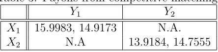
We therefore follow a step-wise procedure in solving the matching problem. First,
we construct a matrix of household profiles and payoffs by arbitrarily matching each
male with each female. At this stage, we ignore the possibility of competition from
rival candidates. This effectively makes the outside option of each partner exogenous
and equal to their utility from remaining single at this stage.29
The resulting utility levels are then used to generate a preliminary ranking of each
agent’s preferences over three outcomes: marriage to partner 1, marriage to partner
2 and staying single. At this point, a number of different possible combinations of
rankings can arise. Rather than an exhaustive analysis of these combinations, we
focus on two combinations that are both relevant to the aims of this paper and lend
themselves to examples based on simple modifications of the specification introduced
in the previous section.
7.1
Preferred couple:
The first combination is one in which the preliminary ranking results in one male and
one female being unanimously preferred over their respective rival. Without loss of
generality, suppose that these are X1 and Y1 respectively. The rankings for this case
are:
UY1j
j ≥U 2j Yj ≥U
s
Yj (20)
29Although this scenario is introduced only as a first step in identifying a stable matching pattern,