Integrating battery banks to wind farms for frequency support provision–capacity sizing and support algorithms

Integrating battery banks to wind farms for frequency support

provision–capacity sizing and support algorithms

A. B. Attya1

1

Department of Electronic and Electrical Engineering, University of Strathclyde, Glasgow, G1 1RD,

United Kingdom

The expected high penetration levels of wind energy in power systems require robust and

practical solutions to maintain typical conventional systems performance. Wind farms (WFs)

positive contribution in eliminating grid frequency deviations still a grey area, especially

when they replace considerable conventional generation capacities. This paper offers a sizing

algorithm to integrate storage battery banks (SBs) in WFs to provide feasible power support

during frequency events. This algorithm determines the required rated power and capacity of

each SB inside a WF according to several constrains, including wind speed characteristics at

WF location. The size of the SB is based on a statistical study for the amounts of rejected

wind power, and the events of low wind production. The offered operation algorithm controls

the SB charging, discharging, and standby modes based on the acquisition of different

dynamic variables, for example, WF output, load demand and storage cells’ state of charge.

The operation algorithm aims to mitigate frequency drops, rejected wind power and maintain

the battery lifetime. Both algorithms are applied on a defined sector from a genuine

conventional system merged with real WS chronological records at certain locations which

are candidates to host WFs. Results reveal the positive influence of SB involvement on

frequency excursions clearance, in addition, wasted wind energy is mitigated since wind

turbines de-loading techniques are avoided and some rejected wind power is utilized to

charge the installed SBs. Precise models are integrated through MATLAB and Simulink

simulation environment.

Key words— Wind power, Battery banks, Frequency drops.

Nomenclature

WT Wind Turbine

WF Wind Farm

DFIG Double Fed Induction Generator

SB Storage bank

SOC State of charge (max and min suffixes refer to its maximum and

minimum values respectively)

MPT Maximum power tracking operation technique

CC Conventional capacity in MW

CGC Conventional generation contribution (suffices: r: required, min:

minimum)

SCF1st Storage contribution factor using first method SCF2nd Storage contribution factor using second method WSi Instantaneous wind speed at the wind farm

WSi-avg Average wind speed at the wind farm number (i) location within certain duration (1 year in this paper)

WSrated Wind turbine rated wind speed

NWTk Number of installed WTs of the same type ‘k’ in the same WF

PWTk Rated power of WT type ‘k’

mi Number of installed WTs’ types in the same WF number (i).

M Number of connected WFs

CNi Number of cells in storage bank 'i'

∆PCtotal Total average charging power rating

∆Pch Charging power step of one cell

∆f Frequency deviation

Ci Storage bank 'i' ampere hour capacity

Loadinst. Instantaneous Load Demand

∆Pdisch i Discharge power step of storage bank 'i'

TS Continuous storage support time

Vci, Ici rated voltage and current of storage cell of bank ‘i’ respectively.

1. Introduction

Wind integration in modern power systems is presently one of the most active research fields.

Several risks are currently facing conventional energy generation, namely, depleted

resources, high fossil fuels prices and pollutant emissions. However, all renewable energies

face many obstacles avoiding high penetration levels in conventional grids. For example,

wind energy high penetration levels reduce system inertia and imply ambiguous impacts on

primary reserves [1]. Therefore, research efforts are directed towards simulating and

Thereupon, these research works offer practical solutions to overcome possible drawbacks

caused by wind energy integration.

The next paragraphs discuss the different methods offered in literature to enhance and

emphasis the role played by WFs in frequency deviations elimination. Most of these methods

count on wind turbine (WT) over speeding and/or de-loading. As an illustration, running the

WT at higher rotational speed than its optimum value (i.e. determined according MPT [4]),

makes its rotating parts store more kinetic energy. Thus, certain ratio from this kinetic energy

is extracted using different control methods by decelerating the WT to certain threshold

minimum rotational speed [5, 6]. The impact of conventional generators replacement by WFs

on overall system inertia was studied in [7]. It concluded that DFIGs penetration in power

system does not affect its total inertia if no conventional plants are displaced. Additionally, an

interesting conclusive comparison is offered in [8] between controlling WT as a conventional

generator using droop theory from one side to virtual inertia principle on the other side. On

the other hand, WT de-loading can be applied using pitch angle control so that WT output

power is de-rated below its optimum value. Consequently, the difference between optimum

and de-loaded outputs acts as a backup to suppress any sudden deviation between load

demand and generation [9]. Nevertheless, the feasibility of such method depends on the

precision and speed of pitching system controller and mechanics, as well as the accuracy of

wind speed (WS) measurements. The author has provided another algorithm which integrates

between most of WT support algorithms during frequency events. Initial version of this

algorithm is presented in [10] where support process is managed by WS categories to avoid

continuous de-loading at sufficient WSs.

Through the previous discussion, WT operation deviates from MPT operation; hence some

energy is wasted to provide acceptable support to the grid at frequency drops. In addition,

WFs reactions are always ambiguous according to WS conditions before, during and after the

frequency event. For example, at high WSs, the system is supported for longer times and the

probability of second frequency drop is lessened. Conversely, the system frequency

fluctuations and the probability of suffering a second drop increase at low WSs conditions.

Furthermore, WT inertia and aerodynamics have a deep influence on WT participation in

system frequency recovery. Therefore, integrating energy storage methods to provide the

required power support seems to be more appropriate.

Literature presented several types of energy storage methods, namely, batteries banks, hydro

storage to provide a predetermined power surge in case of frequency events. In addition, the

author has already examined hydro-pumped storage as source for frequency support [12].

An optimization technique counting on cost and low resolution WS data is performed through

Fuzzy logic and simple artificial neural network [13]. Predetermined threshold value for the

error between WFs forecasted output and actual output is selected to govern the

charging/discharging process. Likewise, an inspiring algorithm depends on the same error

definition in hourly forecasted power but with higher acceptable limit (i.e. up to 50%) is

presented in [14]. This research work did not concentrate so much on storage size estimation

but cared more for minimizing any financial penalties that might be implied on WFs’ owners

if WFs output power deviated beyond certain limit according to Hungarian grid code. On the

other hand, some literatures were much interested in analyzing the internal parameters

performance for battery bank cells, namely, current and voltage [15, 16]. The most promising

part was implementing a detailed model for NaS (Sodium Sulfur) and Li-ion batteries; hence

the obtained results were highly feasible and relevant. On the same track, battery voltage was

governed and total number of cells was estimated such that a maximum limit of

charging/discharging power is maintained [17].

Generally, the mentioned literatures utilized battery storage as a solution only for the negative

influence of WS intermittent nature on output power fluctuations. In words, dispatching WF

output to fulfill the required grid operators’ expectations was the main target. However, there

was no solid trial to exploit installed battery banks as a backup source for energy in case of

frequency excursions to provide a positive support in analogy to conventional plants

reactions. Three main topics should be discussed in this field, markedly, battery bank sizing,

charge/discharge control and the expected impact on system frequency. The required storage

capacity estimation is related to probabilistic forecasting for WS at certain location. In

addition, the capacity design aim to optimize the depth of discharge (DOD) such that battery

life is intensively extended [18]. The charging and discharging durations are also considered

to judge the required ampere hour capacity to allow the extraction of all stored energy at

certain power level.

This paper aims two targets; estimating the required storage capacity for each WF, and

controlling the SB charging-discharging procedure to provide reliable and feasible frequency

support. Driving the SB through charging process during wind energy rejection (i.e. the word

‘rejection’ refers to the presence of excess wind energy rejected by the grid according to

certain criterion as explained later) and discharging it during frequency events are innovative

any grid. As an illustration, the sizing algorithm requires chronological data for WS (or wind

power production), load demand, and the generation could be assumed fully reliable, as the

case in this paper or their outage data could be involved. In addition, the types and numbers

of WTGs inside each WF and the basic technical specifications of the installed SBs are

required. These data are available for any grid and any WF at different levels of time

resolution and accuracy. On the other hand, the dual-mode operation algorithm could be

applied to any SB. The requirements are instantaneous measurements for the WF production

and the grid load demand. The other signals are already required for any control method (e.g.

SOC and ∆f). Moreover, it does not require special control on WTs and it provides a fixed

predetermined power support at any frequency event.

The implied test system is a medium sized sector from a real system, namely, the Egyptian

grid so that the merits, drawbacks and possible further modifications are identified.

This paper is composed of seven sections including this introduction. Next section presents

the applied storage bank sizing algorithm while the third section explains SB control

procedure. Fourth section summarizes essential data about the concerned hypothetical test

system and the candidate locations for WFs construction. Case studies are described in

section five. Results are conducted in sixth section accompanied with a comprehensive

discussion, finally, Section seven concludes.

2. Assessment of storage bank rated power

Sizing of SB should compromise between economical side and technical aspects. However,

this paper concentrates on technical side such that the negative impacts of high wind energy

penetration levels are mitigated. Proposed algorithm acknowledges WS chronological records

in WF location and the acceptable level of conventional generation participation in load

coverage (i.e. generation mix) at normal operation. In other words, the amount of rejected

wind energy is related to maintaining the participation ratio of conventional generation within

certain boundary according to dynamic acquisition for load and WFs output variations.

The next steps describes implemented algorithm to determine the maximum possible

expected charging power, thereupon the required rated power and capacity of the SB:

1. WS data at specified site are obtained in acceptable time resolution (e.g. high resolution

means average WS value every 20 or 30 s) based on the actual WSs records within the

considered time span (e.g. 1 day). It is of note that, the WS or WFs output forecasting is out

or historical records of moderate resolution (the obtained SB size is altered based on the

accuracy and the resolution of the available data).

2. WS arrays are incorporated with WFs’ models to get WFs’ output power arrays. In this

paper, WS is assumed to be typical through the whole WF. Thus, the aggregation of installed

WTs equals the output of any WT multiplied by the number of WTs inside the WF.

3. Required conventional generation contribution in load feed (CGCr) is selected which is a

percentage from total conventional capacity (Cc). For example, when CGCr = 70%,

conventional generation output fluctuates around this value during normal operation,

according to the received control signals regarding load and WFs output discrepancies.

Generally, the CGCmin is decided by system operators (in this paper, WFs output participation

in load feeding should not exceed 50%). As an illustration, instantaneous wind power

penetration in generation mix should not increase above certain levels to maintain system

inertia and reserve [1]. When WFs outputs are high so that CGCmin is violated, excess wind

energy is rejected by the system. The power rejection takes place through the reduction of

WTGs output by violating the MPT conditions; however, this is not from the paper interests.

In the simulation model a limiter is integrated to insure that the WF instantaneous output is

not violating maximum allowed penetration ratio with respect to the demand. It is of note

that, conventional contribution in load feed is controlled based on load demand variations.

And according to the adjusted thresholds (i.e., CGCr and CGCmin), the process of wind power

storage and rejection is supervised.

4. Expected chronological load data should be available within the examined time span.

Afterwards, the events at which the load is greater than desired conventional generation

contribution (i.e. GCGr*Cc) are gathered in “Array1” using Eq(1). Note that, Array 1 keeps the time instant at which each event occurred. Thereupon, each instant in resultant array from

the previous step is subtracted from the corresponding output power of all integrated WFs at

the same instant using Eq(2). Hence, the positive events in Array 2 refer to WFs rejected power which could be imposed to charge battery banks. Thus, SB energy capacity and rated power could be estimated. It is worth mentioning that, low CGCr leads to remarkable

reduction in the density of rejection events as shown later.

Array 1 = Negative values of (Load-CC ∙ CGCr) Eq(1)

Array 2 = Positive values of (WFs output – |Array1|) Eq(2)

5. The average of rejected power events obtained in Step 4 is calculated to get an initial value

for SBs power rating based on the average charging power rating (∆PCtotal). Nevertheless, it

economic reasons. Most probably this rejected energy will not be fully utilized (i.e., when it

is stored) as demonstrated by mentioned literatures. Therefore, the expected rejected power

should be reduced by a roughly assumed ratio, namely, 20% as in this paper. This percentage

is inspired by some outcomes of previous literature. However, this reduction ratio could be

accurately evaluated using probability studies (e.g. Monte Carlo Simulation).

A distributed hybrid system (SB for each WF) is implemented instead of one large

centralized SB. This returns to the higher reliability of this pattern and the reduced losses,

where each SB is charged directly from the adjacent WF (i.e. losses due to charging power

transmission is almost avoided). In addition, the charging of SB is only dependent on its SOC

and the WF generation. Moreover, during frequency events in real system, when the

supporting active power is injected from diversely allocated plants the frequency recovery is

smoothed. The precise location of the SB inside the WF doesn’t have a major impact on its

role of supporting system during frequency drops. However, it is preferred to construct SB

hangar near the substation which connects the WF to the grid (point of common coupling).

The rated power of each SB is estimated through a fixed ratio called Storage Contribution

Factor (SCFi). The parameter SCF is an innovation for this paper. It is a simple parameter to distribute the overall required storage capacity between the connected WFs. Thereupon; SCFi

is multiplied by ∆PCtotal to get the required rated power of the installed SB at each WF. Two

procedures are suggested to evaluate SCF:

In the first method, SCFi1st is evaluated using Eq(3).

* * 1 1 * * 1 1 ( ) st k m

i avg k k

rated k k

i i

M _{k m}

i avg k k

rated k k

i i

WS _{PWT NWT}

WS m

SCF

WS _{PWT NWT}

WS m          



This formula is evaluated according to the participation of each ‘WTk’ type (i.e. ratio between

the number and rating of each WT type with respect to other types installed in the same WF).

Then a resultant value is obtained for all WTs types taking into consideration the annual

average WS at the WF location. This simplified method is applied to minimize further

simulation and computational efforts (compared to second method as shown next).

Second method counts on WFs output power arrays obtained in the second step of the main

algorithm. Particularly, at each time step the WFi output power is divided on the overall WFs

output. Afterwards, an average value for all ratios within the considered time span is

calculated (SCF2ndi). However, this algorithm requires enormous simulation and

is applied only on four specific days, markedly, the days of highest average loads in each

weather season as shown in Table (1).

Finally, a compromise between the two methods is applied using Eq(4). This compromise is

applicable since the considered time span (i.e. 4 days) is relatively short, so that both methods

are computationally feasible. Moreover, integrating the two methods reduces possible higher

error in the first one. However, literature has also calculated storage power ratings using other

simplified methods. For example, the storage power rating is a fixed percentage from WF

overall capacity, namely, 10-15% according to the results obtained in [16, 17].





1 2

i

1 2

1

SCF



 





st nd

st nd

i i

M

i i

i

SCF SCF

SCF SCF

Eq(4)

The number of battery cells required for each WF SB is estimated based on the power rating

of the selected cell type. Consequently, the number of cells (CNi) composing each SB is

obtained. An illustrative flowchart for the prosed sizing algorithm is displayed in Figure 1.

Figure 1 Sizing algorithm flowchart

Table 1 Four sample days according to Egyptian load data

Season Winter Spring Summer Fall 24Hrs average load, GW 14.9 13.2 14.6 16.3

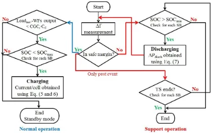
3. Battery bank operation

Proposed algorithm splits into Normal and Support operation and it depends on four control

signals, markedly, load demand, WFs output power, SOC and frequency deviation (∆f).

3.1 Normal Operation

Two possibilities are considered in this operation region, namely, charging and standby (i.e.

neither charging nor discharging) modes. Charging activation requires the overlap of the

following conditions:

 SOCmin ≤ SOC < SOCmax

 [(Loadinst. - CGCr·CC)·SCFi] > WFi output (i.e. the presence of excess power in WFi)

SCFi has a different application in second condition since it represents the expected share of

WFi in load coverage. The monitoring of the second condition requires a compact data

acquisition system which receives instantaneous load (Loadinst.) and WFi output in a

reasonable time step. The selection of SOCmax and SOCmin is related to DOD which has a

severe impact on battery lifetime [13]. The SB is charged with a power step (∆Pch) obtained

using Eq(5). ∆Pch is handled by certain number of AC/DC converters as shown in Figure 2. It

is of note that during charging the SB the WF continues feeding the grid with certain amount

of power decided by (5), where it is the negative component of the left hand side.

.

- ( - ) /

ch i i inst C i i

P WF output Load CGC C SCF CN

    Eq(5)

Nevertheless, the share of each storage cell from ∆Pch should not violate the rated current and

voltage of the installed cell type. Particularly, when the output of WF is high so that ∆Pch

violates SB ratings; the extra power is directed to feed the existing load; hence, CGCr is

decreased below its predetermined value. Thus, conventional generators output is reduced, in

parallel with suitable adjustments in the converters which control the power flow from WF to

grid and SB. Hence, the amounts of wasted or rejected wind power are reduced. The number

of integrated converters counts on the ratings and available budget for power electronics

devices. Some literature preferred a single converter for each group of cells; in other

approaches; one converter (i.e. DC/AC) ties between the SB and the power system. For

simulation simplicity, the ∆Pch is interpreted into a charging DC current fed into the storage

cell model using Eq(6), where Vci and Ici are the rated voltage and current of SB cell

respectively. It is worth mentioning that, the minor losses and time delays of power

ch

charging charging

P

; ci

ci i

i i I

V CN



 

 Eq(6)

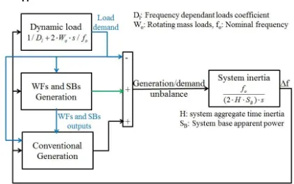
Figure 2 Major blocks and control signals of wind generation and storage bank

3.2 Support Operation

Support operation is activated when ∆f violates a predetermined limit based on grid operators

requirement (in this paper ∆f safe margin is -0.05 Hz [19]) as long as SOC > SOCmin.

Throughout Support mode, all WFs’ outputs are exploited to cover load demand i even if

CGCr predetermined value is violated. The provided power step is considered to be constant

(∆Pdisch) to curtail generation-demand mismatch. ∆Pdisch-iis obtained using Eq(7).

=

disch i i i i total i

P Vc Ic CN PC SCF

      Eq(7)

Most of the highlighted support techniques based on WTs' stored kinetic energies face the

risk of causing a second frequency deviation after the depletion of extracted kinetic energy.

On the contrary, SBs have fixed predetermined participation for certain defined duration (i.e.

∆Pdisch i continues for certain time (TSi) to reduce the occurrence probability of a second frequency excursion). TS starts counting when ∆f reaches its safety margin for the first time

after a frequency event and it is reset when ∆f violates its safety limit. However, TS

completion depends on SOC value such that it is forbidden to violate SOCmin in order to

complete TS. TSi is adjusted on a proportional basis to CNi using Eq(8) to dispatch the WFs’

contributions. Thus, the switching of all WFs from Support to Normal operation is not

synchronized to mitigate the risks of successive frequency events and incident fluctuations.

that all the cells are typical in all SBs. TSlongest value is predetermined by operators (i.e. it is

assumed to be 90s in this paper to be relevant to the average clearance duration of moderate

frequency deviations), accordingly other TS values are evaluated.

i

i longest

highest.

CN

TS TS

CN

  Eq(8)

An illustrative flowchart for the prosed operation algorithm is displayed in Figure 3.

Figure 3 Operation algorithm flowchart

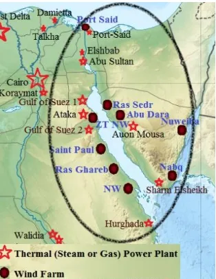
4. Test system

The benchmark system implemented in this research work is inspired from certain sector

from the Egyptian 50 Hz grid as shown in Figure 4. The selection of Egyptian grid returns to

the funding of Egyptian ministry of higher education and research to part of the presented

work. It is of note that the mentioned data is related to the year 2010 (the start of the research

project). Considered sector is unique due to the concentration of nine WFs candidate

locations within a small geographical area so that they could be easily linked with the nearby

conventional plants. CC before wind energy integration is 3825 MW as indicated in Table (2).

Generally, the accurate estimation for wind energy capacity could not be achieved due to WS

intermittent nature. The actual capacity based on probabilistic and chronological estimations

was in range of 25 to 45% [20]. Meanwhile, according to practical estimation in relevance to

WSs records and WFs specifications in certain region, the actual capacity reached 55% [21].

rated powers, markedly, 1024 MW. Thus, new CC is 2801MW and the average wind power

penetration is 27% from the former CC.

Nine WFs, whose locations and WSavg are described in Table (2) [22], replace certain portion

from the former conventional capacity. Two types of WTs are integrated, namely, GE-1.5

MW and G-2 MW such that each WF includes 65 units from each type. For simplicity, and

since there is no special control algorithms are integrated to the WT (i.e. all WTs follow their

MPT curves), the production of both types of WTs is anticipated based one the incident WS

and MPT look-up table of each type which are published by the manufacturers [23, 24].

The available WS data in each location are average WSs records every ten minutes [25]. The

methodology presented in [26] is applied to get higher resolution WSs arrays, namely, 15 s

time step so that the impact of WS dynamics is acknowledged.

The Egyptian grid chronological hourly load is integrated after it is de-rated by 79.9% (i.e.

ratio between the concerned sector generation capacity to the whole grid capacity is 20.1%).

Selected block diagrams for the integrated simulation models are present in the Appendix.

Further information is found in the related references.

Figure 4 Involved Egyptian grid sector and WFs’ locations

Table 2 Integrated conventional Plants and WFs No. WF location WSavg.

5. Case Studies

Base case study analyzes the system frequency response during two successive frequency

excursions caused by sudden rise in load demand by 8% from its actual amount (i.e. 2838

MW) then it rises steeply again after 45 s by an additional 3%. System frequency simulation

is based on the method conducted in [27]. The sudden increase in load is applied to initiate a

frequency drop event. The author preferred to keep the installed generation capacity

unchanged during the event; hence the frequency drop is not initiated by a sudden generation

outage. In addition, the cause of frequency drop will not have an impact on the SBs support

(because the support is triggered according to ∆f violation which occurs in both cases), and

the impact on the frequency response will be very minor.

The under-loading events are not of interest for this paper as they will cause positive

frequency deviations and this is already handled in the grids by the reduction of WFs output

through certain ramps defined by grid codes. In addition, the charging of SBs in the proposed

algorithm is not related to frequency (except if the system is suffering a drop, charging halts),

and this to avoid the intensive switching between charging/no charging due to rapid

frequency fluctuations (to maintain the battery lifetime).

First and second case studies examine frequency responses after WFs integration without and

with SBs installation respectively. Benchmark system single line diagram is displayed in

Figure 5. It should be highlighted that the WTs operation in both cases is following the

traditional MPT, and the harvested wind energy is fed to load (and charge the SB) or rejected

according to the algorithm explained previously.

Figure 6 describes ∆PCtotal variation depending on CGCr value selection in the proposed

algorithm. ∆PCtotal is escalating almost linearly with the increase of CGCr. As an illustration,

the rising of CGCr expands wind power rejection possibility, thus more power is available to

charge the SBs. Noticeable divergence between the four sample days returns to different WSs

conditions in all WFs and the chronological load demand. The spring day results are excluded

from calculating ∆PCtotal average value due to the odd and very low expected rejected power

in that specific day which might be misleading to the whole performance during Spring.

However, ∆PCtotal average value for the other three days at CGCr =70% is implied in this

paper (i.e. ∆PCtotal = 178 MW equivalent to 4.7% from the sector generation capacity, and

8.7% from the installed wind power capacity).

In this research work, only one type of storage cells is exploited for all SBs, namely, Trojan

assumed to be 55%; hence battery type lifetime should be obviously extended according to

fabricator recommendations. Consequently, SOCmax = 85% and SOCmin = 30% while the

initial SOC in all case studies is assumed to be 70%. The universal battery model, embedded

in Simulink and inspired from [29], is implemented to simulate accurate SB cells responses

including the storage units’ losses.

SB sizing algorithm is applied on the four sample days, providing four various values for

∆PCtotal, SCF2nd at each day hence, an average value is calculated for each factor as shown in

Table (4). However, the error between SCF1st and SCF2nd is considerable and it basically depends on the selected time span to perform the proposed sizing algorithm. The hangars

areas are calculated using Eq(9), and included in Table (4).

For instance, it is assumed that all the hangars have the same height, namely, 10 m, thereupon

12 cells could be aligned vertically allowing an overall tolerance between cells of 30%.

Meanwhile, the extra spacing in the horizontal distribution of cells columns and human

corridors is 160% from the exact area of the horizontally spreading cells. The outcome

hangar areas seem to be reasonable, especially, if compared to either substations areas or the

huge WFs terrains.

2.6 12

i i

CN

Hangar area  cell base area Eq(9)

The winter day data is selected to execute mentioned case studies since it recorded the

highest superfluous of wind power. Thus, the proposed algorithm is examined at high wind

energy penetration level. The simulation time for each case is one hour, namely, from 6 to

7pm since the load is relatively high and the wind power is moderate within this duration.

Control signals concerning load variations and ∆f which are fed to conventional plants’

governors are delayed by 20 s after the first frequency event starts. This delay emphasizes the

Figure 5 Benchmark system single line diagram

Figure 6 ∆PCtotal vs. CGCr at the four indicated sample days

Table 3 Integrated (L16RE-B) battery cell technical aspects Rated power C Rated voltage Rated current Base area Height

2.46 kW 410 A.H 6V 410A 1763 cm2 61 cm

Table 4 WFs storage banks basic parameters

WF location SCF1st SCF2nd Average SCF TS, s CN Hangar area, m2 ∆Pdisch, MW

Ras Ghareb 0.23 0.13 0.238 90 11531 441 42.31

NW 0.19 0.13 0.185 71 8969 343 32.91

This paper does not tackle the extreme case when the SOC is minimum and the system is

facing a frequency event. Actually, this is very rare to happen because it means that the WS

conditions were very poor in all the WFs for a long time, and the system has already faced

several frequency events during this time so that all the stored energy is depleted. However,

in this worst case scenario, the WTs might be equipped with certain support algorithm to

provide a slight active power surge, but this is out of the focus of this paper. It is of note that

this paper proposes a solution to make the WF have a defined amount of primary reserve of a

very low uncertainty compared to the support algorithms which are WTG-based.

6. Results and discussion

The base case study is considered to be a reference to judge the impact of wind energy

integration with and without SBs. In Figure 7, system frequency responses are displayed till

80 s after the first frequency event occurred. Practically, the frequency is oscillating all the

time within an accepted margin. The WFs output variations (based on the integrated WS

arrays) causes a continuous unbalance between generation and demand, hence the system

frequency is always oscillating in addition to the impact of the dynamic load model. Actually,

the frequency deviation will not reach zero in the integrated model because the WS is

changing every 15s, thus the generation-demand balance is interrupted most of the time.

However, the WS variations, leading to WFs output variations are not high enough to make

the frequency deviations violate the safe margin (50 mHz). In addition, this model doesn’t

provide secondary frequency response (i.e. AGC), thus the frequency will not reach exactly

its nominal value. However, the focus is drawn on the role of SB to provide primary response

during frequency dips, to compensate the high penetration level of wind power.

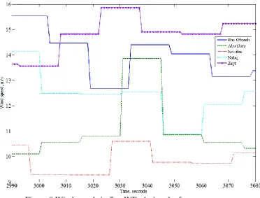
The forced delay in control signals of conventional plants’ governors is clear, such that the

frequency started its recovery after 20s in base case. However, the integration of WFs

accelerated the recovery process but it failed to reduce the maximum ∆f. As shown in Figure

8, the relatively high or moderate WS in some WFs during frequency excursions caused this

positive consequence. Meanwhile, the positive impact of SBs is clear since it mitigated the

maximum ∆f by 0.2 Hz and derived ∆f to its safety margin within 6 s compared to 22 s in

Case 1. Moreover, the resultant frequency fluctuations are not severe and could be handled.

In the second successive frequency event, the conventional generation reaction is not

delayed; hence, the recovery process starts earlier. Nevertheless, still the positive effect of

SBs is apparent such that the maximum ∆f is mitigated and it reaches its acceptable threshold

positive ∆f overshoot. In particular, the positive ∆f occurring after each frequency excursion

clearance is an expected result to the extra power fed by SBs within different TS duration. In

other words, the SBs injected powers continue even after ∆f reaches its acceptable value until

TS ends. As illustrated before, the independence of SB supporting power continuity on ∆f

caused this overshoot. To fix this problem, TSlongest could be shortened or ∆Pdisch is adjusted

dependently on ∆f instantaneous value through certain droop function. The overshoot could

also be reduced by integrating a supplement controller to the discharging process of SBs

during frequency events. The controller will manage the discharging current according to the

frequency deviation and/or the rate of change of frequency (RoCoF). In such way, the SBs

will not just be switched between No discharging/Rated power discharging, but the

discharging will vary smoothly according to the frequency event development. This could be

an interesting topic for further research. However, linking ∆Pdisch to ∆f might generate high

undeserved fluctuations in SBs output power leading to mitigated lifetime.

Comparing the improvements achieved in frequency responses with corresponding results in

some literatures (e.g. [7, 8]) reinforces the feasibility of presented SBs support algorithm.

Furthermore, these comparisons confirm that SBs transcend over several WTs support

algorithms, especially from the point of view of wasted wind energy curtailment in case of

SBs utilization since WTs’ complicated de-loading techniques are avoided.

Figure 8 Wind speeds in five WFs during the frequency events

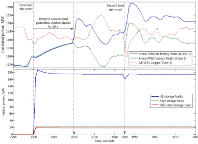
The generation variations during frequency drop clearance are considered in Figure 9. The

wind power penetration in generation mix at the instant of frequency is 48%. In spite of this

high WFs participation, the frequency attitude is not negatively affected, but it has slightly

improved. The conventional generation is obviously reduced in Case 2 compared to Case 1

due to SBs contribution. Additionally, there is almost no deviation between steam generation

curves in Cases 1 and 2. Conversely, when SBs are connected, conventional generation

supplies more power to compensate the power injected by WFs to charge their connected

SBs. As shown in Figure 10(a), all SBs reached SOCmax prior to the displayed time interval

within the simulated hour (i.e. Consider that the initial SOC is 70% as mentioned earlier).

The moderate WSs conditions during the considered simulation interval make the SBs get

Figure 9 Conventional, WFs and storage banks output powers

The outputs of selected SBs during frequency events are shown in Figure 9. Within the first

few seconds the overall output power of all SBs increases rapidly to a value (182 MW) higher

than the rated power of all SBs. This returns to the voltage transient response of installed

cells which implies voltage overshoots accompanied with rated currents causing this high

output. After few seconds, it settles down to its normal rated power of 178 MW. It faces an

intended decrease after 43 s because the TS of some SBs have run out, namely, Port Said and

Nweiba SBs as indicated in Table (4). As soon as the second frequency event hits, these two

SBs are switched again to Support mode and the TS is reset. It should be highlighted that the

major merit of SBs over other support techniques is accentuated under these severe

circumstances. As an illustration, in traditional support techniques, WTs require some time to

re-store kinetic energies and attain their normal rotational speeds; hence their chances to

provide further support in case of a second consecutive frequency event diminish.

Conversely, the SBs can interact positively to a second frequency deviation as long as SOC is

efficient whereas their reacting speed counts on the time constants of integrated batteries and

installed power electronics devices. In addition, offered SBs support algorithm does not

require any WS instantaneous measurements in comparison to many support techniques

which count on special control algorithms. Thus, it evades from the debate of possible errors

in such measurements and its possible negative influence on WTs support techniques

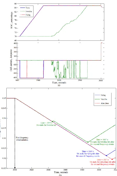
Figure 10 Selected batteries’ cells internal parameters performance

The internal performances of some selected cells are also concerned in this discussion as

depicted in Figure 10(b). In the proposed algorithm, the available extra wind power (i.e.

SOCs of all cells in the same SB are typical as shown in Figure 10(b). Nweiba SOC reached

its optimum value delayed compared to the other two SBs due to the poor WSs conditions,

hence the WF output is barely sufficient to cover its forecasted share in load coverage and the

charging power is restricted. At the excursion, all cells are discharging by the same rate

because ∆Pdisch is typical for all SBs. The same concept is insured by the

charging/discharging currents attitudes of the three different cells. In particular, the

discharging current is always fixed at its rated value to provide the pre-adjusted ∆Pdisch from

the whole SB. On the other hand, negative charging current is fluctuating according to WS

variations which determine how much excess power is available to charge the cell (e.g.

Nweiba SB). However, high WSs in Abu Dara and Nabq sites caused a fixed rated charging

current which is an advantage to the cell life span. Either during charging or discharging the

current is limited to its rated value to avoid any damage for the cells.

The steep changes in current variations are interpreted by the ignorance of power electronic

devices delays and their transitioning stages since they are short compared to the time

required by system inertial responses and frequency variations.

Figure 10(b) assures that different discharging periods are related to the pre-defined TS. The

Nweiba SB has the shortest TS (39 s) with respect to Abu Dara and Nabq SB. Regarding the

time instant at which ∆f reaches its safe margin after the first excursion, namely, at 3006 s,

the TSNweiba ends at 3045 s. Meanwhile, Abu Dara has longer TS (69 s), hence it does not end

after the first frequency event, since the second excursion occurs prior to TS completion.

However, it ends after ∆f stabilizes in the safe region (at 3048 s as shown in Figure 7). Thus,

Abu Dara discharging mode stops at time = 3048 + 69 = 3117 s as shown in Figure 10(b).

7. Conclusions

The presented research work deals with the impact of wind farms integration in power

systems on frequency response at frequency drops. Battery storage banks are utilized to

overcome possible drawbacks for high levels of wind power penetration in conventional

grids. This paper focused on providing a feasible and detailed algorithm to estimate the

power rating and energy capacity of required storage banks. Moreover, it offered a consistent

algorithm to drive the installed storage bank in each wind farm either during normal

operation conditions or during frequency drops. Both algorithms are implemented on certain

sector in the Egyptian grid using real wind speed data. Detailed analysis for frequency

responses, generation variations and cells’ internal parameters fluctuations is conducted.

algorithm on mitigating frequency excursions and the curtailment of required time to reach

frequency deviation safe margin.

The superiority of SBs over other direct support techniques (e.g. de-loading) lies in: 1-

avoiding of complicated controllers to apply de-loading or any other method, 2- avoiding

wasting power due to direct support algorithms which most probably lead to the violation of

MPT, 3- securing a predetermined amount of active power support (i.e. based on SB rating

and droop), not depending on the prevailing WS conditions, 4- WS measurements are not

required, 5- easier to dispatch, compared to the dispatching of WTGs inside the WF and

WFs’ dispatching.

In future work, improvements are planned including more complicated methods to control

discharging (i.e. support power) provided by each storage bank, mainly to mitigate the

possible post drop frequency deviation overshoot. Additionally, the longest continuous

storage support time should be better tuned through comprehensive experiments and

consistent with the frequency excursions history of the integrated grid sector. This algorithm

might be also merged with traditional methods which employ storage banks as economical

solutions to save wind energy during cheap tariff intervals.

8. Appendix

Figure A.2 Wind farm aggregate model

Figure A.3 Storage bank model

Figure A.4 Steam Turbine integrated governor

Table A.1 Integrated WTs types basic specifications

WT type GE 77 G 90

Manufacturer General Electric Gameza

Rotor diameter, m 77 90

Rated WS, m/s 13 16

Rated output, MW 1,5 2

rotational speed range, rad./s 1.15 -2.51 0.94 -1.99 Table A.2 Steam Turbine and governor data[30]

Parameter Value

T3, seconds 0.35

Max opening and closing rates, p.u./s 0.2, -0.1

Droop (RS) 3%

TCH, TR1, TR2 and TCO, seconds 0.25, 7.5, 7.5 and 0.4

9. References

1. Ye, W., et al., Methods for Assessing Available Wind Primary Power Reserve. Sustainable Energy, IEEE Transactions on, 2015. 6(1): p. 272-280.

2. Holttinen, H., et al., Currents of Change. IEEE Power & Energy Magazine, 2011. 9(6): p. 47-59. 3. B. Fox, et al., Wind Power Integration. IET Power and Energy Series. 2007: IET.

4. Z. Meng, An improved equivalent wind method for the aggregation of DFIG wind turbines, in IEEE International Conference on Power System Technology (POWERCON). 2010: China.

5. B. G. Rawn, M. Gibescu, and W. L. Kling, Kinetic Energy from Distributed Wind Farms: Technical Potential and Implications, in IEEE Innovative Smart Grid Technologies Conference Europe. 2010: Sweden.

6. Attya, A.B.T. and T. Hartkopf, Control and quantification of kinetic energy released by wind farms during power system frequency drops. Iet Renewable Power Generation, 2013. 7(3): p. 210-224. 7. Ruttledge, L., et al., Frequency Response of Power Systems With Variable Speed Wind Turbines. IEEE

Transactions on Sustainable Energy, 2012. 3(4): p. 683-691.

8. Margaris, I.D., et al., Frequency Control in Autonomous Power Systems With High Wind Power Penetration. IEEE Transactions on Sustainable Energy, 2012. 3(2): p. CP2-199.

9. Chang-Chien, L.-R. and Y.-C. Yin, Strategies for Operating Wind Power in a Similar Manner of Conventional Power Plant. IEEE Transactions on Energy Conversion, 2009. 24(4): p. 926-934. 10. Attya, A.B. and T. Hartkopf, Penetration impact of wind farms equipped with frequency variations ride

through algorithm on power system frequency response. International Journal of Electrical Power & Energy Systems, 2012. 40(1): p. 94-103.

11. Juan A. Martinez, Modeling and Characterization of Energy Storage Devices, in IEEE Power and Energy Society General Meeting. 2011: Detroit Michigan.

12. Attya, A.B. and T. Hartkopf, Utilizing stored wind energy by hydro-pumped storage to provide frequency support at high levels of wind energy penetration. Iet Generation Transmission & Distribution, 2015. Accepted.

13. Brekken, T.K.A., et al., Optimal Energy Storage Sizing and Control for Wind Power Applications.

IEEE Transactions on Sustainable Energy, 2011. 2(1): p. 69-77.

14. Hartmann, B. and A. Dan, Cooperation of a Grid-Connected Wind Farm and an Energy Storage Unit-Demonstration of a Simulation Tool. Ieee Transactions on Sustainable Energy, 2012. 3(1): p. 49-56. 15. Teleke, S., et al., Control Strategies for Battery Energy Storage for Wind Farm Dispatching. Ieee

Transactions on Energy Conversion, 2009. 24(3): p. 725-732.

16. Teleke, S., et al., Rule-Based Control of Battery Energy Storage for Dispatching Intermittent Renewable Sources. Ieee Transactions on Sustainable Energy, 2010. 1(3): p. 117-124.

17. Yao, D.L., et al., A Statistical Approach to the Design of a Dispatchable Wind Power-Battery Energy Storage System. Ieee Transactions on Energy Conversion, 2009. 24(4): p. 916-925.

18. Li, Q., et al., On the Determination of Battery Energy Storage Capacity and Short-Term Power Dispatch of a Wind Farm. IEEE Transactions on Sustainable Energy, 2011. 2(2): p. 148-158.

19. UCTE, Appendix 1 — Load-Frequency Control and Performance. 2002, The Union of the coordination of the transmission of electricity.

20. Castro, R.M.G. and L. Ferreira, A comparison between chronological and probabilistic methods to estimate wind power capacity credit. Ieee Transactions on Power Systems, 2001. 16(4): p. 904-909. 21. Gevorgian, V., Y. Zhang, and E. Ela, Investigating the Impacts of Wind Generation Participation in

Interconnection Frequency Response. IEEE Transactions on Sustainable Energy, 2014. PP(99): p. 1-9. 22. The annual report. 2010, Egyptian ministry of Electricity and Energy: Cairo.

23. Brochure of Wind Turbine: G-90-2.0 MW. 2011, Gameza Company: Spain.

24. Miller, N.W., et al., Dynamic modeling of GE 1.5 and 3.6 MW wind turbine-generators for stability simulations. 2003 Ieee Power Engineering Society General Meeting, Vols 1-4, Conference Proceedings, 2003: p. 1977-1983.

25. N. G. Mortensen and U.S. Said, Wind Atlas for Egypt. 2009, New and Renewable Energy Authority: Cairo.

26. Attya, A.B. and T. Hartkopf. Generation of high resolution wind speeds and wind speed arrays inside a wind farm based on real site data. in Electrical Power Quality and Utilisation (EPQU), 2011 11th International Conference on. 2011.

27. Kundur, P., Power System Stability and Control. 1994, New York: McGraw-Hill Inc.

28. Energy Storage Solutions for Renewable Energy series manual. 2012, Trojan Battery Company: USA. 29. Ceraolo, M., New dynamical models of lead-acid batteries. IEEE Transactions on Power Systems,

30. DYNAMIC MODELS FOR STEAM AND HYDRO TURBINES IN POWER-SYSTEM STUDIES. Ieee Transactions on Power Apparatus and Systems, 1973. PA92(6): p. 1904-1915.