Optimizing Laguerre expansion based deconvolution methods for analysing bi-exponential fluorescence lifetime images

Optimizing Laguerre expansion based

deconvolution methods for analysing

bi-exponential fluorescence lifetime images

Yongliang Zhang,1,2 _{Yu Chen,}3 _{and David Day-Uei Li}1,*

1_{Centre for Biophotonics, Strathclyde Institute of Pharmacy & Biomedical Sciences, University of Strathclyde,}

Glasgow, G4 0RE, Scotland, UK

2_{College of Information Science & Electronic Engineering, Zhejiang University, Hangzhou, 310007, China} 3_{Department of Physics, University of Strathclyde, Glasgow G4 0NG, Scotland, UK}

*_{David.Li@strath.ac.uk}

Abstract: Fast deconvolution is an essential step to calibrate instrument responses in big fluorescence lifetime imaging microscopy (FLIM) image analysis. This paper examined a computationally effective least squares deconvolution method based on Laguerre expansion (LSD-LE), recently developed for clinical diagnosis applications, and proposed new criteria for selecting Laguerre basis functions (LBFs) without considering the mutual orthonormalities between LBFs. Compared with the previously reported LSD-LE, the improved LSD-LE allows to use a higher laser repetition rate, reducing the acquisition time per measurement. Moreover, we extended it, for the first time, to analyze bi-exponential fluorescence decays for more general FLIM-FRET applications. The proposed method was tested on both synthesized bi-exponential and realistic FLIM data for studying the endocytosis of gold nanorods in Hek293 cells. Compared with the previously reported constrained LSD-LE, it shows promising results.

Published by The Optical Society under the terms of the Creative Commons Attribution 4.0 License. Further distribution of this work must maintain attribution to the author(s) and the published article’s title, journal citation, and DOI.

OCIS codes: (030.5260) Photon counting; (110.2960) Image analysis; (110.0180) Microscopy; (170.3650) Lifetime-based sensing; (170.6920) Time-resolved imaging.

References and links

1. K. Okabe, N. Inada, C. Gota, Y. Harada, T. Funatsu, and S. Uchiyama, “Intracellular temperature mapping with a fluorescent polymeric thermometer and fluorescence lifetime imaging microscopy,” Nat. Commun. 3, 705 (2012).

2. M. C. Skala, K. M. Riching, D. K. Bird, A. Gendron-Fitzpatrick, J. Eickhoff, K. W. Eliceiri, P. J. Keely, and N. Ramanujam, “In vivo multiphoton fluorescence lifetime imaging of protein-bound and free NADH in normal and pre-cancerous epithelia,” J. Biomed. Opt. 12, 024014 (2007).

3. D. M. Kavanagh, A. M. Smyth, K. J. Martin, A. Dun, E. R. Brown, S. Gordon, K. J. Smillie, L. H. Chamberlain, R. S. Wilson, L. Yang, W. Lu, M. A. Cousin, C. Rickman, and R. R. Duncan, “A molecular toggle after exocytosis sequesters the presynaptic syntaxin1a molecules involved in prior vesicle fusion,” Nat. Commun. 5, 5774 (2014).

4. V. Ntziachristos, “Going deeper than microscopy: the optical imaging frontier in biology,” Nat. Methods 7(8), 603–614 (2010).

5. S. P. Poland, A. T. Erdogan, N. Krstajić, J. Levitt, V. Devauges, R. J. Walker, D. D.-U. Li, S. M. Ameer-Beg, and R. K. Henderson, “New high-speed centre of mass method incorporating background subtraction for accurate determination of fluorescence lifetime,” Opt. Express 24(7), 6899–6915 (2016).

6. S. Coda, A. J. Thompson, G. T. Kennedy, K. L. Roche, L. Ayaru, D. S. Bansi, G. W. Stamp, A. V.

Thillainayagam, P. M. French, and C. Dunsby, “Fluorescence lifetime spectroscopy of tissue autofluorescence in normal and diseased colon measured ex vivo using a fiber-optic probe,” Biomed. Opt. Express 5(2), 515–538 (2014).

7. M. Y. Berezin and S. Achilefu, “Fluorescence lifetime measurements and biological imaging,” Chem. Rev.

110(5), 2641–2684 (2010).

9. J. Liu, Y. Sun, J. Qi, and L. Marcu, “A novel method for fast and robust estimation of fluorescence decay dynamics using constrained least-squares deconvolution with Laguerre expansion,” Phys. Med. Biol. 57(4), 843– 865 (2012).

10. A. Shivalingam, M. A. Izquierdo, A. L. Marois, A. Vyšniauskas, K. Suhling, M. K. Kuimova, and R. Vilar, “The interactions between a small molecule and G-quadruplexes are visualized by fluorescence lifetime imaging microscopy,” Nat. Commun. 6, 8178 (2015).

11. Y. Sun, C. Rombola, V. Jyothikumar, and A. Periasamy, “Förster resonance energy transfer microscopy and spectroscopy for localizing protein-protein interactions in living cells,” Cytometry A 83(9), 780–793 (2013). 12. A. Leray, S. Padilla-Parra, J. Roul, L. Héliot, and M. Tramier, “Spatio-temporal quantification of FRET in living

cells by fast time-domain FLIM: A comparative study of non-fitting methods [corrected],” PLoS One 8(7), e69335 (2013).

13. F. Fereidouni, G. A. Blab, and H. C. Gerritsen, “Phasor based analysis of FRET images recorded using spectrally resolved lifetime imaging,” Methods Appl. Fluoresc. 2(3), 035001 (2014).

14. E. M. Merzlyak, J. Goedhart, D. Shcherbo, M. E. Bulina, A. S. Shcheglov, A. F. Fradkov, A. Gaintzeva, K. A. Lukyanov, S. Lukyanov, T. W. Gadella, and D. M. Chudakov, “Bright monomeric red fluorescent protein with an extended fluorescence lifetime,” Nat. Methods 4(7), 555–557 (2007).

15. S. Padilla-Parra and M. Tramier, “FRET microscopy in the living cell: different approaches, strengths and weaknesses,” BioEssays 34(5), 369–376 (2012).

16. J. L. Rinnenthal, C. Börnchen, H. Radbruch, V. Andresen, A. Mossakowski, V. Siffrin, T. Seelemann, H. Spiecker, I. Moll, J. Herz, A. E. Hauser, F. Zipp, M. J. Behne, and R. Niesner, “Parallelized TCSPC for dynamic intravital fluorescence lifetime imaging: quantifying neuronal dysfunction in neuroinflammation,” PLoS One

8(4), e60100 (2013).

17. M. C. Morris, Fluorescence-Based Biosensors: From Concepts to Applications (Elsevier Science, 2012). 18. R. Niesner, B. Peker, P. Schlüsche, and K. H. Gericke, “Noniterative biexponential fluorescence lifetime

imaging in the investigation of cellular metabolism by means of NAD(P)H autofluorescence,” ChemPhysChem

5(8), 1141–1149 (2004).

19. C. Y. Fu, B. K. Ng, and S. G. Razul, “Fluorescence lifetime discrimination using expectation-maximization algorithm with joint deconvolution,” J. Biomed. Opt. 14(6), 064009 (2009).

20. K. C. Lee, J. Siegel, S. E. Webb, S. Lévêque-Fort, M. J. Cole, R. Jones, K. Dowling, M. J. Lever, and P. M. French, “Application of the stretched exponential function to fluorescence lifetime imaging,” Biophys. J. 81(3), 1265–1274 (2001).

21. J. R. Lakowicz, Principles of Fluorescence Spectroscopy (Springer US, 2013).

22. J.-M. I. Maarek, L. Marcu, W. J. Snyder, and W. S. Grundfest, “Time-resolved fluorescence spectra of arterial fluorescent compounds: reconstruction with the Laguerre expansion technique,” Photochem. Photobiol. 71(2), 178–187 (2000).

23. J. A. Jo, Q. Fang, T. Papaioannou, J. D. Baker, A. H. Dorafshar, T. Reil, J.-H. Qiao, M. C. Fishbein, J. A. Freischlag, and L. Marcu, “Laguerre-based method for analysis of time-resolved fluorescence data: application to in-vivo characterization and diagnosis of atherosclerotic lesions,” J. Biomed. Opt. 11(2), 021004 (2006). 24. J. A. Jo, Q. Fang, T. Papaioannou, and L. Marcu, “Fast model-free deconvolution of fluorescence decay for

analysis of biological systems,” J. Biomed. Opt. 9(4), 743–752 (2004).

25. D. T. Westwick, R. E. Kearney, I. E. i. Medicine, and B. Society, Identification of Nonlinear Physiological Systems (Wiley, 2003).

26. A. Agrawal, B. D. Gallas, C. Parker, K. M. Agrawal, and T. J. Pfefer, “Sensitivity of time-resolved fluorescence analysis methods for disease detection,” IEEE J. Sel. Top. Quantum Electron. 16(4), 877–885 (2010).

27. D. B. McCombie, A. T. Reisner, and H. H. Asada, “Laguerre-model blind system identification: cardiovascular dynamics estimated from multiple peripheral circulatory signals,” IEEE Trans. Biomed. Eng. 52(11), 1889–1901 (2005).

28. A. Dankers and D. Westwick, “Nonlinear system identification using optimally selected Laguerre filter banks,” in American Control Conference (2006), pp. 6.

29. A. Dankers and D. T. Westwick, “A convex method for selecting optimal Laguerre filter banks in system modelling and identification,” in American Control Conference (2010), pp. 2694–2699.

30. P. Pande and J. A. Jo, “Automated analysis of fluorescence lifetime imaging microscopy (FLIM) data based on the Laguerre deconvolution method,” IEEE Trans. Biomed. Eng. 58(1), 172–181 (2011).

31. C. Boukis, D. P. Mandic, A. G. Constantinides, and L. C. Polymenakos, “A novel algorithm for the adaptation of the pole of Laguerre filters,” IEEE Signal Process. Lett. 13(7), 429–432 (2006).

32. W. Becker, Advanced Time-Correlated Single Photon Counting Applications (Springer International Publishing, 2015).

33. HAMAMATSU, “Photomultiplier tubes basics and applications,” https://www.hamamatsu.com/resources/pdf/etd/PMT_handbook_v3aE.pdf.

34. P. Hall and B. Selinger, “Better estimates of exponential decay parameters,” J. Phys. Chem. 85(20), 2941–2946 (1981).

36. D.-U. Li, R. Walker, J. Richardson, B. Rae, A. Buts, D. Renshaw, and R. Henderson, “Hardware implementation and calibration of background noise for an integration-based fluorescence lifetime sensing algorithm,” J. Opt. Soc. Am. A 26(4), 804–814 (2009).

37. D. D. Li, H. Yu, and Y. Chen, “Fast bi-exponential fluorescence lifetime imaging analysis methods,” Opt. Lett.

40(3), 336–339 (2015).

38. D. U. Li, B. Rae, R. Andrews, J. Arlt, and R. Henderson, “Hardware implementation algorithm and error analysis of high-speed fluorescence lifetime sensing systems using center-of-mass method,” J. Biomed. Opt. 15(1), 017006 (2010).

39. Y. Zhang, G. Wei, J. Yu, D. J. S. Birch, and Y. Chen, “Surface plasmon enhanced energy transfer between gold nanorods and fluorophores: application to endocytosis study and RNA detection,” Faraday Discuss. 178, 383– 394 (2015).

40. S. Jain, D. G. Hirst, and J. M. O’Sullivan, “Gold nanoparticles as novel agents for cancer therapy,” Br. J. Radiol.

85(1010), 101–113 (2012).

41. R. Ankri, V. Peretz, M. Motiei, R. Popovtzer, and D. Fixler, “A new method for cancer detection based on diffusion reflection measurements of targeted gold nanorods,” Int. J. Nanomedicine 7, 449–455 (2012).

1. Introduction

Fluorescence lifetime image microscopy (FLIM) has been showing great potential for visualizing biomolecules or physiological parameters (such as Ca2+_{, O}

2, pH, temperature) in

fixed and living cells in biology and medicine [1–8]. It can localize specific fluorophores as usual fluorescence intensity imaging, but more importantly it can probe local environments around the fluorophores. It can be implemented in scanning confocal or multi-photon microscopes, or in wide-field microscopes and endoscopes [4–7]. In this paper we will focus on time-domain time-correlated single-photon counting (TCSPC) or time-gated FLIM techniques, where the measured fluorescence response from biological tissues to a laser excited pulse is a convolution of the intrinsic fluorescence impulse response function (fIRF) (emitted from tissues) with the instrument impulse response function (iIRF) (contributed by the distorted light pulse, detection mechanisms, instrument electronics and other delay components [9]).

In FLIM experiments using Förster resonance energy transfer (FRET) techniques to study cellular protein interaction networks [10–12], fIRF can be modelled as a sum of two exponentials (or more than two if fluorophores have complicated fluorescence decay profiles). Accurately measuring lifetime components is very crucial for detecting protein-protein interactions and protein conformational changes inside living cells [13–17]. In this paper we will examine the applicability of the proposed approach for bi-exponential fluorescence decays, especially for those having a fast (sub-nanosecond) and a slow (nanosecond) components, common situations encountered when we use FLIM-FRET techniques to study the endocytosis of gold nanorods (GNR) in living cells. The study results will be valuable for exploring research in drug delivery or disease treatment.

require shinning pulsed lasers with a low duty-cycle, reducing the efficiency of photon collection.

There are two major contributions in this paper. First, we introduce new criteria for selecting LBFs according to the residual level of Laguerre expansion instead of the mutual orthonormalities between LBFs. This will allows LSD-LE to be applicable even when T is comparable to the largest lifetime component. Second, the selection criteria are expanded to study bi-exponential decays for more general FLIM-FRET applications instead of only for diagnosis applications where single-exponential approximations might not produce enough contrast. To demonstrate the performances, we will test the proposed approaches on both synthesized data and realistic FLIM data.

2. Theory and method

In a time-domained FLIM experiment the measured fluorescence decay y(t) is the convolution of the fIRF h(t) and iIRF I(t):

( ) ( ) ( ) ( )

y t =I t ∗h t +ε t ≤ ≤t T (1)

where ε(t) is additive noise. For TCSPC based FLIM systems, the noise ε(t) follows a Poisson distribution [32–36] and Eq. (1) can be discretized to

( )

(

) ( ) ( )

k i

y k =



Assume h(k) is a bi-exponential decay, we have

( )

(

)

(

)

(

)

h k =Af _− −k t τ _+A − f _− −k t τ _ (3)

where A is the amplitude, fD (0 < fD < 1) the proportion, ts the bin width of the stopwatches (4 ~100ps in a state-of-the-art TCSPC system), and τ1,2 the fluorescence lifetimes (τ1 < τ2). The fIRF can be expanded by an ordered set of discrete-time LBFs bl(k;α) [22]:

( )

( )

ˆ L

l l l

h k =



where bl(k;α) is determined by the Laguerre dimension L and the scale α, and cl is the lth expansion coefficient. It is well known that LBFs form an orthonormal basis set only when

N→∞. Previous studies concluded that the parameters L and α should be chosen such that the LBFs and their corresponding derivatives should be ‘sufficiently close to zero’ at t ~T [9]. This condition would need a much larger T (compared to the largest lifetime component; τ2 in this case) by using a pulsed laser with a lower duty cycle. In fact the expansion of fIRF with LBFs is simply a fitting problem where the optimal criteria should be the extent to which the sum of squared errors (SSE) can be minimized regardless of the orthonormalities between the LBFs used within the observation window 0 ≤ t ≤ T. Here, we define the normalized SSE (NSSE) for the fitting as:

2 ₂

ˆ _.

h

NSSE = −h h h (5)

Minimizing NSSEh would be a straightforward way to assess the performances for fitting an fIRF with different lifetimes by Laguerre expansion.

( )

( ) ( )

( )

(

) ( )

L k

l l l l

l i

y k =





The deconvolution is to estimate cl, and Eq. (6) can be rewritten as

.

= +

y Vc ε (7)

With linear optimization, we have

T 1 T

ˆ (₌ )− .

c V V V y (8)

Equation (8) is called OLSD-LE. The main problem of OLSD-LE is that it causes overfitting easily when a higher L is applied [9]. To avoid this a smaller L was often suggested, however a smaller L is not able to resolve small lifetimes and therefore lowers the lifetime dynamic range. Liu et al. introduced a constrained LSD-LE called CLSD-LE to overcome this overfitting problem, and a higher L can then be applied [9]. Here only the conclusion is given,

(

)

T 1 T T

ˆ (₌ )− ₋ ˆ ,

c V V V y D λ (9)

where λˆ is the solution to non-negative least square problem

(

)

3

2 T T

minmize_N− ,subject to 0,

∈ − ≥

λ R C V y D λ λ (10) where C is the Cholesky decomposition of the positive definite matrix (VT_V)−1 _{and D = D}(3)_B

is the third-order forward finite difference matrix for the LBFs B = {bl|l = 1,2,…,L}. The recovered fIRF by Laguerre expansion can be derived after ĉ is obtained by either Eq. (8) or Eq. (9):

(

)

ˆ _{( )} L _{ˆ ; .}

D l l l

h k =



The recovered decay is the convolution of ĥD(k) and I(k)

1 ˆ 1

ˆ( ) _ik ( ) ( )_{D i}k ˆ_{l l}( ).

y k =





The parameters fD and τ1,2 can be estimated (f̂D and τˆ1,2) from ĥD(k) by using the least square estimator (LSE). To assess the performances, we define µx and σx as the mean and the standard deviation of a random variable x, respectively. The normalized bias and normalized variance are defined as

(

)

2 _/ 2_, 2_/ 2_,

x r r x r

Bias = μ −x x Variance=σ x (13)

where xr is the real value of x. For the estimated parameters f̂D and τˆ1,2 in TCSPC-FLIM experiments, Variance > Bias2 _{means that the Poisson noise dominates the residual;}

otherwise, it means that the bias dominates the residual. The recovered fIRF obtained from f̂D and τˆ1,2 is

( )

(

)

(

)

(

)

ˆ ˆˆ _ˆ ˆ ˆ _{1 ˆ .}

E D s D s

h k = Af _− −k t τ _+A − f _− −k t τ _ (14)

The deconvolutions and the computations of f̂D and τˆ1,2 are all curve-fitting problems. As Eq. (5), to assess their performances, the NSSE of ŷ(k), ĥD(k) and ĥE(k) are defined as

2 2

2 2 _ˆ 2 2

. ˆ

;

ˆ ; _{hD D hE}

y E

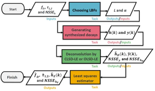
3. Theoretical simulations & analysis of realistic FLIM data (GNRs in Hek293 cells) Figure 1 shows the flow diagram summarizing how the performances of OLSD-LE and CLSD-LE on bi-exponential decays (0 < fD < 1, 0.1ns ≤τ1≤ 0.9ns and 2ns ≤τ2≤ 3ns) were

assessed in four steps, highlighted in different colours. The flow diagram can also be applicable to realistic FLIM data by replacing the synthesized data with the measured data.

Fig. 1. Flow diagram for testing LSD-LE on bi-exponential decays.

3.1 Symthesized FLIM data analysis

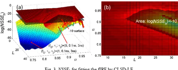
Firstly, LBFs were chosen to ensure that a given NSSEh, Eq. (5), can be met. We set log(NSSEh) < −10 (natural logarithm), and NSSEh was computed for two extreme cases (fD = 0, τ1 = 0.1ns, τ2 = 3ns) and (fD = 1, τ1 = 0.1ns, τ2 = 3ns) as a function of L and α. Figures 2 and

3 show the NSSEh plots for OLSD-LE and CLSD-LE, respectively. The shadowed areas shown in Figs. 2(b) and 3(b) are where L and α should be selected to meet log(NSSEh) < −10, and all other combinations (0.1ns ≤τ1≤ 0.9ns and 2ns ≤τ2≤ 3ns) surely meet this condition.

To reduce instability (ill-conditioned VT_{V deteriorates stability), computation and overfitting}

(for OLSD-LE), the smallest L within the shadowed area is suggested. Therefore, Fig. 2(b) shows that the optimal LBFs for OLSD-LE has L = 12 and α = 0.924, whereas Fig. 3(b) suggests L = 16 and α = 0.912 for CLSD-LE. Obviously CLSD-LE needs a larger L and is slightly more complicated computationally.

Fig. 3. NSSEh for fitting the fIRF by CLSD-LE.

In general, LSD-LE methods need to specify L and α properly for robust analysis. Usually the lifetime range in the field of view can be known before experiments; this information can be used to obtain new residual plots similar to Figs. 2 and 3. For a given residual requirement,

L is suggested to be as small as possible to ensure a faster analysis speed. On the other hand, to improve the resolvability for the smaller lifetime τ1, it is required that L cannot be too

small. The selection of L is a trade-off between the speed and the lifetime resolvability, whereas α determines the accuracy of the fitting. For these reasons L = 16 and α = 0.912 and

L = 12 and α = 0.924 are chosen for CLSD-LE and OLSD-LE, respectively.

Secondly, the synthesized decays, y(k), were generated according to the paramters listed in Table 1. There are nine different h(k), with (fD, τ1) = (0.8, 0.2ns), (0.8, 0.5ns), (0.8, 0.8ns), …,

and (0.2, 0.8ns) respectively, generated from Eq. (3), and nine corresponding y(k) (k = 1,2,…,9) were generated from Eq. (2).

Table 1. Settings for the parameters

fD τ1 (ns) τ2 (ns) FWHM of iIRF (ns) T (ns) N

0.8, 0.5, 0.2 0.2, 0.5, 0.8

2.5 0.3 10 256

Thirdly, CLSD-LE (L = 16, α = 0.912), OLSD-LE (L = 12, α = 0.924 and L = 16, α = 0.912) were applied to y(k) to obtain the recovered fIRF, ĥD(k), and NSSEy and NSSEhD were used to assess the performances as shown in Fig. 4 where axis x corresponds to k in y(k). Being different from the previous analysis in Fig. 3 where Poisson noise was not included. This analysis shows how a larger L is more likely to cause overfitting after Poisson noise sources are included. In this analysis, 500 Monte Carlo simulations were performed for each

y(k). Because of overfitting, µNSSE,y for OLSD-LE (L = 16) is larger than µNSSE,y for OLSD-LE (L = 12). Although µNSSE,y for OLSD-LE (L = 12) is almost equal to that for CLSD-LE,

µNSSE,hD of OLSD-LE is in general larger than that of CLSD-LE, showing that CLSD-LE performs better and produces a ĥD(k) closer to h(k).

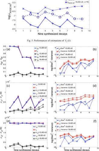
Finally, LSE is applied to ĥD(k) to obtain fD̂ and τˆ1,2. Figure 5 shows NSSEhE for CLSD-LE and OLSD-CLSD-LE. Again, µNSSE,hE for CLSD-LE is smaller than that for OLSD-LE. It shows that all ĥE(k) obtained by CLSD-LE are closer to h(k), giving much better estimations.

Fig. 5. Performances of estimations of h kˆ ( )_E

Figure 6 shows the performances of the estimated f̂D and τˆ1,2. All µx (x = f̂D or τˆ1,2) obtained by OLSD-LE and CLSD-LE are close to xr and all Variance are bigger than the corresponding Bias2_{, suggesting that both methods are effective. And σ}

x and Variance for CLSD-LE are smaller than those for OLSD-LE, indicating that CLSD-LE is more robust against the noise. Figure 6 shows the performances of f̂D and τˆ1,2: (a) and (b) for fD, (c) and (d) for τ1, and (e) and (f) for τ2. Figures 6(a), 6(c), and 6(e) show that with a fixed fD a larger τ1

gives less precise estimations, and with a fixed τ1 a reduced fD gives less precise τ1 but more

precise τ2. These trends are reasonable. Figures 6(b), 6(d), and 6(f) show that although

OLSD-LE produces less biased results and each case is Variance-limited, CLSD-LE produces smaller variances and therefore performs better in all cases.

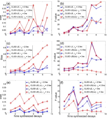
Fig. 7. Bias performances (a) ΔfD/fD, (c) Δτ1/τ1, and (e) Δτ2/τ2 and F-value (b) F(fD), (d) F(τ1),

and (f) F(τ2) of the proposed and Liu’s CLSD-LE for T/τ2 = 4 or 3.3.

of x (x = fD, τ1, or τ2), NC is the photon count; it is used to characterize the photon efficiency of an algorithm [37]) and the bias (Δx/x) using Liu’s CLSD-LE and our CLSD-LE. Figures 7(b), 7(d) and 7(f) shows that our CLD-LE has comparable or better F-value performances than Liu’s CLSD-LE for τ2 = 2.5 (T/τ2 = 4). However, Figs. 7(a), 7(c) and 7(e) shows our

CLSD-LE has superior bias performances. Liu’s CLSD-CLSD-LE needs to meet the requirement that the LBFs should be orthonormal and therefore the largest α they can use is 0.877 when L = 16 (in order to compare with our method). A lower α usually contributes a larger bias. To demonstrate how the ratio T/τ2 affects Liu’s CLSD-LE, we reduced T/τ2 to 3.3 by setting τ2 =

3ns. Figure 7 shows that Liu’s CLSD-LE has worse bias performances in all parameters, whereas the proposed CLSD-LE has similar bias performances as the previous example (T/τ2

= 4). The F-value of Liu’s method seems smaller for τ1 and τ2, but this should not be misled to

conclude that its photon efficiency is better [38]. Instead, it is due to the seriously biased estimations [38]. Compared with Liu’s approach, the proposed CLSD-LE performs more consistently.

3.2 Real FLIM data analysis

The proposed method was also tested on two-photon FLIM images of Cy5-ssDNA-GNRs labelled Hek293 cells. The images are for evaluating the endocytosis of gold nanorods (GNR) in living cells. The detailed synthesis of GNR-based RNA nanoprobes can be found elsewhere [39]. In brief, GNRs were functionalized with thiolated oligonucleotides (ssDNA) labeled with Cy5 through ligand exchange and salting aging process. After the incubation with Cy5-ssDNA-GNRs, Hek293 cells were washed and fixed with paraformaldehyde. Two-photon FLIM experiments were performed on an LSM 510 confocal microscope (Carl Zeiss) using the SPC-830 TCSPC acquisition system (Becker & Hickl GmbH). A Ti:sapphire laser (Chameleon, Coherent) was used (at 800 nm) to generate laser pulses with a duration less than 200 fs. The timing resolution of the TCSPC is 0.039ns, and measured histograms with 256 time bins (T = 256 × 0.039 = 10ns) were recorded.

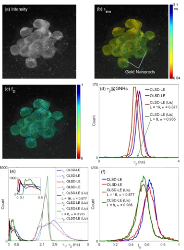
Figure 8(a) shows the gray-scale intensity image of Hek293 cells. Figures 8(b) and 8(c) show the average lifetime, τave = fDτ1 + (1–fD)τ2, and fD images, respectively, obtained by the proposed CLSD-LE (L = 16, α = 0.912), where τ1 is the lifetime of GNRs (usually less than

100ps [39]) and τ2 is the fluorescence lifetime of Cy5. Figures 8(a) and 8(b) demonstrate the

superiority of FLIM imaging over intensity imaging in identifying the locations of GNRs. Figures 8(b) and 8(c) show that the fluorescence of Cy5 was largely quenched by GNRs due to the fluorescence energy transfer (FRET) arising from the hairpin structure of ssDNA [39]. Hybridization of nanoprobes with target RNA in cells opens the hairpin structure and results in significant increase in fluorescence intensity (the fD map can help locate GNRs; fD > 0.8 &

τ1 < 100ps) and decrease in τ2. In the areas where the energy transfer appears, the fluorescence

Fig. 8. (a) Intensity, (b) τave, and (c) fD maps and (d) τ2 histograms at GNRs, (e) lifetime

histograms, and (f) fD histograms of Hek293 cells.

Figure 8(d) shows the τ2 histogram at GNRs (fD > 0.8 & τ1 < 100ps), and it shows a

reduced τ2 around 2.1ns and 2.0ns for the proposed CLSD-LE (L = 16, α = 0.912) and

OLSD-LE (L = 12, α = 0.924), respectively. In order to show the advantages of the proposed CLSD-LE, different CLSD-LE approaches were applied to the analysis. Figure 8(e) shows τ1 and τ2

in the figure shows τ1 histograms within (0, 0.5ns), and it explains why a larger L is required

for resolving the lifetimes of GNRs (τ1 < 100ps). The discrepancy in τ2 histograms between

the proposed and the Liu’s CLSD-LE is due to the fact that a large number of pixels show no energy transfer and contain a larger τ2 around 3ns. For Liu’s CLSD-LE, the lower T/τ2 (~3)

limits its resolvability for τ2 (unable to resolve τ2 > 3ns) causing misinterpretation that there is

energy transfer at these pixels. This observation is in good agreement with Fig. 7(e), T/τ2 =

3.3. In Fig. 8(d), there is a population of pixels showing τ1 < 100ps, indicating that there is

energy transfer between GNRs and Cy5. For Liu’s CLSD-LE, however, a smaller L (L = 8) results in biased estimations of τ1, not able to allocate GNRs (green curve). The maximum α

can be applied is 0.877 (for L = 16) for Liu’s CLSD-LE to meet the orthonormality requirement (note that it is only quasi-orthonormal). This lower α leads to a bigger bias in τ2.

For our methods, although there is a slight discrepancy between CLSD-LE and OLSD-LE, they are still be able to provide similar contrast. Compared with our previous report [37], the results show that considering the iIRF in the analysis would improve locating GNRs. The results also show that the proposed CLSD-LE and OLSD-LE produce similar results, and both work robustly even when the ratio T/τ2 is less than 4. Unlike previously reported LSD-LE

[22–29] and BCMM [37] requiring a much larger T/τ2 or extra bias correction procedures (for

BCMM), the proposed method can reduce the acquisition time per measurement. Figure 8(f) also shows that our CLSD-LE and OLSD-LE produce similar fD histograms, whereas for Liu’s CLSD-LE a smaller T/τ2 causes biased fD estimations, see Fig. 7(a). The analysis results show that the proposed OLSD-LE and CLSD-LE are effective and have potential to be used to analyze FLIM-FRET data, with the latter showing better performances.

4. Conclusion

We presented new criteria to choose LBFs for LSD-LE based only on how close the Laguerre expansion can approximate the fIRF. Different from the conclusion suggested by previous studies, the proposed criteria do not need to consider the mutual orthonormalities between LBFs. The new criteria do not require that the LBFs and the corresponding derivatives to be close to zero at the end of the measurement window, and they allow using a smaller T/τ2 ratio

and therefore reducing the acquisition time per measurement. We applied this upgraded method to analyzing bi-exponential decays and its performances (on both CLSD-LE and OLSD-LE) were accessed and compared against the original CLSD-LE. The results show that both the upgraded CLSD-LE and OLSD-LE can be applicable to our studies, but the former performs slightly better. Both synthesized and realistic experimental FLIM data show that the proposed CLSD-LE has better performance than the original CLSD-LE when T/τ2 is small

and suggest that the proposed CLSD-LE can be an effective tool to analyze bi-exponential FLIM-FRET data. It can be further extended to study multi-exponential decays in the future. The proposed methods should be able to encourage wider applications of fast FLIM technologies and gold nanoparticles for cancer therapy [37, 39–41].

Acknowledgments