City, University of London Institutional Repository
Citation
:
Jones, P. R. ORCID: 0000-0001-7672-8397 (2016). A note on detecting
statistical outliers in psychophysical data (10.1101/074591). .
This is the draft version of the paper.
This version of the publication may differ from the final published
version.
Permanent repository link:
http://openaccess.city.ac.uk/20361/
Link to published version
:
http://dx.doi.org/10.1101/074591
Copyright and reuse:
City Research Online aims to make research
outputs of City, University of London available to a wider audience.
Copyright and Moral Rights remain with the author(s) and/or copyright
holders. URLs from City Research Online may be freely distributed and
linked to.
City Research Online:
http://openaccess.city.ac.uk/
[email protected]
Detecting statistical outliers in
psychophysical data
1
Pete R. Jones1,2 2
1Institute of Ophthalmology, University College London (UCL), UK, EC1V 9EL 2NIHR Moorfields Biomedical Research Centre, London, UK, EC1V 2PD
3
4
Abstract: This paper considers how best to identify statistical outliers when the underlying sampling distribution is unknown. Eight methods are described, and each is evaluated using Monte Carlo simulations of a typical psychophysical experiment. The best method is shown to be one based on a measure of absolute-deviation known asSn. In particular, this method is shown to be more accurate than popular heuristics based on standard deviations from the mean, and more robust than non-parametric methods based on interquartile range.
5
PACS numbers:43.66.Yw 6
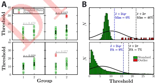
1. The problem of outliers 7
A statistical outlier is an observation that diverges abnormally from the overall pattern
8
of data. They are often generated by a process qualitatively distinct from the main
9
body of data. For example, in psychophysics, spurious data can be caused by technical
10
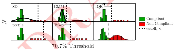
error, faulty transcription, or — perhaps most commonly — participants being unable
11
or unwilling to perform the task in the manner intended (e.g., due to boredom,
12
fatigue, poor instruction, or malingering). Whatever the cause, statistical outliers can
13
profoundly affect the results of an experiment1, making similar populations appear
14
distinct (Fig 1A, top panel), or distinct populations appear similar (Fig 1A, bottom 15
panel). For example, it is tempting to wonder how many ‘developmental’ differences
16
between children and adults are due to a small subset of non-compliant children.
17
1 2
p= 0.2 7 7
1 2
0 10 20 30 40
p= 0.0 0 8
Group
T
h
r
e
s
h
o
ld
0 10 20 30 40
p= 0.4 7 2
p= 0.0 4 5
Sta nda rd Da ta O utlier
T
h
r
e
s
h
o
ld
¯
x+ 2σ
FA = 7%
˜
x+ 2iqr
FA = 9%
0 5 10 15 20 25 30 ¯
x+ 2σ
FA = 7%
˜
x+ 2iqr
FA = 9%
Threshold
N StandardOutlier ¯
x+ 2σ
Miss = 46%
˜
x+ 2iqr
Miss = 0% ¯
x+ 2σ
Miss = 46%
˜
x+ 2iqr
Miss = 0%
N
A
B
Fig1. Examples of (A) how the presence outliers can qualitatively affect the overall
pattern of results, and (B) common errors made by existing methods of outlier
identification heuristics.P-values pertain to the results of between-subjectt-tests.
See body text for details.
[image:2.612.166.431.501.643.2]2. General approaches and outstanding questions 18
One way to militate against outliers is to only ever use non-parametric statistics (i.e.,
19
which have a high breakdown point2, and so tend to be robust against extreme
20
values). In reality though, this approach often proves impractical, since non-parametric
21
methods are less powerful, less well understood, and less widely available than
22
their parametric counterparts. Alternatively, some experimenters identify and remove
23
outliers ‘manually’, using some unspecified process of ‘inspection’. This approach is
24
not without merit. However, when used in isolation, manual inspection is susceptible
25
to bias and human error, and it precludes rigorous replication or review. Finally then,
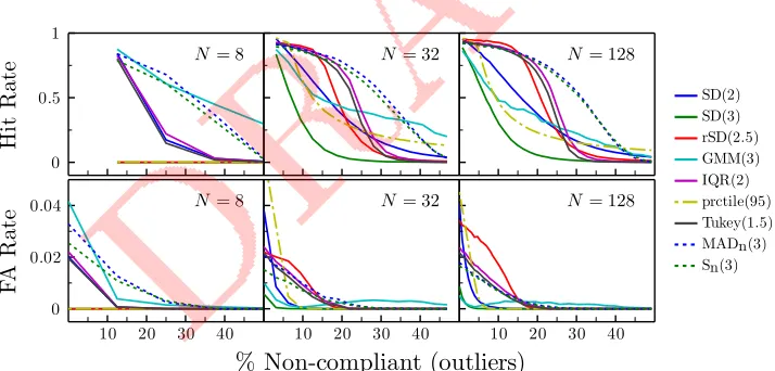
26
statistical outliers can be identified numerically. If the underlying sampling distribution
27
is known, then it is trivial to set a cutoff based on the likelihood of observing a given
28
data point. However, when the sampling distribution is unknown, researchers are
29
often compelled to use numerical heuristics, such as “was the data point more thanN
30
standard deviations from the mean?”. Currently, however, a plethora of such heuristics
31
exist. It is unclear which method works best, and at present unscrupulous individuals
32
are free to pick-and-choose whichever yields the outcome they expect/desire. The
33
goal of this work was therefore(i)to describe what methods are currently available
34
for identifying statistical outliers (in datasets generated from an unknown sampling
35
distribution), and(ii)to use simulations to assess how well each method performs in
36
a typical psychophysical context.
37
3. State-of-the-art methods for identifying statistical outliers 38
Here we describe eight methods for identifying statistical outliers. Five of these
39
methods are also shown graphically in Fig 2.
40
SD xi=outlier if it lies more thanλstandard deviations,σ, from the mean,x¯:
41
|xi|>(¯x+λσ), (Eq 1)
whereλis typically between 2 (liberal) and 3 (conservative). This is one of the most
42
commonly used heuristics, but is theoretically flawed. Both the¯xandσterms are easily
43
distorted by extreme values, meaning that more distant outliers may ‘mask’ lesser ones.
44
This can lead to false negatives (identifying outliers as genuine data; Fig 1B,top panel).
45
The method also assumes symmetry (i.e., attributes equal importance to positive and
46
negative deviations from the center), whereas psychometric data are often skewed.
47
This can lead to false positives (identifying genuine data as outliers; Fig 1B,bottom 48
panel). Furthermore, whileSDdoes not explicitly require normality, the±λσ bracket
49
may include more or less data than expected if the data are not Gaussian distributed.
50
For example,±2σincludes 95% of data when Gaussian distributed, but as little as 75%
51
otherwise (Chebyshev’s inequality).
52
GMM xi=outlier if it lies more than λ standard deviations from the mean of the
53
primary component of a Gaussian Mixture Model:
54
|xi|>(¯x1+λσ1) where pdf(x) =ωΦ(x;µ1, σ1) + (1−ω)Φ(x;µ2, σ2). (Eq 2)
An obvious extension toSD: The two methods are identical, except that when fitting
55
the parameters to the data, the GMM model also includes a secondary component
56
designed to capture any outliers (see Fig 2). The secondary component is not used to
57
identify outliers per se, but prevents extreme values from distorting the parameters
58
of the primary component. In practice the fit of the secondary component must be
59
constrained to prevent it ‘absorbing’ non-outlying points (seeSupplemental Material).
60
rSD Same asSD, but applied recursively until no additional outliers are identified:
61
(
|x0i|>(¯x0+λσ0) |xn
i|>(¯xn+λσn).
(Eq 3)
This approach aims to solve the problem of masking by progressively peeling away
62
the most extreme outliers. However, like SD, it remains intolerant to non-Gaussian
63
distributions. In situations where samples are sparse/skewed, this approach therefore
64
risks aggressively rejecting large quantities of genuine data (see Fig 1B). Users typically
65
attempt to compensate for this by using a relatively high criterion level, and/or by
66
limiting the number of recursions (e.g.,λ≥3, nmax= 3).
67
IQR xi=outlier if it lies more thanλtimes the interquartile range from the median:
68
|xi|>(˜x+λiqr). (Eq 4) This is a non-parametric analog of theSDrule: substituting median andiqr for mean
69
and standard deviation. Unlike SD, the key statistics are relatively robust. Thus, the
70
breakdown points forx˜andiqrare 50% and 25% (respectively), meaning that outliers
71
can constitute up to 25% of the data before the statistics start to be distorted3.
72
However, likeSD, theIQRmethod only considers absolute deviation from the center. It
73
is therefore insensitive to any asymmetry in the sampling distribution (Fig 1B,bottom).
74
prctile xi=outlier if it lies above theλthpercentile, or below the(1−λ)th:
75
xi> Pλ or xi < P1−λ. (Eq 5) This effectively ‘trims’ the data, rejecting the most extreme points, irrespective of their
76
values. UnlikeIQR, this method is sensitive to asymmetry in the sampling distribution.
77
But it is otherwise crude in that it ignores any information contained in the spread of
78
the data points. The prctile method also begs the question in that the experimenter
79
must estimate, a priori, the number of outliers that will be observed. If λ is set
80
incorrectly, genuine data will be excluded, or outliers missed.
81
Tukey xi=outlier if it lies more thanλtimes the iqr from the 25th/75thpercentile:
82
xi>(P75+λiqr) or xi<(P25−λiqr). (Eq 6)
Popularized by John W. Tukey, this attempts to combine the best features of theIQRand
83
prctilemethod. The information contained in the spread of data,iqr, is combined with
84
the use of lower/upper quartile ‘fences’ that provide some sensitivity to asymmetry.
85
MADn xi=outlier if it lies farther from the median thanλtimes the median absolute
86
distance [MAD] of every point from the median:
87
|x
i−x˜|
M ADn
> λ where M ADn= 1.4826 med
i=1:n|xi−jmed=1:nxj|, (Eq 7) where 1.4826 is simply a scaling factor, used for consistency with the standard
88
deviation over a Gaussian distribution (see Ref [3]). Unlike the non-parametric
89
methods described previously, this method uses MAD rather thaniqras the measure of
90
spread. This makes this method more robust, as the MAD statistic has the best possible
91
breakdown point (50%, versus 25% foriqr). However, as with IQR, MADn assumes
92
symmetry, only considering the absolute deviation of datapoints from the center.
93
Sn xi=outlier if the median distance of xi from all other points, is greater thanλ
94
times the median distance of every point from every other point:
95
med
j6=i|xi−xj|
Sn
> λ where Sn= 1.1926cnmed i=1:n
med
j6=i |xi−xj|
, (Eq 8)
where 1.1926 is again for consistency with the standard deviation, andcn is a finite
96
population correction parameter (see Ref [3]). Like MAD, the Sn term is maximally
97
robust. However, this method differs from MADn in that Sn considers the typical
98
distance between all data points, rather than measuring how far each point is from a
99
central value. It therefore remains valid even if the sampling distribution is asymmetric.
100
The historic difficulty with Sn is its long computational time [O(n2)]. However, for
101
psychophysical applications this is trivial given modern computing.
102
4. Comparison of techniques using simulated psychophysical observers 103
To assess the eight methods described in Section 3, we applied each to random
104
samples of data prelabeled as either ‘good’ or ‘bad’. However, rather than simply
105
specifying arbitrary sampling distributions for each of these categories, we generated
106
data by simulating a typical two-alternative forced-choice [2AFC] experiment in which
107
a 2-down 1-up transformed staircase4 was applied to N simulated observers. Each
108
observer consisted essentially of a randomly generated psychometric function, and
109
made stochastic, trial-by-trial responses based on the current stimulus level and a
110
random sample of additive internal noise (i.e., the variance of which was determined
111
by the slope of their psychometric function). Trial-by-trial response data were then
112
processed and analyzed as if from human participants, leading, for example, to the
113
sampling-distributions of 70.7% thresholds shown in Fig 2 (bottom right).
114
Of the N observers, X% were ‘non-compliant’ (on average, their psychometric
115
functions had a higher mean, standard deviation, and lapse-rate), and were thus
116
likely to produce outlying data points (Fig 2,red bars). The remaining observers were
117
‘compliant’ (on average lower mean, standard deviation, and lapse-rate), and produced
118
the distribution of ‘good’ data shown in green. Precise details of all test parameters can
119
be found in theSupplemental Material, which contains the complete MATLABcode used 120
to generate all of the data presented here.N took the valuesh8,32,128i, representing
121
small, medium, and large sample sizes, while the number of non-compliant observers
122
varied from 0 to 50% ofN (e.g.,h0,1, ...,16i, when whenN=32). For each condition,
123
2,000independent simulations were run, for a total of 108K simulations.
124
SD GMM IQR
prctile Tukey
70.7% Threshold
N
Compliant Non-Compliant
cutoff,κ
Fig2. Simulation methods. Random sample of thresholds were generated, of which
X%came from ‘non-compliant’ simulated observers (here:N=32,X%=19). Each
of eight methods were then used to identify which observations were generated by ‘non-compliant’ observers (i.e., likely statistical outliers). Only five methods are
depicted here, as the other three (rSD,MADn andSn) have no obvious graphical
analog. The final panel shows the full sampling distributions over 20,000 trials, and the ideal unbiased classifier, for which: Hit rate = 0.97, False Alarm = 0.05.
Results and Discussion
125
The results are shown in Fig 3. We begin by considering only the case where N=32 126
(Fig 3,middle column), before considering the effect of sample size.
127
As expected, the SD rule proved poor. When λ=3, it was excessively conservative –
128
seldom exhibiting false alarms, but missing the great majority of outliers, particularly
129
[image:5.612.123.472.443.543.2]as the number of outliers increased. Lowering the criterion to λ=2 yielded more
130
reasonable results. However, SD still exhibited a lower hit rate than most other
131
methods, and also exhibited a high false alarm rate when there were few/no outliers.
132
The modified GMM and rSD rules exhibited increased robustness and accuracy,
133
respectively. However, compared to non-parametric methods, they were generally only
134
more sensitive than theprctilemethod, which was only accurate when the predefined
135
exclusion rate matched the true number of outliers exactly.
136
The two iqr-based methods, IQR and Tukey, exhibited high sensitivity when the
137
number of outliers was low (≤20%). However, as expected, they exhibited a marked
138
deterioration in hit rates when the number of outliers increased beyond 20% (i.e., in
139
accordance with the 25% breakdown point foriqr).
140
The two median-absolute-deviation-based methods,MADn andSn, were as sensitive
141
as all other methods when outliers were few (≤20%), and were more robust than
142
theiqrmethods – continuing to exhibit high hit rates and few false alarms even when
143
faced with large numbers of outliers. Compared to each other,MADnandSnperformed
144
similarly. However, the Snstatistic makes no assumption of symmetry, and so ought to 145
be superior in situations where the sampling distribution is heavily skewed.
146
We turn now to how sample size affected performance. With large samples (N=128),
147
the pattern was largely unchanged from the medium sample-size case (N=32), except
148
thatrSDexhibited a marked increase in false alarms, making it an unappealing option.
149
With small samples (N=8), theprctileandrSDmethods became uniformly inoperable,
150
while most other methods were unable to identify more than a single outlier. TheMADn
151
andSn methods, however, remained relatively robust, and generally performed well,
152
though they did exhibit an elevated false alarm rate when there were few/no outliers.
153
It may be that this could be rectified by increasing the criterion,λ, as a function ofN,
154
however this was not investigated here. TheGMMmethod also performed well overall
155
in the small-sample condition. However, it did also exhibit the highest false alarm rate
156
when there were no outliers, and was only more sensitive thanMADnorSn when the
157
proportion of outliers was extremely high (>33%).
158
Hi
t
R
at
e
F
A
R
at
e
% Non-compliant (outliers)
0 0.5 1
N= 8 N= 32 N= 128
10 20 30 40 0
0.02
0.04 N= 8
10 20 30 40
N= 32
10 20 30 40
N= 128
SD(2) SD(3) rSD(2.5) GMM(3) IQR(2) prctile(95) Tukey(1.5) MADn(3) Sn(3)
Fig3. Simulation results. The eight classifiers described inSection 3were used to
distinguish between random samples of ‘compliant’ and ’non-compliant’ simulated
observers (see Fig 2). Numbers in parentheses indicate the criterion level,λ, used
by each classifier.
[image:6.612.121.478.431.602.2]5. Summary and concluding remarks 159
Of the eight methods considered, Sn proved the most sensitive and robust. Specific 160
situations were observed in which other heuristics performed as-well-as or even better
161
thanSn: for example, when the sample size was large (rSD), or when the proportion 162
of outliers was very low (IQR,Tukey) or very high (GMM). However, most methods
163
were less sensitive in than Sn in the majority circumstances, and failed precipitously
164
in some circumstances, making them unattractive alternatives. The related method
165
MADnalso proved strong, and could be considered a viable alternative toSn. However, 166
as discussed in Section 3, MADn assumes a symmetric sampling distribution, and so
167
would not be expected to perform as well if the sampling distribution was very heavily
168
skewed (e.g., when dealing with reaction time data). The popularSD metric proved
169
particularly poor in all circumstances, and should never be used. In short,Snappears to
170
provide the best means of identifying statistical outliers when the underlying sampling
171
distribution is unknown. Its use may be particularly beneficial for researchers working
172
with small/irregular populations such as children, animals, or clinical cohorts. MATLAB 173
code for computingSnis provided in theSupplemental Material. 174
Limitations of the present study
175
The present findings are predicated on finite simulations of a single experimental
176
paradigm, and so cannot be guaranteed to generalize. Anecdotally, the same overall
177
pattern of results remained unchanged when key parameters were varied (e.g.,
178
properties of the observers and/or of the experimental paradigm). However, there
179
exist an infinite number of possible circumstances, and some experimental paradigms
180
— particularly those involving advanced adaptive procedures — are capable of
181
producing quite complex (e.g., bimodal) sampling distributions. With this in mind,
182
the code in Supplemental Material also provides support for a variety of paradigms
183
(transformed/weighted staircases, Constant Stimuli, and various more advanced
184
procedures, implemented via the Palamedes toolbox5). Readers are encouraged to
185
simulate their own experimental configurations, to assess how each method performs.
186
On the ethics of excluding statistical outliers
187
Excluding outliers is often regarded as poor practice. As shown inSection 1, however,
188
the exclusion of outliers can sometimes be preferable to reporting misleading results.
189
Automated methods of statistical outlier identification should never be used blindly
190
though, and they are not a replacement for common sense. Where feasible, datapoints
191
identified as statistical outliers should only be excluded in the presence of independent
192
corroboration (e.g., experimenter observation). Furthermore, best practice dictates
193
that when outliers are excluded, they should continue to be shown graphically, and
194
all statistical analyses should be run twice: with and without outliers included.
195
Acknowledgments 196
This work was supported by the NIHR Biomedical Research Centre located at (both)
197
Moorfields Eye Hospital and the UCL Institute of Ophthalmology.
198
References 199
[1] Osborne, J. W. & Overbay, A. The power of outliers (and why researchers should always check for them). 200
Practical assessment, research & evaluation9, 1–12 (2004). 201
[2] Huber, P. J.International Encyclopedia of Statistical Science, chap. Robust Statistics, 1248–1251 (Springer 202
Berlin Heidelberg, Berlin, Heidelberg, 2011). 203
[3] Rousseeuw, P. J. & Croux, C. Alternatives to the median absolute deviation. Journal of the American
204
Statistical association88, 1273–1283 (1993). 205
[4] Levitt, H. Transformed up-down methods in psychoacoustics. The Journal of the Acoustical Society of
206
America49, 467–477 (1971). 207
[5] Kingdom, F. & Prins, N.Psychophysics: a practical introduction(Elsevier Academic Press, 2010), 1 edn. 208