City, University of London Institutional Repository
Citation: Meulemans, W. & Haunert, J-H. (2016). Partitioning Polygons via Graph
Augmentation. Lecture Notes in Computer Science, 9927, pp. 18-33. doi:
10.1007/978-3-319-45738-3
This is the accepted version of the paper.
This version of the publication may differ from the final published
version.
Permanent repository link: http://openaccess.city.ac.uk/15169/
Link to published version: http://dx.doi.org/10.1007/978-3-319-45738-3
Copyright and reuse: City Research Online aims to make research
outputs of City, University of London available to a wider audience.
Copyright and Moral Rights remain with the author(s) and/or copyright
holders. URLs from City Research Online may be freely distributed and
linked to.
Partitioning Polygons via Graph Augmentation
Jan-Henrik Haunert1,? and Wouter Meulemans2
1
Institute of Computer Science, University of Osnabr¨uck, Germany.
2
giCentre, City University London, United Kingdom.
Abstract. We study graph augmentation under the dilation criterion. In our case, we consider a plane geometric graphG= (V, E) and a setC
of edges. We aim to add toGa minimal number of nonintersecting edges fromCto bound the ratio between the graph-based distance and the Eu-clidean distance for all pairs of vertices described byC. Motivated by the problem of decomposing a polygon into natural subregions, we present an optimal linear-time algorithm for the case that P is a simple poly-gon andC models an internal triangulation ofP. The algorithm admits some straightforward extensions. Most importantly, in pseudopolynomial time, it can approximate a solution of minimum total length or, ifC is weighted, compute a solution of minimum total weight. We show that minimizing the total length or the total weight is weakly NP-hard. Finally, we show how our algorithm can be used for two well-known problems in GIS: generating variable-scale maps and area aggregation.
1
Introduction
Polygons representing geographic objects can contain millions of vertices and thus can be difficult to handle. Often, they consist of multiple regions that are connected only via narrow bottlenecks, such as isthmuses in the case of land or straits in the case of water areas. To ease the handling of such polygons and to identify natural subregions, such as the Iberian Peninsula as a part of Europe, one often seeks a partition of a polygon into multiple smaller polygons of a certain type (e.g., into convex polygons). A triangulation of a polygon is the most common type of a polygon partition, yet often one is interested in larger (non-triangular) subregions. We present new algorithms for partitioning a polygon based on an internal triangulation of it: every output region is the union of a set of triangles of that triangulation. We consider our algorithm a useful tool for shape manipulation and demonstrate its effectiveness on two use cases: the generation of variable-scale maps and the aggregation of areas.
Our basic idea is to consider the polygon partitioning problem as a special graph augmentation problem. The vertices and edges of the input polygon P define a geometric graphG, which we augment with a selection of edges from a setCof candidate edges (that is, diagonals ofP) to splitP into multiple pieces.
?
After the augmentation, the graph shall be well connected. More precisely, for each candidate edge {u, v} ∈ C we require that the dilation for u and v in the augmented graph is bounded by a user-set parameter. For any two vertices u, v of a geometric graphG, the dilation (sometimes also called stretch factor or detour factor) is defined as the ratio between the shortestu-vpath viaGand the Euclidean distance betweenuand v. By selecting a minimum number of edges from Cwe obtain a nice decomposition of the input polygon. As an alternative optimization objective we consider minimizing the total weight of the selected edges, assuming that for each edge in Ca weight is given as part of the input.
Contributions. We introduce terminology and a general problem definition with three primary variants (unweighted, length-weighted and general weights) in Section 2. We review related work in Section 3. In Section 4 we consider the problem variants for the case that the graph to be augmented is a simple polygon without holes and the edges that can be added are an internal triangulation. We provide an optimal linear-time algorithm for the unweighted case, and present some extensions. We prove that both the general-weights case and the length-weighted case are weakly NP-hard, present a pseudopolynomial-time algorithm for the general-weights case, and show that it can provide a (1+ε)-approximation algorithm for the length-weighted case. We discuss our two use cases in Section 5.
2
Preliminaries
Graphs. Let G = (V, E) denote a graph defined by its vertices V and edges E⊆ {{u, v} |u, v∈V}. We callGageometric graph if every vertex is assigned a position inR2and each edge is represented by the line segment connecting its endpoints. A geometric graph is plane if vertices have unique positions and no two edges intersect, except at common endpoints.
Dilation. LetG= (V, E) be a geometric graph andu, v∈V be two vertices of G. We denote the Euclidean distance between uand v as ku−vk; we use kek
to denote the length of edge e. The length of the shortest path in G between uand v is denoted by dG(u, v). We define the (vertex) dilation betweenuand
v as ∆G(u, v) = dG(u, v)/ku−vk; the dilation of the entire graph is ∆G =
maxu,v∈V,u6=v∆G(u, v). IfGis disconnected, its dilation is infinite.
Problem statement.In this paper, we consider graph augmentation problems, where the augmentation is constrained to a prescribed set of vertex pairs. We call such vertex pairscandidate edges. Hence, aproblem instance comprises
– a plane geometric graphG= (V, E),
– a setC⊆ {{u, v} |u, v∈V}\E of candidate edges, and
– a real numberτ≥1.
ConsiderS ⊆C to be a subset of the candidate edges. We denote byGS =
simple path inGS whose length is sufficiently small to prove that∆GS(u, v)≤τ
is called a witness of {u, v}. Set S is a solution to the problem if all edges in C are satisfied (with respect to S). Note that we ask to satisfy only the pairs specified by the candidate edges; we do not guarantee that the dilation between all vertices is bounded byτ. This is a trade-off that we make to guarantee that solutions exist. In particular,S=C is a solution for any problem instance.
However, we want to find a “good” solution. A primary criterion, in the context of polygon partitioning, is that the edges in S do not intersect each other or existing edges ofG. Furthermore, we consider optimizing three different objective functions, resulting in the following problems:
– MinSize: minimize|S|.
– MinLength: minimizeP
e∈Skek.
– MinWeight: minimizePe∈Sw(e), given weightsw:C→R+.
In the above, we provide an upper bound on the allowed dilation and mini-mize the cost (size, length or weight) of the solution. The dual variants instead bound the allowed cost and ask to minimize the dilation. We focus on the stated variants; our algorithms can solve the dual variant by a binary search onτ. This is possible since the problem is monotonic: any solution forτ is also a solution forτ0 > τ, and thus increasing the dilation can only reduce the minimal cost.
3
Related Work
Partitioning.Partitions of polygons into triangles, monotone polygons, or con-vex polygons are common in the context of GIS [19] and have intensively been studied in computational geometry. For example, for the case that no additional vertices (i.e.,Steiner points) are allowed, Keil and Snoeying [13] have shown that a simple polygon withn vertices andr reflex vertices can be partitioned into a minimum number of convex polygons inO(n+r2min{r2, n}) time. In the case that Steiner points are allowed, the problem can be solved inO(n+r3) time [5]. For polygons with holes, the problem is NP-hard in both cases [16].
Often motivated by problems in computer vision and pattern recognition, researchers have developed methods for partitioning polygons into “natural and intuitive” [17], “simpler” [8], or “approximately convex” [15] pieces, which need not be convex. However, these methods do not provide any guarantee of opti-mality with respect to the number of output pieces or a different measure.
Dilation. Algorithmic work involving dilation is motivated mostly by applica-tions in infrastructure design (e.g. road or electricity networks). Much research has been done without planar considerations, e.g. [2]. Considering our use cases, we focus here on results with such planar considerations; see [4] for a survey.
Giannopoulos et al.[9] prove that, given a point setQ, computing a graph G = (Q, E) with ∆G ≤ 7 is NP-hard, if |E| is bounded toO(|Q|). They also
the investigation of our variant, where we do not consider satisfying all pairs, but only those provided in a (constrained) candidate set.
Farshi et al. [7] show that it is possible to compute, for a given geometric graph, the edge that results in the largest dilation reduction inO(n4) time. This was later improved by Wulff-Nilsen [20] toO(n3logn) time. Note that repeatedly applying this greedy choice does not yield an optimal result. Aronov et al. [1] present algorithms for the following problem: given a point inside a polygon, compute a segment from the point to the boundary of the polygon such that the dilation from the given point to any point on the boundary is minimized.
If we measure dilation via the geodesic distance and only between vertices of which one is contained in a given small set, an FPTAS exists to compute a minimal-dilation triangulation of a simple polygon [14]. Kleinet al.[14] attribute to folklore that a constrained Delaunay triangulation of a simple polygon has dilation at mostπ(1 +√6)/2<5.09. This readily implies that our algorithms— run withτ and using asC the constrained Delaunay triangulation—compute a small set of edges such thatall vertex pairs have dilation less than 5.09τ(in the geodesic model). A similar result was proven by Bose and Keil [3], stating that a constrained Delaunay triangulation (not necessarily of a polygon) has dilation at most 4π√3/9≈2.42, though only between pairwise visible points.
4
Triangulated Polygons
Here we study the dilation problem restricted to instances whereGis a simple polygonPandCis an inner triangulation ofP. We denote the resulting problems
byMinSizePoly,MinLengthPolyandMinWeightPoly.
We present a linear-time optimal algorithm forMinSizePolyin Section 4.1.
In Section 4.2 we show how to deal with any nonintersecting set of internal di-agonals as candidate edges; and in Section 4.3 we present a heuristic for dealing with holes. Finally, in Section 4.4 we prove that MinLengthPoly and Min-WeightPoly are weakly NP-hard; we present a pseudopolynomial-time
algo-rithm forMinWeightPoly with integer weights and, via rounding, obtain an
approximation algorithm forMinLengthPoly.
4.1 Minimizing the number of selected edges
To solve MinSizePoly, we apply a recursive algorithm. Its recursion is
struc-tured using a rooted binary tree T on the edges ofP and C. By maintaining three possible subsolutions for each node in T, we show that we compute an optimal subsolution for each node based only on its children inT.
r
Fig. 1.(left) A binary treeT with rootr. (right) A feasible role assignment forτ = 3; the solid black diagonal is the only selected candidate edge inC, but allows a shorter path for another candidate edge.
Components ofT.Every edgee∈P∪C(a node in the tree) partitionsT into two components†. The component that contains r is referred to as Troot
e , the
other asTleaf
e . Both of these components excludee itself. For rootrwe define
Troot
r =∅ andTrleaf=T \ {r}. For uniformity of presentation, we also define a
component Tself
e containing only edgee.
In a solutionS ⊆C forMinSizePoly, each candidate edgee={u, v} ∈C
must have a witness: a simple u-v path of length at mostτkek. A witness of e lies fully within one of the three components ofT defined bye.
Role assignment.With our algorithm we compute arole assignment α:C→ {self,leaf,root}for all candidate edges. The role assignment indicates which
component must contain a witness; we call αfeasible if Teα(e) indeed contains
a witness for all e ∈ C. A role assignmentα directly prescribes the set Sα of
edges that are part of the solution:Sα={e|e∈C∧α(e) =
self}. Hence, we
refer to|Sα|as the size ofα, using|α|as a shorthand. For uniformity, we define
α(e) =selffor all edgese∈P, but these are not part ofSα.
Fig. 1 shows an instance with a role assignment. Every edgee∈Cis displayed according to its role:self-edges are black;root- andleaf-edges are gray with
a small triangle indicating the direction of their shortest path.
As an edge can play three different roles, there are up to 33 = 27 config-urations of a role assignment for a triangle; see Fig. 2. We reduce this to 20 configurations as follows. Consider two edgese1 ande2. We calle1 and e2
con-flictinginαif either:e1is the parent ofe2inT,α(e1) =leafandα(e2) =root;
ore1 ande2 are siblings inT and α(e1) =α(e2) =root. The following lemma
implies that we may indeed discard the bracketed configurations in Fig. 2.
Lemma 1. There exists a feasible role assignment with minimal size that does not contain any conflict.
Proof. Consider a solution S with minimal size. Let α be the role assignment obtained by assigningselftoe∈S androotorleafto the remaining edges,
depending on which component of T contains the shortest path between the endpoints of e. To derive a contradiction, assumeαcontains a conflict between e1 and e2. This implies that e2 ∈ Teα1(e1) and vice versa. By construction, the
†
(3) (2) (1) e1ee2
Fig. 2.The 27 configurations of roles for a triangle of an edgeeand its childrene1 and
e2inT. The bracketed roles are not needed for an optimal solution.
shortest path π1 for e1 is contained in Teα1(e1). Hence, π1 must pass through the endpoints of e2. However, this implies that the shortest path for e2 is a subpath ofπ1, and thus not inTeα2(e2) as this component containse1. This is a contradiction, thusαcannot contain a conflict. ut
Partial assignments. Our algorithm computes role assignments for subtrees of T. Apartial role assignmentαe is an assignment on{e} ∪ Teleaf. Its partial
solutionSαe is defined as {e0 |e0 ∈C∩({e} ∪ Tleaf
e )∧αe(e0) = self}; again
we use|αe|as a shorthand for the size ofSαe. A partial assignment for the root
rcorresponds to a (full) role assignment. Assignmentαeis feasible if one of the
following holds for alle0∈ {e} ∪ Tleaf
e :
1. αe(e0) =self; or
2. αe(e0) =leafand (Sαe∪P)∩ Tleaf
e0 contains a witness for e0; or
3. αe(e0) =rootand either:
a) (Sαe∪P)∩ Troot
e0 ∩({e} ∪ Teleaf) contains a witness fore0;
b) the combined length of the two shortest paths in Sαe ∪P from the
endpoints ofe0 to the endpoints ofeis at mostτ· ke0k − kek.
The rationale for case 3 is that either the edge is already satisfied (3a) or it is to be satisfied by what has yet to come (3b). However, the latter must ensure that there is still some length “to be spent” in order to complete the solution.
Lemma 1 and the triangle inequality imply that, for a feasibleαewithαe(e)∈
{self,leaf}, all edges in{e} ∪ Teleaf are satisfied. It presents a shortest path
between the endpoints of e to future computations. The length of this path is the front-length of αe, denoted by L(αe). Moreover, if αe(e) = root, then a
contiguous subset of Tleaf
e may all have this assignment. The front-allowance
R(αe) is the maximal allowed length on the root side of e, such that all these
assignments are still satisfied. Ifαe(e)6=root, it is infinite.
In the following, all role assignments are feasible, unless mentioned otherwise.
Algorithm. The algorithm relies on a postorder recursive traversal of T to compute the partial assignment αe for each edge e. Calling this with r hence
Definition 1. The following three partial role assignments are defined:
– αself
e : the smallest partial role assignment withαe(e) =self.
– αleaf
e : the partial role assignment with minimal front-length among the
small-est partial role assignments withαe(e) =leaf.
– αroot
e : the partial role assignment with maximal front-allowance, among the
smallest partial role assignments withαe(e) =rootandR(αe)≥ kek.
We compute these assignments based on the partial assignments of the child nodes. The base case, a leaf of T, corresponds precisely to an edge of P. For these, we consider onlyαself
e to be defined, with size 0 and front-lengthL(αe) =
kek. For rootr, again corresponding to an edge of P, we are interested only in computing αself
r , the size of which (not counting r) is the size of the solution.
Any other node ofT is a candidate edgee, with precisely two children inT:e1 and e2. To compute the partial assignments in this case, we simply try the 20 cases of Fig. 2 and find those that satisfy Definition 1. By storing the size of the partial assignments, the size of a new partial assignment is simply the sum of the sizes of the children’s partial assignments, increased by 1 ife is assignedself.
However, not all cases may lead to feasible assignments. We therefore check the feasibility as follows, where row numbers refer to the labels in Fig. 2.
Cases in the first row correspond to computing αself
e . For cases involving
αroot
e1 (and analogously fore2), the front-allowance is met ifL+kek ≤R(α root
e1 ) holds, where Lis the front-length provided by sibling.
Cases in the second row correspond to computingαleaf
e . Cases with aroot
assignment for a child can be ignored by Lemma 1. We must ensure that the combined front-length ofe1 ande2 is at mostτ· kek.
Cases in the third row correspond to computingαroot
e . We check and
com-pute front-allowances. Since e is not part of the solution, a front-allowance of a child is “propagated”. For a child with a root assignment, its propagated
front-allowance is its front-allowance minus the front-length of its sibling. The minimum of this propagated front-allowance (if any) andτ· kekis the new front-allowance forein this case and we check whether it is longer thankek.
Note thatαself
e always exists, butαleafe andαerootneed not exist. Only cases
for which both partial assignments for the children exist are computed.
Correctness.To prove the algorithm correct, we shall prove that the computed partial assignments,αself
e ,αleafe andαroote , indeed are the smallest feasible
par-tial assignments according to Definition 1. The lemma below is at the heart of this proof. Essentially, it states that we can always get a partial assignment with infinite front-allowance and minimal front-length by increasing the size of an assignment by at most one.
Lemma 2. For any edgeeinT, we know that|αself
e | ≤1+min{|αleafe |,|αroote |},
where the size of a partial assignment is considered infinite if it does not exist.
Proof. Consider αleaf
e or αroote . If we change the assignment of e to self, we
Lemma 3. The computed partial assignments correspond to Definition 1.
Proof. We prove this lemma via structural induction. In the base case,eis a leaf ofT. Hence, it is an edge ofP and the only partial role assignment isαself
e with
size zero (sinceeis not inC). Trivially, this has minimal size.
In the inductive case,eis not a leaf ofT. It has two children,e1 ande2. Let
βebe an optimal partial assignment, according to Definition 1. It implies partial
assignmentsβe1 and βe2 for its two subtrees. Letαe1 =α
βe(e1)
e1 be a shorthand for the partial assignment computed by our algorithm, for the given case;αe2 is defined analogously. We use∗ to consistently indicate eithere1 ore2.
If |β∗| < |α∗|, we arrive at a contradiction with the induction hypothesis,
which implies thatα∗has minimal size.
To argue about the case that |β∗| ≥ |α∗| holds for both children, we first
make the following observations. If |β∗|=|α∗|, then we can replace β∗ withα∗
without making the solution worse: by the induction hypothesis,α∗cannot have
a greater front-length or a lower front-allowance. If|β∗|>|α∗|, we cannot make
this replacement asα∗may have a greater front-allowance or lower front-length.
However, by Lemma 2, we now know that |αself
∗ | ≤ |β∗| and this assignment
has overall minimal front-length and infinite front-allowance. Hence, replacing β∗withαself∗ does not make the solution worse.
When we carry out both replacements as described above, we obtain a partial assignment that is not worse than βeand thus adheres to Definition 1. Due to
exhaustive case analysis, our algorithm computes this partial assignment. ut
The computed partial assignmentαself
r corresponds to a full role assignment;
it is minimal by Lemma 3. This readily implies the following theorem.
Theorem 1. The algorithm computes an optimal solution to MinSizePoly.
Complexity. After buildingT, the straightforward implementation of this al-gorithm runs in optimalO(n) time, for a polygon withnedges. Keeping track of which cases give the best result in the computation of each partial assignment, allows the recovery of the optimal solution inO(n) time as well.
4.2 Fewer diagonals
Suppose we require only that C is a nonintersecting set of diagonals insideP. Our algorithm can be modified to also deal with such a case. The most significant change is thatT is no longer binary: nodes may have higher degree. Lemma 1 and Lemma 2 straightforwardly generalize to this case. Hence, we may conclude that an optimal partial assignment can be obtained by using leafassignments
of those children of e that have the smallest front-length. Thus, we sort the children according to front-length of theirleafassignment. Testing every child
with arootassignment, we can do a binary search to find the best selection of
other children to use aleafassignment, the rest using self. Hence, processing
a single edge etakes O(delogde) time, wherede is the degree in T. The total
Fig. 3.(left) A polygon with two holes. (middle) Two edges are used asT, to connect the boundaries. (right)T is used to define a single polygon without holes.
4.3 Polygons with holes
Let us consider a simple polygon P with holes; C is an inner triangulation of P. To bound the dilation, we need at least some edges to connect the outer boundary ofP and each hole. We thus proceed as follows, similar to [8]. First, we compute a minimal-length setT ⊆C that connects these boundaries, i.e., a minimal spanning tree on the boundary components of P. We use these edges to carve openP into a polygon PT without holes (see Fig. 3). We then run our
algorithm on PT; let ST denote its solution. The solution S to P is given by
ST ∪T. This heuristic does not provide an approximation guarantee, since the
distance along the boundary ofPT can be higher than the distance in the graph
P∪T; this may result in adding edges to the solution unnecessarily.
4.4 Minimizing the total weight or length of the selected edges
We now analyze the computational complexity of MinLengthPoly and Min-WeightPoly and, thereafter, present algorithms for their solution.
Theorem 2. MinLengthPolyis weakly NP-hard.
vn+1
u
57
18A 4A
v1 v2 vi vn
3ai
4ai
5ai
11 18A
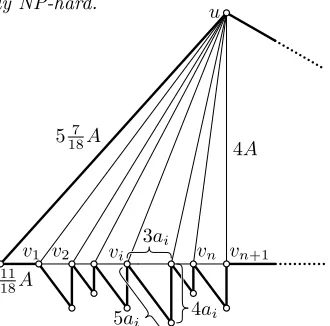
Fig. 4. MinLength instance constructed for instance{a1, a2, . . . , an}of Partition.
Proof. Our proof is by reduction from the weakly NP-complete prob-lemPartition, defined as follows: let
A = {a1, . . . , an} be a set of
posi-tive integers and let A = P ai∈Aai;
is there a set I ⊆ A such that
P
ai∈Iai =A/2? For aPartition
in-stance, we construct a MinLength-Poly instance M with τ = 3 and
the polygonP and triangulationCas shown in Fig. 4, using one last point at distance 7Ato the right of vn+1. We prove that Madmits a solution S of total length at most 3A/2 if and only ifAis a yes-instance of Partition.
LetA={a1, . . . , an} be a yes-instance ofPartitionand let I⊆ Abe such
that P
[image:10.612.314.479.446.609.2]MinLengthinstanceMwith total length at most 3A/2. Every edge{vi, vi+1} ∈
C with i ∈ {1, . . . , n} (i.e., every horizontal edge) is trivially satisfied as P already contains a path of length 3ai. The vertical edge {u, vn+1} is exactly satisfied: walking in counter-clockwise direction alongP yields au-vn+1path of length 15A and every horizontal edge{vi, vi+1} ∈S reduces the length of this path by 5ai+4ai−3ai= 6ai; therefore, the shortestu-vn+1path has total length 15A−6A/2 = 12A = τ4A = τk{u, vn+1}k. Every other edge {u, vi} incident
touis satisfied, because it is longer than{u, vn+1}, while at the same time the shortestu-vipath is shorter than the shortestu-vn+1path. By construction, the selected edges have total length 3A/2.
Now, let S ⊆C be a solution toM of total length at most 3A/2. Because every non-horizontal edge has a length of at least 4A,S contains only horizontal edges. The edge {u, vn+1} can be satisfied only if the total length of horizontal edges inSis at least 3A/2: hence, the total length ofSis exactly 3A/2. Therefore, the numbers inAcorresponding to the edges inS sum up toA/2.
The coordinates of the vertices of the input polygon are rationals—or integer if we scale by a factor of 18—and polynomial in the sumAofA. Therefore, the reduction can be computed in pseudopolynomial time.
Theorem 3. MinWeightPolyis weakly NP-hard.
Proof. We use the same reduction as in the proof of Theorem 2, except that we define the weights as a part of theMinWeightPolyinstance: we set the weight
of each horizontal edge to its length and of each other edge to 4A. All weights are polynomial inA. With this the argument works as before. ut
Since MinLengthPoly and MinWeightPoly are weakly NP-hard, the
more general problemsMinLengthandMinWeightare weakly NP-hard too.
Furthermore, the polygon that we constructed for our reduction admits only one triangulation. Therefore, the problems do not become easier, if we restrict the triangulation implied byC, e.g. to a constrained Delaunay triangulation [6].
Exact solution of MinWeightPoly.The algorithm forMinSizePolycan be
adapted to solve MinWeightPoly, assuming integer weights. Letw:C →N denote the weight function. In the unweighted case, Lemma 2 implies thatleaf
or root assignments with size over |αselfe | −1 are never needed. Its weighted
variant states that, for an edge e, leaf or root assignments with size over
W(αself
e )−w(e) are never needed, whereW(·) denotes the sum of weights over
all edges with aselfassignment. Thus, for each diagonaleandi∈ {1, . . . , w(e)},
we compute aleafassignment with total weight exactlyw(αselfe )−iand
mini-mal front-length. Analogously, we compute up tow(e)rootassignments, with
maximal front-allowance. A straightforward implementation for computing the partial solutions for an edge from its children’s solutions thus takes O(w(e)2) time. Therefore, this algorithm takes O(P
e∈P∪Cw(e)2) ⊆ O(wmax ·wsum) ⊆
O(nw2
max) time, wherewmax= maxe∈Cw(e) andwsum=Pe∈Cw(e).
Letλdenote a small constant and assume 1 +λ≤mine∈Ckek. We define two
weight functions:w(e) = 2λ·round(kek/(2λ)) andw0(e) =round(kek/(2λ)). We
run the weighted algorithm using w0 as its integer weight function. However,w
and w0 are identical up to scaling and thus produce the same optimal results.
The rounding inwimplieskek−λ < w(e)≤ kek+λandw(e)>1 by assumption. LetS denote the result of the algorithm; it has weight w(S) = P
e∈Sw(e)
and lengthl(S) =P
e∈Skek. We find thatw(S)> l(S)−λ|S|> l(S)−λw(S),
implying l(S) < (1 + λ)w(S). Let S∗ denote an optimal solution to
Min-LengthPoly; we find w(S∗) ≤ l(S∗) +λ|S∗| ≤ l(S∗) +λw(S∗) and thus
l(S∗) ≥ (1−λ)w(S∗). The approximation ratio obtained by our algorithm is
l(S)/l(S∗)<(1 +λ)w(S)/((1−λ)w(S∗)). SinceS is optimal in terms of weight,
this simplifies to (1 +λ)/(1−λ).
The running time of this approach is O(nW02) where W0 = max
e∈Cw0(e).
Asw0(e)≤ kek/(2λ) +1
2, we find that this isO(nL2/λ2) whereL= maxe∈Ckek. We thus get a (pseudo)PTAS to approximateMinLengthPoly, that computes
a (1 +ε)-approximation inO(nL2(2+ε ε )
2) =O(nL2/ε2) time.
5
Use Cases
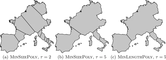
Two vertices lying on opposite sides of a narrow part of a polygon typically have a very large dilation: a connection across the strait of Gibraltar, for example, is much shorter than a path along the coast, all around the Mediterranean Sea. Hence, our dilation-based method may find natural subregions of a polygon. This general hope is confirmed by the results that we obtained with implementations of our algorithms; see Fig. 5. Here we apply our method to two specific problems: computing distorted maps (Section 5.1) and aggregating areas (Section 5.2).
5.1 Computing distorted maps
Several methods exist to distort a map, for example, to resolve spatial conflicts or to emphasize certain information. Such methods often rely on constraints that
[image:12.612.135.476.509.632.2](a)MinSizePoly,τ= 2 (b)MinSizePoly,τ= 5 (c)MinLengthPoly,τ= 5
are defined based on a geometric graph representing the map [10,11]. An edge in this graph may represent a line segment of a map object, but usually additional edges are needed to model the constraints for the output map. We consider our graph augmentation method as a useful tool for finding such relevant edges.
The method of Harrie and Sarjakoski [10] for the resolution of conflicts relies on a constrained Delaunay triangulation of the map objects. A constraint for the length of a triangle edge e = {u, v} is introduced if e is shorter than a thresholdεand the map does not contain au-v path of less than a numberkof line segments. Similarly, our method selects edges of a triangulation based on a geometric distance and a graph-theoretical distance between two vertices of the map. However, while the method of Harrie and Sarjakoski measures the graph-theoretical distance in the input map, our method considers the graph-graph-theoretical distance after augmenting the map with the selected edges. We consider our approach promising as it avoids redundant constraints.
The method of Haunert and Sering [11] enlarges a user-selected focus region in a map while minimizing the distortion, which is measured at the edges of a graph representing the map objects, for example, a network of roads or country borders. Additional edges are necessary if the relative position should be main-tained for some pairs of vertices: e.g., vertices on opposite sides of a strait. To make a good selection of edges, Van Dijk et al. [18] have developed a greedy heuristic that iteratively augments the map with an edge of maximal dilation (among all edges of a constrained Delaunay triangulation) while the dilation of the graph exceeds a certain threshold. In contrast, our linear-time algorithm for polygons makes an optimal selection of multiple edges.
Fig. 6 shows results that we obtained with the method of Haunert and Ser-ing [11] when enlargSer-ing Wales in a polygon representSer-ing Great Britain. For the result in Fig. 6(middle), only distortions of the edges of that polygon were taken into account, which almost caused a collision of England’s east and west coast. A better result is obtained with the additional edges (see Fig. 6(right)): east-west relations are preserved more accurately, yielding a more “solid” deformation.
5.2 Area aggregation
Information on land cover is often given as a planar subdivision that consists of regions of different classes (urban, rural, forest, etc.). To generalize such data, one often aggregates the areas into larger regions such that many-to-one relationships arise. Usually, every output area must have at least a certain minimal size. Subject to this requirement, Haunert and Wolff [12] suggested minimizing a cost function that combines two objectives: the overall weighted class change should be small and the resulting areas should be geometrically compact. They showed that the problem is NP-hard and developed an exact method based on integer linear programming and a heuristic method based on simulated annealing.
Fig. 6.(left) A polygon representing Great Britain with the edges of aMinSizePoly
solution withτ = 2. Variable-scale maps computed (middle) without and (right) with consideration of the selected diagonals. The method of Haunert and Sering [11] was used with a scale factor of 2 for Wales; the results were scaled to the same height.
0 200 m Drestedt
(a) original landscape model (b) result of partitioning polygons in (a)
a
b c
(c) result of aggregating polygons in (a)
a
b c
(d) result of aggregating polygons in (b)
[image:14.612.133.482.352.604.2]requirement for the scale 1:250 000. Observe that several settlement areas (red) are lost. To obtain a better solution, we apply our algorithm for MinSizePoly
with τ = 4 and use its result (Fig. 7(b)) as input for the aggregation method. The solution that we obtain (Fig. 7(d)) is clearly better with respect to the total class change: the relatively large settlement labeled with a is retained. Moreover, more compact shapes have been produced, for example, by filling small concavities in the polygons; see the labelsbandc. Based on the objective function defined by Haunert and Wolff we can quantify this improvement: for a sample of n1 = 325 polygons from ATKIS DLM 50 the aggregation method yielded a solution of 7.1% less total cost when using the polygon partitioning algorithm, which resulted inn2 = 881 polygons. The cost for class change was reduced by 3.2% and the cost for non-compactness by 12.2%. The higher quality comes at the cost of an increased number of input polygons for the aggregation method. Hence, fast heuristics for aggregation are needed and it is reasonable to minimize the number of output polygons when using our polygon partitioning method. In our experiments, we ran simulated annealing with the same very large number (8 810 000 = n2·104) of iterations to produce near-optimal solutions; this took slightly more than half an hour on a desktop PC.
6
Conclusion
We studied the algorithmic problem of augmenting a simple polygon P of n edges by adding edges from an internal triangulation to bound its dilation. We described an optimal linear-time algorithm to minimize the number of edges added. Moreover, we gave anO(nlogd) algorithm for dealing with any crossing-free set C of candidates (d is the maximal number of neighbors of a region induced byP andC) and a heuristic for polygons with holes. Furthermore, we proved that the weighted case and the length-weighted case are weakly NP-hard. We gave anO(nw2
max) algorithm for the former problem (wmax is the maximal weight of an edge) and a (1 +ε)-approximation algorithm for the latter.
We evaluated the benefits of using augmentation in two use cases: distorting maps and area aggregation. When distorting a map to enlarge a focus region, the augmentation leads to a better preserved shape throughout the map. When aggregating areas, it yields 3.2% less class change and 12.2% better compactness.
Future work.Our results leave several interesting open algorithmic problems. E.g., can we construct an algorithm that can deal with a candidate setC that contains intersecting edges, but the solution must be planar? However, this may imply that no solution exists. What if we allow not only internal diagonals of a polygon, but any edge that does not cross the polygon boundary?
We plan to run extensive experiments to further explore graph augmentation for our use cases, to provide guidelines for parameter and weight selection and model the trade-offs between computation time and quality more explicitly.
References
1. B. Aronov, K. Buchin, M. Buchin, B. Jansen, T. de Jong, M. van Kreveld, M. L¨offler, J. Luo, R. I. Silveira, and B. Speckmann. Connect the dot: computing feed-links for network extension. J. Spatial Inf. Sci., 3:3–31, 2011.
2. B. Aronov, M. de Berg, O. Cheong, J. Gudmundsson, H. Haverkort, M. Smid, and A. Vigneron. Sparse geometric graphs with small dilation. Comp. Geom., 40:207–219, 2008.
3. P. Bose and J. Keil. On the stretch factor of the constrained Delaunay triangula-tion. InProc. 3rd Int. S. Vor. Diag. in Sci. & Eng., pages 25–31, 2006.
4. P. Bose and M. Smid. On plane geometric spanners: a survey and open problems.
Comp. Geom., 47(7):818–830, 2013.
5. B. Chazelle and D. Dobkin. Decomposing a polygon into its convex parts. InProc. 11th S. Theory of Comp., pages 38–48, 1979.
6. L. P. Chew. Constrained Delaunay triangulations. Algorithmica, 4(1–4):97–108, 1989.
7. M. Farshi, P. Giannopoulos, and J. Gudmundsson. Improving the stretch factor of a geometric network by edge augmentation.SIAM J. Comp., 38(1):226–240, 2008. 8. H. Y. F. Feng and T. Pavlidis. Decomposition of polygons into simpler compo-nents: Feature generation for syntactic pattern recognition.IEEE Trans. Comput., 24(6):636–650, 1975.
9. P. Giannopoulos, R. Klein, C. Knauer, M. Kutz, and D. Marx. Computing geomet-ric minimum-dilation graphs is NP-hard.Int. J. Comp. Geom. & Appl., 20(2):147– 173, 2010.
10. L. Harrie and T. Sarjakoski. Simultaneous graphic generalization of vector data sets. GeoInformatica, 6(3):233–261, 2002.
11. J.-H. Haunert and L. Sering. Drawing road networks with focus regions. IEEE Trans. Vis. & Comp. Graph., 17(12):2555–2562, 2011.
12. J.-H. Haunert and A. Wolff. Area aggregation in map generalisation by mixed-integer programming. Int. J. Geogr. Inf. Sci., 24(12):1871–1897, 2010.
13. J. M. Keil and J. Snoeyink. On the time bound for convex decomposition of simple polygons. Int. J. Comp. Geom. & Appl., 12(3):181–192, 2002.
14. R. Klein, C. Levcopoulos, and A. Lingas. A PTAS for minimum vertex dilation triangulation of a simple polygon with a constant number of sources of dilation.
Comp. Geom., 34:28–34, 2006.
15. J.-M. Lien and N. M. Amato. Approximate convex decomposition of polygons.
Comp. Geom. Theory & Appl., 35(1):100–123, aug 2006.
16. A. Lingas. The power of non-rectilinear holes. In Proc. 9th Colloquium on Au-tomata, Languages and Programming, pages 369–383, 1982.
17. K. Siddiqi and B. B. Kimia. Parts of visual form: Computational aspects. IEEE Trans. Pattern Anal. Mach. Intell., 17(3):239–251, 1995.
18. T. C. van Dijk, A. van Goethem, J.-H. Haunert, W. Meulemans, and B. Speck-mann. Accentuating focus maps via partial schematization. InProc. 21st ACM SIGSPATIAL Int. C. Advances Geogr. Inf. Syst., pages 418–421, 2013.
19. A. Voisard, M. O. Scholl, and P. Rigaux. Spatial Databases: With Application to GIS. Morgan Kaufmann, 2002.