Three-dimensional numerical simulation of Marangoni instabilities in non-cylindrical liquid bridges in microgravity

AUTHOR’S POST PRINT (Romeo Colour: Green)

Int. J. of Heat and Mass Transfer (ISSN: 0017-9310), 44 (10): 1983-2003 (2001). DOI: 10.1016/S0017-9310(00)00243-X

Publisher version available at

http://www.sciencedirect.com/science/article/pii/S001793100000243X

Three-dimensional numerical simulation of Marangoni instabilities

in non-cylindrical liquid bridges in microgravity

M.Lappa

*

, R. Savino, R. Monti

Università degli Studi di Napoli "Federico II"

Dipartimento di Scienza e Ingegneria dello Spazio "Luigi G. Napolitano" P.le V.Tecchio 80, 80125 Napoli (Italy)

*_{current e-mail address: [email protected]}

Abstract

1. Introduction

The float zone method is an important technique to produce high quality crystal material. By the containerless method, crystals can be grown with less contamination, more homogeneity and higher purity. In these tecniques the melt is positioned and solidified without physically contacting the container's wall in order to minimize container-induced contamination and heterogeneous nucleation.

In the float zone crystal growth, a melt zone is produced by heating a short length of feed rod by a heat source such as a ring heater. The rod is slowly moved through the hot zone, and the crystal is obtained by resolidification of the melt as it is moved away from the melt zone. If the melt/crystal interface remains flat during the resolidification, often uniform and high quality single crystals can be produced.

The float-zone technique under microgravity seems to be a promising crystal growth method to solve several problems. Buoyancy driven convection which is the most important cause of micro-inhomogeneities (striations) is in fact absent under microgravity conditions. Furthermore, because of the limitations set by hydrostatic pressure on earth, crystals with a larger diameter can be grown by this technique only under zero g conditions.

The availability of extended periods of microgravity in Earth-orbiting laboratory as the Spacelab and the Space Station has made interesting experiments and manufacturing processing possible, which hardly could be performed on Earth under normal gravity conditions.

However, even in the absence of gravity the presence of free-melt-gas interface at different temperatures induces thermocapillary convection, the so-called Marangoni convection.

The appearance of instabilities of Marangoni flow in these configurations may lead to the appearance of undesirable imperfections (e.g. dopant inhomogeneities) in the final crystals; consequently non-isothermal liquid bridges have received much attention during the past years. The development of supercomputers and efficient numerical methods led the investigators to study the problem through direct numerical solution of the non linear and time-dependent Navier Stokes equations.

Rybicki and Florian [1] considered the steady axisymmetric thermocapillary convection in cylindrical liquid bridges. They analyzed numerically the effects of the bridge aspect ratio showing that a decrease in the aspect ratio (short bridges) leads to the emergence of several layers of vortices, with the strenght of each layer decreasing approximately exponentially with the distance from the surface.

Rupp et al. [2] were the first to develop a 3D numerical code able to simulate the transition of Marangoni flow in cylindrical half zone configurations. They studied the behaviour of the instability for several low Prandtl liquids and for a fixed aspect ratio, and found that for liquid metals the first bifurcation is stationary (i.e. the supercritical three-dimensional state is steady) and that the regime becomes oscillatory only when the Marangoni number is further increased (second oscillatory bifurcation). These results pointed out that the behaviour of the Marangoni flow instability for low Prandtl liquids is different compared to the high Prandtl cases.

Levenstan and Amberg [3] analyzed, for a fixed small Prandtl number (Pr=0.01) and for a fixed aspect ratio, the nature (i.e. the physical explanation) of the first steady and of the second oscillatory bifurcation of the Marangoni flow. More recently Lappa and Savino [4] studied the azimuthal structure of the flow pattern that is established after the steady bifurcation for Pr=0.04 and for two different values of the geometrical aspect ratio (A=L/D). They showed that there is a strong relation between the value of A and the critical azimuthal wave number (m) of the instability.

Kuhlmann [5], Kuhlmann and Rath [6], Wanschura et al. [7] investigated the linear stability of steady axisymmetric thermocapillary flow in cylindrical liquid bridges. Their results predicted the critical Marangoni numbers and the form of the most typical disturbances, characterized by the appropriate value of the critical wave number, in the neighbourhood of the neutral stability point (i.e., close to the onset). Comparison of the theoretical results with the numerical available data have confirmed some features of the observed instabilities, e.g., for low Prandtl numbers the instability breaks the spatial axisymmetry (but the flow regime is still steady) prior to the onset of time dependent flow field, whereas for high Prandtl numbers the instability is oscillatory (Hopf bifurcation).

All the available three-dimensional numerical results have been obtained for cylindrical liquid bridges.

It is expected that both the aspect ratio (A) and the shape factor S=V/Vo, where V is the liquid volume and Vo is the volume of the cylindrical liquid bridge (Vo=LR2_{, where R is the radius of}

the supporting disks and L is the length of the liquid bridge), should influence the Marangoni instability occurrence.

Chen and Hu [10] used the linear stability analysis to study the influence of the liquid bridge volume on the instability of Marangoni flow for high Prandtl number liquids.

This overview of the literature on the subject shows that there is still a lack of three-dimensional numerical results about the behaviour of Marangoni flow in non cylindrical liquid bridges. In particular, it is unknown how the stability limits depend upon S1 for low Prandtl liquids.

In the present paper the influence of the shape factor of the liquid bridge on the critical parameters (critical Marangoni number and critical azimuthal wave number) for semiconductor melts under zero-g conditions is studied through direct numerical solution of the three-dimensional, non linear and time-dependent Navier-Stokes equations.

2. Physical and mathematical model

2.1 Basic assumptions

The geometry of the problem is shown in Fig. 1. An axisymmetric liquid bridge of length L and diameter D is held between two coaxial disks at different temperatures. The upper disk in Fig.1 is kept at the temperature TH higher than the temperature TC of the lower cold disk. The imposed temperature difference is denoted by T ( TH TC  T . The overbar denotes dimensional quantities. The liquid is assumed homogeneous and Newtonian, with constant density and constant coefficients; viscous dissipation is negligible. The liquid filling the bridge is bounded by an axisymmetric liquid-gas interface with a surface tension  exhibiting a linear decreasing dependence on the temperature:



 



o





T

(

T T



o

)



(1)

where o _{is the surface tension for T}  T0 and T  d/dT > 0.

The interface is assumed to be nondeformable and axisymmetric around the z-axis; its radial coordinate is a function of the z variable (r g z( )).

At zero g, the hydrostatic shape of this surface can be obtained from the Gauss-Laplace equation, relating the local curvature of the surface to the pressure jump along the liquid-gas interface:

   

 

 



2 1

1 1

R R

whre R₁ and R₂ are the principal radii of curvature at each point of the surface.

Equation (2) may be reformulated in dimensionless form in the cylindrical co-ordinates by substituting the analytical expression of the principal radii of curvature in axi-symmetric geometry in terms of the surface equation g(z) (g g L / , r r L/ , z z L/ ):

1

1 2 1 2 3 2

g g

g g

L p _k ( ' )

'' ( ' ) /

      (3a)

where the left hand side represents the non-dimensional pressure jump with respect to the capillary pressure /L. Equation (3a) can be written as :

gg''_kg(_1g' )2 3 2/ _{ }(₁ g' )2 1 2/ _0

_(3b)

Each value of the parameter k  L p/ corresponds to a shape and to a fixed volume of the liquid bridge. The value of k has been assigned in equation (3b) (to obtain the desired shape for each case considered) and the equation has been integrated by a shooting method with the conditions that the liquid is attached to the solid supports:

g(0) = g(1) = R/L (4a b)

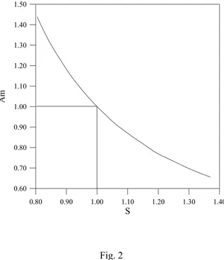
Further to the non-dimensional liquid bridge volume (or shape factor S=V/Vo) and to the geometrical aspect ratio (A=L/D), other geometrical parameters are introduced: Dm minimum or maximum diameter of the liquid bridge , and the non-dimensional parameter Am=L/Dm , ratio of the length of the bridge to the minimum or maximum diameter (this parameter is not independent of A and S as shown in Fig.2 for A=1).

2.2 Nondimensional field equations and boundary conditions

The flow is governed by the continuity, Navier-Stokes and energy equations, that in non-dimensional conservative form read :

 V 0 (5a)

 

V

t    p VV Pr 2 V (5b)

 

T

t   VT   T

where V, p and T are the non-dimensional velocity, pressure and temperature, Pr is the Prandtl number. The non-dimensional form results from scaling the cylindrical co-ordinates (r z, ) by the axial distance between the circular disks (L) and the velocity components (u v V, , ) by the energy

diffusion velocity V = /L; the scales for time and pressure are, respectively, L/ and /L( being the thermal diffusivity). The temperature, measured with respect the initial temperature T0 , is scaled by (T):

T= (T T 0) / (T) (6)

In cylindrical co-ordinates the momentum equations read:

                    

 uV

r r uv r uv z u z p t

u 2 1

        

Pr 2₂ 2₂ 1 1₂ 2₂

        u r r u r r u z u (7a)                r V vV r r v r v z uv r p t

v 2 2 2

1  

                              

 V

r v r r v r r v r v z v 2 2 2 2 2 2 2 2

2 _{1 1 2}

Pr (7b)                     

  1   2  1 V2

r r vV r vV z uV p r t V                       

 _{     v}

r V r r V r V r r V z V 2 2 2 2 2 2 2 2 2 2 1 1 Pr (7c)

At the initial time the liquid filling the bridge is supposed to be quiescent and at uniform temperature:

t=0: V(z, r, ) = 0 , T (z, r, )= 0 (8)

For t > 0, the boundary conditions on the rigid disks are the no-slip condition and the temperature conditions:

on the cold disk

V (z=0, r,  _{, t) = 0;} (z=0, r,  , t) = 0 0 r 1 2/ A ; 0  2 (9)

on the hot disk

The boundary conditions on the free surface (r=g(z)) are the kinematic conditions of a stream surface (zero normal velocity), the Marangoni conditions (shear stress balance) and the adiabatic condition.

Hereafter V_s and V_n denote the velocity components in the plane (r-z) parallel and orthogonal to the free surface respectively:

VS u z r( , g z( ), , ) t v z r( , g z( ), , ) t (11a) Vn u z r( , g z( ), , ) t v z r( , g z( ), , ) t (11b)

where  and  are the components of the unit vector orthogonal to the free surface along z and r respectively.

The condition of zero normal velocity and the Marangoni conditions read: Vn  0 v z r( , g z( ), , ) t   u z r( , g z( ), , )t



 

(12a)



Vn Ma 

T

s z r g z t

s _{  ( ,  ( ), , ) (12b)}

r V

r z r g z t V z r g z t Ma T

z r g z t  

  



 



( ,  ( ), , ) ( ,  ( ), , )   ( ,  ( ), , ) (12c)

where the reference Marangoni number Ma is defined as Ma=_T(T)L/. The adiabatic condition is written as:



 



 

  T

n

T z

T r

  0 (12d)

To solve the problem, the body-fitted curvilinear coordinates are adopted. The non cylindrical original physical domain in the (r,z,) space is transformed into a cylindrical computational domain in the (,,) space by

z

r g

 



 ( )





 

 

z

r g/ ( )

(13)

thus the radial coordinate r ranges from =0 (at the symmetry axis) up to =1 at the free surface; the axial coordinate varies from =0 at the cold up to =1 at the hot disk.

The first order spatial derivatives read 

  

 

 

  f

z f

z f

z

 





 

 

  f

z

f g g

f

  '

(14a)



fr     f

r f

r

 







  f

y g f

The second order spatial derivatives read              f g g f g g f g g f z

f ' 2 ' 2 ''

2 2 2 2 2 2 2 2           (15a)    2 2 2 2 2 1 f r g f



(15b)

Thus the field equations read:             u g g u g v v g g V

 ' 1   1 0 (16a)

                                      

 uV

g g uv uv g u g g u P g g P t

u ' 2 ' 2 1 1

                                   2 2 2 2 1 '' 1 2 ' 2 2 2 1 ' 2 2

Pr _{2 2}

2                u g u g g g u g g u g g g u

(16b)                                     

  vV

g g V g v v g uv g g uv P g t

v 1 ' 1 2 2 2 1

                                                      

 V

g v g g v v g g g v g g v g g g v 2 2 2 2 2 2 2 1 2 2 '' 1 2 ' 2 2 2 1 ' 2 2

Pr _{2 2}

2 (16c)                                    

 _{     }2

1 2 1 ' 1 V g g vV vV g uV g g uV P g t V                                                       

 _{     } v

g V g g V V g g g V g g V g s g V 2 2 2 2 2 2 2 1 2 2 '' 1 2 ' 2 2 2 1 ' 2 2

Pr _{2 2}

2 (16d)                        

 VT

g g vT vT g uT g g uT t

T ' 1 1

The derivatives in the boundary condition (12b) can be expressed as         T s T z T r

  0 

                   T g g g T T g T g g T s T                 

 ' 1 1 ' (17a)





n u v u n n V_S                    

 2  

     _         r u z u n V_S            2                                 u g u g g u n

V_S 2 ' 1

(17b)

and substituting the (17a) and (17b) into the (12b):

             u g g g ' 1                                    

 1 ' T / 2

g g g T Ma u (18)

The adiabatic condition on the free surface (12d) in the (,) plane reads:         g g g T

T

/

_ '_{ } 1

     (19)

3. Numerical solution

3.1 The numerical method

Equations (16a-e) subjected to the initial and boundary conditions were solved numerically in the transformed space (,,) in primitive variables by a finite-difference method. The transformed domain was discretized with a uniform cylindrical mesh and the flow field variables defined over a staggered grid. Forward differences in time and central-differencing schemes in space (second order accurate) were used to discretize the partial differential equations, obtaining:

 

_{VV V t p}n

t V V

n n

n _{ }

                 2 Pr 1 (20)

 

n

n

n _{T t VT T}

T                

1 2 ₍₂₁₎

In the first, an approximate velocity field V* corresponding to the correct vorticity of the field, but with  V*_{0, is computed at time (n+1) neglecting the pressure gradient in the momentum} equation, i.e.,

 

n

n

V V

V t

V V

    

  

  

   

 Pr 2

* (22)

In the second substep, the pressure field is computed by solving a Poisson equation resulting from the divergence of the momentum equation with the help of the continuity equation:

2_pn  1 t V

*

(23)

Finally, the velocity field is updated using the computed pressure field to account for continuity:

Vn1 _V*_{ }t pn ₍₂₄₎

The Poisson equation is solved with a SOR (Successive Over Relaxation) iterative method. The temperature field at time (n+1) is obtained from eq. (21) after the calculation of the velocity. For more details on the numerical method see e.g. Lappa and Savino [4] and Fletcher [11].

The critical Marangoni numbers for the first steady and for the second oscillatory (Hopf) bifurcation are denoted respectively with Ma_c1 and Ma_c2.

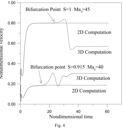
The first critical Marangoni number (Ma_c1) has been determined for each study-case considered in the computations by monitoring the time temperature and velocity profiles in a specially defined grid point near the surface of the liquid bridge (=0.75, =0.9, =). Before the transition point the temperature profiles obtained with 2D and 3D numerical computations are coincident. After the onset of instability the results of the 3D code depart from 2D computations, due to the symmetry breaking and to the three-dimensional flow field organization.

A similar procedure can be used to obtain the value of the second critical Marangoni number (Ma_c2), the criterion being based in this case on the onset of time oscillations in the profiles of temperature and velocity rather than on the onset of three-dimensional flow.

3.2 Validation of the numerical procedure

The numerical prediction of convective instabilities requires a very careful investigation (see e.g. Ref. [12]). For this reason the numerical model has been validated by quantitative comparisons with 2D and 3D numerical results (S=1) for Prandtl numbers as close to the one used in the present work as possible.

For two-dimensional computations, the stream function minimum of the axisymmetric flow in the case A=0.5, Pr=0.1 and Ma=10 is compared with the results reported by Wanschura et al. [7]. Table Ia shows that values obtained with the present code compose very well with those by Wanschura et al. [7].

To check that the code is able to "capture" the physical instabilities of Marangoni flow, the critical Marangoni number in the case A=0.5 and Pr=0.01 has been computed and compared with the results of Levenstam and Amberg [3]. For this case they predict Mac120 (using as reference length the length L of the bridge, according to the present non-dimensionalization). The critical Marangoni number determined by the present numerical computations is Mac121 (6% greater than their value) with m=2. These comparisons provides a sufficient validation of the present numerical code.

3.3 Grid refinement study

In this sub-section in order to show the numerical convergence of the present algorithm a grid refinement study is presented .

of collocation points in the axial direction, and the second define the grid size in the radial direction).

Wanschura et al. [7] found grid convergence for a resolution of 25 x 14 points. In the present paper

grid convergence has been obtained for a resolution of 22 x 22 points (the value obtained for 32 x

32 is 0.5% larger than the value obtained for 22 x 22).

The grid refinement study has been conducted also on the influence of the number of points used in azimuthal direction. Table Ib shows that for the case Pr=0.01 and A=0.5 grid convergence can be obtained using 20 points in azimuthal direction (the computed Mac1 does not change increasing the grid resolution).

4. Results and discussion

Because of the considerable computation time involved (for a stable supercritical flow solution after the bifurcation point about 50 cpu hours on a Silicon Graphics Power Challenge super computer were needed for each case considered) the investigation has been restricted to only one value of the Prandtl number (Pr=0.01) but different aspect ratios have been investigated for several values of the shape parameter S under zero-g conditions.

All the results have been obtained using 22 x 22 points in the r,z plane and 30 points in the azimuthal direction, whatever is the aspect ratio or the shape factor. Figs.3 show some computational grids used in this work.

4.1 The steady bifurcation

The transition process for all the cases investigated seems to substantiate typical features of the theory of steady bifurcations.

In the axisymmetric state (prior to the transition) the fluid-dynamic field corresponds to an axisymmetric toroidal vortex. The supercritical state can be interpreted as the superposition of a steady sinusoidal azimuthal disturbance to the axisymmetric field, i.e., the generic flow field variable F(r, z, ) can be expressed as:

F(r, z,  _{) = Fo(r, z) +} F~(r, z) sin (m + G) (25)

where the subscript (o) refers to the axisymmetric field, m is the azimuthal wave number (from a physical point of view m represents the number of sinusoidal distortions in azimuthal direction), F  is the perturbation amplitude and G is a constant phase shift due to the fact that the azimuthal position of the disturbances is random.

The solution shows that the position of the vortex core after the bifurcation is displaced sinusoidally along the azimuthal perimeter of the liquid zone and the temperature field is characterized by sinusoidal distortions in azimuthal direction.

This result was confirmed in this paper by subtracting the azimuthally averaged flow field from the total flow field obtained numerically. Hereafter, the temperature fields obtained as differences between the numerical three-dimensional solutions and the corresponding averaged fields will be referred to as temperature disturbances (see for instance Figs.8 and 14).

4.2 Influence of the aspect ratio

For cylindrical liquid bridges the numerical computations have shown that the flow structure of the supercritical state depends on the value of the aspect ratio. The lower the aspect ratio, the higher the critical azimuthal wave number m resulting in the more complex flow organization.

When m increases multicellular structures are formed. In the generic section orthogonal to the z axis 2m convective cells are present and on the bridge free surface 2m temperature spots (m cold and m hot) appear (Figs. 8a, 14a and 20a).

there are two asymmetrical vortex cells in each meridian plane of the liquid bridge (one of the two vortex cells in the section prevails over the other and is extended along the whole axial plane of the bridge, for instance see Fig.9a and 21a). For even critical wave numbers, the flow field structure is on the whole three-dimensional and depends on the azimuthal co-ordinate, but in each meridian plane the velocity and temperature are symmetric (for instance see Fig.15a).

The present results obtained for S=1 (see Table IIa) suggest an empirical correlation between the geometrical aspect ratio and the critical azimuthal wave number of the instability. For Pr=0.01 and cylindrical liquid bridges this correlation is

mA



1

(26)

These findings are in agreement with previous results as shown in Table IIb where the critical wave numbers for low Prandtl number liquids and different aspect ratios are summarized.

Rupp et al. [2] found m=2 for A=0.6 and for Pr ranging from 0.007 to 0.16, but they did not make a study on the influence of the geometrical aspect ratio (A). Levenstam and Amberg [3] found m=2 for A=0.5 and Pr=0.01. Lappa and Savino [4] found m=1 and m=2 for A=1.0 and A=0.6 respectively (Pr=0.04).

Wanschura et al. [7] gave the dependence of the most "dangerous" azimuthal wavenumber on the aspect ratio for Pr=0.02. They found that as the aspect ratio decreases, modes with higher azimuthal wavenumber m become critical. In their results the most dangerous mode is m=1 for 1.5>A>0.8, m=2 for 0.75>A>0.4, m=3 for 0.35>A>0.28 and m=4 for 0.28>A>0.25 in good agreement with the present results.

4.3 Influence of the shape

The computations performed considering a non cylindrical surface point out that the shape parameter S influences both the critical Marangoni number and the critical azimuthal wave number (see Table III).

and Fig. 6a) and two thermal spots (Fig. 7a). Moreover two thermal spots are present on the liquid bridge surface (Fig. 8a).

When a non-cylindrical shape is considered (S1), the first critical Marangoni number is lower for S>1 (convex bridge) and higher for S<1 (concave bridge). For instance the critical Marangoni number becomes Ma_c1=30 for S=1.22 and Ma_c1=47 for S=0.78 .

For A=1 m = 1 for S=1 (and for S<1); and m=2 for S=1.22 (fat liquid bridge).

In the generic cross-section orthogonal to the liquid bridge axis there are two azimuthal convective cells and two thermal spots on the liquid bridge surface for S=1 but for S=1.22 the convective cells and the temperature spots are four (Figs. 5b, 6b and 7b) and there are four thermal spots on the free surface (two hot and two cold, Fig. 8b). Moreover comparing Fig. 9a and Fig. 9b it is evident how in the first case the flow pattern in the generic meridian plane is asymmetric (due to an odd mode of supercritical convection) whereas in the latter it is symmetric (due to an even mode of supercritical convection).

For A=0.75 and cylindrical shape the critical Marangoni number is Ma_c1=27 and the critical wave number is m=2 (Figs. 11a-14a).

Similarly to the situation analysed for A=1, for A=0.75 the first critical Marangoni number for S=1 exhibits a higher value for S<1 (concave bridge) and lower value for S>1 (convex bridge). The first critical Marangoni number becomes in fact Ma_c1=33 for S=0.83 and Ma_c1=24 for S=1.167. However in this case, in contrast with the result found for A=1, the critical mode number does not change when the volume is increased and is shifted to a lower value (m=1) when the volume of the liquid bridge is reduced (concave liquid bridge S=0.83, Figs. 11b-14b ). Comparing Fig. 15a and Fig. 15b it is evident in fact how in the first case the flow pattern is symmetric whereas in the latter it is asymmetric.

In contrast with the behaviour observed for A=1 and for A=0.75, for A=0.35 the first critical Marangoni number for S=1 exhibits a higher value for S>1 (convex bridge) and a lower value for S<1 (concave bridge). The first critical Marangoni number is 45 for S=1 and becomes Ma_c1=40 for S=0.915 and Ma_c1=50 for S=1.085.

azimuthal convective cells and six temperature spots, and six thermal spots on the liquid bridge surface for S=1 (Figs. 17a, 18a, 19a and 20a) but for S=0.915 the convective cells and the temperature spots are four (Figs. 17b, 18b and 19b) and there are four thermal spots on the free surface (one hot and one cold, Fig. 20b). Moreover comparing Fig. 21a and Fig. 21b it is evident how in the first case the flow pattern is asymmetric (due to a critical wave number m=3) whereas in the latter it is symmetric (due to a critical wave number m=2).

The results discussed above show that the influence of the non-cylindrical shape on the Marangoni instability in low Prandtl number liquids is different compared to the case of high Prandtl number liquids, where the curve of the critical Marangoni number exhibits a maximum, versus the parameter S, depending on the aspect ratio (see e.g. Hu et al. [13] and Chen et al. [10]).

4.4 Discussion

In the previous paragraphs it has been pointed out that the critical azimuthal wave number increases when the geometrical aspect ratio of the bridge is decreased (section 4.2) and that, for a fixed aspect ratio, it can be shifted to higher values by increasing the volume or to lower values by decreasing the volume (section 4.3).

In particular the numerical results predict m=1 for A=1, m=2 for A=0.75, and m=3 for A=0.35 if S=1; moreover m=2 for A=1.0 and S=1.22, m=1 for A=0.75 and S=0.83 and m=2 for A=0.35 and S= 0.915.

All these results can be summarized with a simple formula if the geometrical parameter defined as Am=Dm/L is introduced; in fact: m=1 for A=1 (S=1) and Am=1 (A=0.75, S=0.83), m=2 for A=0.75 (S=1) and Am=0.75 (A=1, S=1.22) and m=2 for A=0.4 (S=1) and Am=0.4 (A=0.35, S=0.915).

Until now all the theoretical-empirical laws introduced to correlate the critical azimuthal wave number to the geometry of the liquid zone have been formulated considering the relation between the mode number and the geometrical aspect ratio of the zone defined as L/D in order to have m as a function of the characteristic lengths of the liquid zone.

is hydrodynamic in nature, since it does not depend on the behaviour of the temperature field (for this instability the temperature field simply acts as a driving force for the velocity field), the selection rule is given simply by the constraint that the azimuthal wavelength must be an aliquot of the toroidal vortex core circumference (as stated by Chun et al. [14]) and by the fact that the convection roll is limited axially by the presence of the sidewalls (as stated by Xu and Davis [15]). According to this theory the critical wave number should be related to the axial length of the zone and to the diameter D_V of the center-line of the convection roll, i.e. it should scale with the parameter A_V=D_V/L.

Preliminary computations concerning the case of axisymmetric Marangoni flow (Ma<Mac1), performed in order to study the effect of the surface shape on the features of the stable Marangoni convection, have shown that for all the cases investigated (0.3<A<1.3, S=1 and S1), the center of the Marangoni toroidal vortex is located at a distance from the symmetry axis ranging between 72% and 79% of the minumum (or maximum) radius of the bridge (0.75) and at a distance from the cold disk of 40-41% (0.4) of the axial length of the bridge (for instance see Figs. 23 and 24). On the basis of these results an average correlation law can be introduced:

D*=D_V/Dm0.75 (27)

where D_V is the diameter of the toroidal convection roll.

The finding that D*does not change for different values of S (including S=1) is very important because it makes possible to explain the results concerning the three-dimensional Marangoni instability in non-cylindrical liquid bridges.

For cylindrical liquid bridges (27) reads:

D*=D_V/D0.75 (28)

and substituting (28) in (26) : mA mL

D m

L D

D D V

V

  1  m L DV

1 33. mAV 1 33. (29) with A L

D

Since (29) is based on the real diameter of the toroidal vortex, on the basis of the discussion reported above, it can be generalized to the case of non-cylindrical liquid bridges so that it is possible to write

m L

D m

L D

D D

V m

m V

1 33.   mAm 1 (30)

obtaining thus a generalized form of the (26).

These findings also shed some light on the behaviour of the first critical Marangoni number. It has been shown that the first critical Marangoni number is increased for concave bridges and decreased for convex bridges when A=1 and A=0.75 and vivecersa it is decreased for concave bridges and increased for convex bridges when A=0.35.

These particular results can be explained considering that the thermo-fluid-dynamic field (in particular the Marangoni toroidal vortex) is characterized, as discussed above, by the parameter Am rather that A=L/D so that if two bridges have the same Am (i.e. a cylindrical bridge has a geometrical aspect ratio equal to the parameter Am of a bridge having deformed surface) their instability will behave in a similar way and the critical Marangoni numbers will be very similar. The critical Marangoni number as a function of the geometrical aspect ratio A is shown in Table IIa in the case of cylindrical surface. The critical Marangoni number is an increasing function of the aspect ratio for A>0.6 and a decreasing function for A<0.6 reaching a minimum for A=0.6.

For A>0.6 and cylindrical surface for a fixed value of A=L/D if Am is decreased (convex bridge) the bridge behaves as a lower aspect ratio liquid zone and consequently its critical Marangoni number is decreased, viceversa if Am is increased (concave bridge) the bridge behaves as a higher aspect ratio liquid zone and consequently its critical Marangoni number is increased. A completely opposite behaviour happens for A<0.6 since in this case the critical Marangoni number is a decreasing function of the aspect ratio.

4.5 Second transition from steady to oscillatory flow: comparison with experimental results

All the results presented above refer to the first transition (from the steady symmetric to the steady asymmetric organization). If the Marangoni number across the bridge is further increased a second transition occurs at Ma_c2 from the steady to unsteady periodic flow field.

Different with the first transition, this second transition can be detected experimentally by monitoring the temperature time history at fixed points in the bridge. Because of experimental difficulties only few data on this second bifurcation are available.

Tao and Ku [16] investigated Marangoni convection in a liquid bridge (half zone) of tin.

They estimated the critical Marangoni number by looking at the onset of oscillations of temperature measured by thermocouples inserted in the liquid; therefore information are available only for the second (oscillatory) bifurcation.

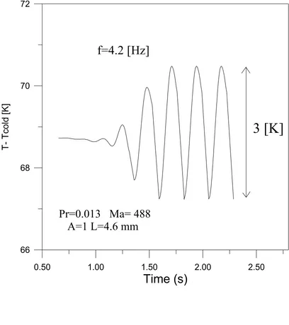
Tin was selected as the material for study in view of its relatively low melting point and well documented physical properties (Pr =0.013). The experiment was conducted in a vacuum chamber in order to prevent oxidation. A liquid bridge of tin was held between two vertical coaxial iron rods 4.5 mm in diameter and 4.6 mm apart (A1). A flow oscillation (with a frequency f=5 [Hz]) was observed (using thermocouples inserted in the liquid) at a temperature difference of 85 [K] (corresponding to a Ma=488). The peak to peak temperature amplitude oscillation was found to be 2.6 [K].

This case has been simulated in the present work for comparison.

For Pr=0.013, A=1, S=1 a first steady bifurcation occurs at Ma_c136 with m=1 and a second Hopf bifurcation at Ma_c275 with m=2.

In addition, it must be pointed out that the procedure employed during the experiments is different from the one used in the present work. Typically the critical Marangoni number is measured by establishing a temperature ramp that increases with time the temperature difference across the bridge. It has been shown in previous papers (Savino and Monti [17]) that unsteady effects, related to the temperature ramp, may postpone the transition point so that the instantaneous Marangoni number, at which temperature oscillations occur, may be larger compared to the one predicted by stability analysis and by numerical simulations that assume an initial steady state.

The numerically computed oscillation frequency and the amplitude of the temperature oscillations obtained for Ma=488 (Fig.25) were found to be f=4.2 [Hz] and 3 [K] respectively (in sufficient agreement with the experimental results obtained in 1-g conditions by Tao and Ku [16] who found a frequency of about 5 [Hz] and a temperature amplitude of about 2.6 [K]).

The spatio-temporal behaviour of the thermofluid-dynamic field was found to be very similar to a "standing wave regime", characterized by the "pulsation" in time of surface temperature spots (hot spots grow during the shrinking of cold spots and viceversa). This behaviour has been observed and explained in many works related to high Prandtl liquids [6, 18-19].

5. Conclusions

A numerical code has been developed which is able to give a direct three-dimensional and time-dependent simulation of Marangoni flow instability in liquid bridges with deformed surface in microgravity conditions.

In this paper the attention has been focused on the case of low Prandtl number liquids, e.g. semiconductor melts, due to their particular relevance in the containerless method of floating zone crystal growth. The numerical results have been analyzed and interpreted in the general context of the bifurcations theory. It has been shown that for semiconductor melts the first bifurcation is characterized by the loss of spatial symmetry rather than by the onset of time-dependence and that, when the basic axisymmetric flow field becomes unstable, after a short transient, a three-dimensional supercritical steady state is reached.

The numerical results have shown that for a fixed aspect ratio the critical azimuthal wave number can be shifted to higher values by increasing S (convex shape) or to lower values by decreasing S (concave shape).

These behaviours have been explained considering the relation between the nature of disturbances and the radial and axial extension of the Marangoni toroidal vortex.

A generalized empirical correlation between the critical azimuthal wave number and the nondimensional geometrical parameter Am has been introduced.

Based on the results of present paper, there are at least two critical geometrical parameters which must be considered when non-cylindrical liquid bridges are investigated in zero-g conditions, that are the geometrical aspect ratio A and the shape factor S.

The second oscillatory (Hopf) bifurcation has been studied for A=1 and S=1 in order to compare the numerical results with experimental ones available in the literature. In particular, the computed frequency and temperature oscillations amplitude are in sufficient agreement with the experimental results obtained by Tao and Ku [16] with a liquid bridge of molten tin in 1-g conditions.

The main features of the three-dimensional flow have been discussed in terms of vector plots, isotherms, and thermal distortions with respect to the basic axisymmetric field. The flow field organization, in the transversal cross-sections, in the axial planes and on the cylindrical free surface have been illustrated, for different critical wave numbers corresponding to different values of the geometrical aspect ratio of the liquid bridge and/or to different shapes of the free surface (convex or concave).

6. Acknowledgments

This work is part of the PhD thesis of M.Lappa.

References

[1] A. Rybicki, J.M. Florian, Thermocapillary effects in liquid bridges. I. Thermocapillary convection, Phys. Fluids, 30, 1956 (1987)

[2] R. Rupp, G. Muller, G. Neumann, Three dimensional time dependent modelling of the Marangoni convection in zone melting configurations for GaAs, Journal of Crystal growth, 97, 34 (1989)

[3] M. Levenstam, G. Amberg, Hydrodynamical instabilities of thermocapillary flow in a half-zone, J. Fluid Mechanics, 297, 357 (1995)

[4] M. Lappa , R. Savino, Parallel solution of three-dimensional Marangoni flow in liquid bridges,

Int. J. Num. Meth. Fluids, 31, 911 (1999)

[5] H.C. Kuhlmann, Some scaling aspects of thermocapillary flows, Microgravity Quarterly, 5, 29 (1995)

[6] H.C. Kuhlmann, H.J. Rath, Hydrodinamic instabilities in cylindrical thermocapillary liquid bridges, J.Fluid Mech., 247, 247 (1993)

[7] M. Wanschura, V. Shevtsova, H.C. Kuhlmann, H.J. Rath, Convective instability mechanism in thermocapillary liquid bridges, Phys. Fluids, 5, 912 (1995)

[8] V. Shevtsova, H.C. Kuhlmann, H.J. Rath, Thermocapillary convection in liquid bridges with a deformed surface, 46th Congress of the International Astronautical Federation, Oslo, Norway, October 2-6 1995

[9] V. Shevtsova, J.C. Legros, Influence of the free surface shape on stability of liquid bridges, Joint Xth European and VIth Russian Symposium on Physical Sciences in Microgravity, St. Petersburg, Russia, 15-21 June 1997

[10] Q.S. Chen, W. R. Hu, Influence of liquid bridge volume on instability of floating half zone convection, Int. J. Heat Mass Transfer, 41, (6-7), 825 (1998)

[12] B. Roux (editor), Numerical simulation of oscillatory convection in low-Pr fluids, A GAMM Workshop, Notes on Numerical Fluid Mechanics, Vieweg (1990)

[13] W.R. Hu, Z.M. Tang, J.Z. Shu, R. Zhou, Influence of liquid bridge volume on the critical Marangoni number in thermocapillary convection of half floating zone, Microgravity Quarterly5, 67 (1995)

[14] C.H. Chun, W. West, Experiments on the transition from the steady to the oscillatory Marangoni convection of a floating zone under reduced gravity effect, Acta Astronautica, 6, 1073 (1979)

[15] J.J. Xu, S.H. Davis, Convective thermocapillary instabilities in liquid bridges, Phys. Fluids, 27, 1102 (1984)

[16] Y. Tao, S. Kou, Thermocapillary convection in a low Pr material under simulated reduced gravity conditions, Third Microgravity Fluid Physics Conference (1996), NASA cp 3338, 301 [17] R. Monti , R. Savino, Effect of unsteady thermal boundary conditions on Marangoni flow in liquid bridges, Microgravity Quarterly, 4, 163 (1994).

[18] S. Frank , D. Schwabe, Temporal and spatial elements of thermocapillary convection in floating zones, Experiments in Fluids, 23, 234 (1998).

Grid size

Minimum stream function

Wanschura et al.[7] 25

x

14

-0.107

Wanschura et al.[7] 50

x

25

-0.107

Present results 22

x

22

-0.1055

Present results 32

x

32

-0.10570

Present results 42

x

42

-0.10578

Present results 52

x

52

-0.10580

Table Ia

Minimum stream function of the axisymmetric flow as a function of mesh spacing

(Pr=0.1, Ma=10)

Grid size

Ma

_c1

m

22

x

22

x

20

21.5

2

22

x

22

x

30

21.3

2

22

x

22

x

40

21.2

2

Table Ib

3D grid refinement study for A=0.5, Pr=0.01

0.0 0.1 0.2 0.3 0.4 0.5 0.6 0.7 0.8 0.9 1.0 1.1 1.2 1.3 1.4 1.5

Table IIb

A Ma

_c1

m

0.2

50

4

0.25 47 3

0.35 45 3

0.4 35 2

0.6 25 2

0.75

27

2

0.8 30 2

0.85 32 2

0.9 33 1

1

35

1

1.25 45 1

Table IIa

Ma

_c1

and m versus the geometrical aspect ratio (S=1)

A=L/D Am S Ma

_c1

m

1.0 1.5 0.78 47 1

1.0 1.0 1.0 35 1

1.0 0.75 1.22 30 2

0.75 1.0 0.83 33 1

0.75 0.75 1.0 27 2

0.75 0.60 1.17 24 2

0.35 0.4 0.915 40 2

0.35 0.35 1.0 45 3

0.35 0.31 1.085 50 3

Table III

Nomenclature

A

aspect ratio, L/D

Am L/Dm Av L/Dv

D

diameter of the supporting disks

Dm

minimum (maximum) diameter of the liquid bridge

Dv

diameter of the toroidal convection roll

g

dimensionless radial coordinate of the free surface

L

height of the liquid bridge

m

azimuthal wave number

Ma

Marangoni

number

Ma_c1

critical Marangoni number for the first (steady) bifurcation

Ma_c2

critical Marangoni number for the second (Hopf) bifurcation

p dimensionless

pressure



p

dimensionless pressure jump along the liquid-gas interface

Pr Prandtl

number

r

dimensionless radial coordinate

R

radius of the supporting disks

S shape

factor,

V/Vo

t dimensionless

time

T dimensionless

temperature

TC

dimensional temperature on the cold disk

TH

dimensional temperature on the hot disk

T

dimensional temperature difference between the supporting disks

u

dimensionless axial velocity

v

dimensionless radial velocity

V

_

dimensionless azimuthal velocity

V

volume of the liquid bridge

z

dimensionless axial coordinate

Greek symbols



thermal

diffusivity



azimuthal coordinate



r/g(



)



dynamic

viscosity



surface

tension



_T

surface tension gradient, d



/dT

List of captions

Fig. 1: scheme of the liquid bridge and boundary conditions

Fig. 2: _Am versus S for A=1 Figg. 3: computational grids

Fig. 4: Non-dimensional velocity versus non-dimensional time in the point =0.75, =0.9,

=

Figs. 5: Radial velocity component in the section z=0.5 for A=1: a) S=1, Ma=35 b) S=1.22 Ma=30

Figs. 6: Azimuthal velocity component in the section z=0.5 for A=1: a) S=1, Ma=35 b) S=1.22 Ma=30

Figs. 7: Temperature disturbances in the section z=0.5 for A=1: a) S=1, Ma=35 b) S=1.22 Ma=30

Figs. 8: Temperature disturbances on the liquid bridge surface for A=1: a) S=1, Ma=35 b) S=1.22 Ma=30

Figs. 9: Velocity field in the meridian plane =0 for A=1: a) S=1, Ma=35 b) S=1.22 Ma=30

Figs. 10: Temperature field in the meridian plane =0 for A=1: a) S=1, Ma=35 b) S=1.22 Ma=30

Figs. 11: Radial velocity component in the section z=0.5 for A=0.75: a) S=1, Ma=27 b) S=0.83 Ma=33

Figs. 12: Azimuthal velocity component in the section z=0.5 for A=0.75: a) S=1, Ma=27 b) S=0.83 Ma=33

Figs. 13: Temperature disturbances in the section z=0.5 for A=0.75: a) S=1, Ma=27 b) S=0.83 Ma=33

Figs. 14: Temperature disturbances on the liquid bridge surface for A=0.75: a) S=1, Ma=27 b) S=0.83 Ma=33

Figs. 15: Velocity field in the meridian plane =0 for A=0.75: a) S=1, Ma=27 b) S=0.83 Ma=33

Figs. 17: Radial velocity component in the section z=0.5 for A=0.35: a) S=1, Ma=45 b) S=0.915 Ma=40

Figs. 18: Azimuthal velocity component in the section z=0.5 for A=0.35: a) S=1, Ma=45 b) S=0.915 Ma=40

Figs. 19: Temperature disturbances in the section z=0.5 for A=0.35: a) S=1, Ma=45 b) S=0.915 Ma=40

Figs. 20: Temperature disturbances on the liquid bridge surface for A=0.35: a) S=1, Ma=45 b) S=0.915 Ma=40

Figs. 21: Velocity field in the meridian plane =0 for A=0.35: a) S=1, Ma=45 b) S=0.915 Ma=40

Figs. 22: Temperature field in the meridian plane =0 for A=0.35: a) S=1, Ma=45 b) S=0.915 Ma=40

Fig. 23a: Streamlines in the generic meridian plane of the liquid bridge for A=0.75, S=1 and Ma=20

Fig. 23b: Streamlines in the generic meridian plane of the liquid bridge for A=0.75, S=1.17 and Ma=20

Fig. 23c: Streamlines in the generic meridian plane of the liquid bridge for A=0.75, S=0.83 and Ma=20

Fig. 24a: Streamlines in the generic meridian plane of the liquid bridge for A=0.35, S=1 and Ma=40

Fig. 24b: Streamlines in the generic meridian plane of the liquid bridge for A=0.35, S=1.085 and Ma=40

Fig. 24c: Streamlines in the generic meridian plane of the liquid bridge for A=0.35, S=0.915 and Ma=40

v u

v

z

r 

T= = +

T T

h c



T

T T

=

c

0







n

T

S>1

S=1

S<1

r g z= ( )

0.80 0.90 1.00 1.10 1.20 1.30 1.40

S

0.60 0.70 0.80 0.90 1.00 1.10 1.20 1.30 1.40 1.50

Am

Fig. 2

[image:32.595.140.457.240.607.2]

Grid for A=1, V/Vo=1.22

Grid for A=0.75, V/Vo=0.83

Grid for A=0.35, V/Vo=0.915

0

20

40

60

Nondimensional time

0.00

0.20

0.40

0.60

0.80

1.00

Nondimensional velocity

3D Computation

2D Computation

Bifurcation Point S=1 Ma =45

3D Computation

2D Computation

Bifurcation point S=0.915 Ma =40

c

[image:34.595.90.517.145.602.2]

c

Fig. 4

123 4 4 5 5 6 6 7 8 8 9 9 9 9 1 0 10 1 0

1 1 1 1

1 1 1 2 1 2 1 2 1 3 1 3 1 4 1 5 1 6 1 7 Level V 18 1.59 17 1.42 16 1.25 15 1.08 14 0.90 13 0.73 12 0.56 11 0.39 10 0.21 9 0.04 8 -0.13 7 -0.30 6 -0.48 5 -0.65 4 -0.82 3 -0.99 2 -1.17 1 -1.34

a)

1 2 2 3 3 4 4 4 5 5 5 5 6 6 6 6 7 7 7 7 8 8 8 9 9 9 9 1 0 1 0 1 1 1 1 1 2 12 1 3 1 4 1 5 Level V 15 0.40 14 0.35 13 0.29 12 0.23 11 0.17 10 0.11 9 0.05 8 -0.00 7 -0.06 6 -0.12 5 -0.18 4 -0.24 3 -0.30 2 -0.36 1 -0.41

b)

Figs. 5: Radial velocity component in the section z=0.5 for A=1: a) S=1, Ma=35

b) S=1.22 Ma=30

5 5 6 7 8 8 8 9 9 1 0 1 0 1 0 11 11 1 1 1 2 1 3 1 3 1 3 1 4 1 4 1 5 1 5 1 6 Level VFI 18 1.86 17 1.64 16 1.42 15 1.20 14 0.99 13 0.77 12 0.55 11 0.33 10 0.12 9 -0.10 8 -0.32 7 -0.54 6 -0.76 5 -0.97 4 -1.19 3 -1.41 2 -1.63 1 -1.85

a)

2 3 3 4 4 5 6 6 6 6 ₇ 7 7 8 8 9 9 9 1 0 1 0 11 1 1 1 2 1 2 1 3 Level VFI 13 0.32 12 0.27 11 0.21 10 0.16 9 0.11 8 0.05 7 -0.00 6 -0.05 5 -0.11 4 -0.16 3 -0.22 2 -0.27 1 -0.32

b)

Figs. 6: Azimuthal velocity component in the section z=0.5 for A=1: a) S=1, Ma=35

b) S=1.22 Ma=30

1 4 5 7 8 1 0 14 1 6 Level T 16 7.36E-02 15 6.57E-02 14 5.77E-02 13 4.97E-02 12 4.18E-02 11 3.38E-02 10 2.58E-02 9 1.79E-02 8 9.92E-03 7 1.95E-03 6 -6.01E-03 5 -1.40E-02 4 -2.19E-02 3 -2.99E-02 2 -3.79E-02 1 -4.19E-02

a)

3 4 6 7 9 9 1 0

1 0_{1 1} 12 1 3 1 3 1 4 1 4 Level T 15 1.7E-02 14 1.4E-02 13 1.2E-02 12 9.2E-03 11 6.6E-03 10 4.1E-03 9 1.5E-03 8 -1.1E-03 7 -3.6E-03 6 -6.2E-03 5 -8.7E-03 4 -1.1E-02 3 -1.4E-02 2 -1.6E-02 1 -1.9E-02

b)

T

6.12E-02 4.65E-02 3.18E-02 1.70E-02 2.29E-03 -1.24E-02 -2.72E-02 -3.76E-02 -4.14E-02

a)

T 1.5E-02 1.1E-02 8.1E-03 4.8E-03 1.5E-03 -1.9E-03 -5.2E-03 -8.6E-03 -1.2E-02 -1.5E-02 -1.9E-02

b)

Figs. 8: Temperature disturbances on the liquid bridge surface for A=1: a) S=1,

Ma=35 b) S=1.22 Ma=30

a)

b)

Figs. 9: Velocity field in the meridian plane



=0 for A=1: a) S=1, Ma=35 b) S=1.22

Ma=30

1

1 2

3

4 ₄

5

5

6 6

7 7

8 8

9

9 1 0

1 0 1 1 1 1 1 2 1 2

1 3 1 3

1 4 1 4

1 5 1 5

Level T 15 0.94 14 0.88 13 0.81 12 0.75 11 0.69 10 0.63

9 0.56

8 0.50

7 0.44

6 0.38

5 0.31

4 0.25

3 0.19

2 0.13

1 0.06

a) 1

2

3 3

4 5

6 7

8 8

9 1 0 1 1 1 2 1 3

1 4

1 5 _{Level T}

15 0.94

14 0.88

13 0.81

12 0.75

11 0.69

10 0.63

9 0.56

8 0.50

7 0.44

6 0.38

5 0.31

4 0.25

3 0.19

2 0.13

1 0.06

b)

Figs. 10: Temperature field in the meridian plane



=0 for A=1: a) S=1, Ma=35

1 2 3 4 4 5 6 6 7 7 8 8 8 8 9

1 0 1 0

1 1 1 1 1 2 1 2 1 2 1 3 1 3 14 1 4 1 5 1 7 Level V 18 0.66 17 0.60 16 0.54 15 0.48 14 0.42 13 0.36 12 0.30 11 0.24 10 0.18 9 0.12 8 0.06 7 -0.00 6 -0.06 5 -0.12 4 -0.18 3 -0.24 2 -0.30 1 -0.36

a)

3 5 6

7 8 9

1 0 1 0 1 0 1 1 1 1 1 2 1 3 1 4 1 6 1 8 Level V 19 0.91 18 0.80 17 0.69 16 0.58 15 0.47 14 0.37 13 0.26 12 0.19 11 0.15 10 0.09 9 0.04 8 0.00 7 -0.04 6 -0.07 5 -0.18 4 -0.29 3 -0.40 2 -0.51 1 -0.62

b)

Figs. 11: Radial velocity component in the section z=0.5 for A=0.75: a) S=1, Ma=27

b) S=0.83 Ma=33

2 2 3 2 4 7 8 8 9 1 0 1 0 1 0 1 0 1 1 1 1 1 2 1 2 1 3 1 3 1 5

1 5 16 1 7 1 8 Level VFI 20 0.73 19 0.65 18 0.57 17 0.50 16 0.42 15 0.35 14 0.27 13 0.19 12 0.12 11 0.04 10 -0.03 9 -0.11 8 -0.18 7 -0.26 6 -0.34 5 -0.41 4 -0.49 3 -0.56 2 -0.64 1 -0.72

a)

2 6 5 8 8 8 9 9 1 0 1 1 1 1 1 2 1 3 1 4

1 5 1 7

Level VFI 18 0.65 17 0.57 16 0.50 15 0.42 14 0.34 13 0.27 12 0.19 11 0.11 10 0.04 9 -0.04 8 -0.11 7 -0.19 6 -0.27 5 -0.34 4 -0.42 3 -0.50 2 -0.57 1 -0.65

b)

Figs. 12: Azimuthal velocity component in the section z=0.5 for A=0.75: a) S=1,

Ma=27 b) S=0.83 Ma=33

2 4

5

5 _{7 6}

7 8 8 9 9 1 0 1 0 1 1 11 12 1 2 1 3 1 4 1 5 Level T 15 3.1E-02 14 2.6E-02 13 2.1E-02 12 1.6E-02 11 1.1E-02 10 5.5E-03 9 4.2E-04 8 -4.7E-03 7 -9.8E-03 6 -1.5E-02 5 -2.0E-02 4 -2.5E-02 3 -3.0E-02 2 -3.5E-02 1 -4.0E-02

a)

2 4 56 7 8 1 0 1 1 1 2 1 3

1 4 1 6 1 5

1 7 1 8

19 Level T19 2.5E-02 18 2.2E-02 17 2.0E-02 16 1.7E-02 15 1.4E-02 14 1.2E-02 13 8.9E-03 12 6.2E-03 11 3.5E-03 10 8.4E-04 9 -1.9E-03 8 -4.6E-03 7 -7.3E-03 6 -1.0E-02 5 -1.3E-02 4 -1.5E-02 3 -1.8E-02 2 -2.1E-02 1 -2.3E-02

b)

T

3.19E-02 2.80E-02 2.01E-02 1.23E-02 4.52E-03 -3.30E-03 -1.11E-02 -1.89E-02 -2.67E-02 -3.45E-02 -4.24E-02

a)

T

2.19E-02 1.68E-02 1.18E-02 6.76E-03 1.71E-03 -3.33E-03 -8.37E-03 -1.34E-02 -1.85E-02 -2.35E-02

b)

Figs. 14: Temperature disturbances on the liquid bridge surface for A=0.75: a) S=1,

Ma=27 b) S=0.83 Ma=33

a)

b)

Figs. 15: Velocity field in the meridian plane



=0 for A=0.75: a) S=1, Ma=27

b) S=0.83 Ma=33

1

23 23

45 6

7 7

8 8

9 ₉

1 0

11 11

1 2 1 3 1 4

1 5 Level T

15 0.94

14 0.88

13 0.81

12 0.75

11 0.69

10 0.63

9 0.56

8 0.50

7 0.44

6 0.38

5 0.31

4 0.25

3 0.19

2 0.13

1 0.06

a)

1

2 3

4 5 6

7 8

9

10

1 1 1 2 1 3

1 415 Level T15 0.94

14 0.88

13 0.81

12 0.75

11 0.69

10 0.63

9 0.56

8 0.50

7 0.44

6 0.38

5 0.31

4 0.25

3 0.19

2 0.13

1 0.06

Figs. 16: Temperature field in the meridian plane



=0 for A=0.75: a) S=1, Ma=27

3 4 5 6 6 7 7 7 7 9 8 9 9 9 1 0 10 1 0 1 1 11 1 2 1 2 1 3 1 3 1 4 Level V 15 0.86 14 0.76 13 0.66 12 0.56 11 0.46 10 0.36 9 0.26 8 0.16 7 0.06 6 -0.04 5 -0.14 4 -0.24 3 -0.34 2 -0.44 1 -0.54

a)

3 3 4 4 5 6 6 7 7 8 8 8 8 9 9 1 0 10 1 1 1 1 1 2 1 2 1 2 1 2 1 3 1 3 Level V 13 0.54 12 0.44 11 0.33 10 0.23 9 0.13 8 0.02 7 -0.08 6 -0.19 5 -0.29 4 -0.40 3 -0.50 2 -0.61 1 -0.69

b)

Figs. 17: Radial velocity component in the section z=0.5 for A=0.35: a) S=1, Ma=45

b) S=0.915 Ma=40

3 4 3 5 6 7 7 7 7 8 8 8 8 9 9 9 9 9 1 0 1 0 1 0 1 1 1 1 11 12 13 1 4 1 5

1 5 Level VFI

17 0.59 16 0.50 15 0.42 14 0.33 13 0.25 12 0.16 11 0.07 10 0.03 9 -0.01 8 -0.05 7 -0.10 6 -0.18 5 -0.27 4 -0.35 3 -0.44 2 -0.53 1 -0.61

a)

2 5 6 7 7 8 8 8 9 9 9 9 1 0 1 0 1 1 1 1 1 2 1 2 1 4 1 5 1 5 1 6

1 7 Level VFI

18 0.63 17 0.56 16 0.48 15 0.41 14 0.33 13 0.26 12 0.19 11 0.11 10 0.04 9 -0.04 8 -0.11 7 -0.19 6 -0.26 5 -0.33 4 -0.41 3 -0.48 2 -0.56 1 -0.63

b)

Figs. 18: Azimuthal velocity component in the section z=0.5 for A=0.35: a) S=1,

Ma=45 b) S=0.915 Ma=40

1 2 3 4 5 6 6 7 6 7 7 8 8 8 8 9 1 0 9

9 1 0

1 1

1 1

1 2 1 3

1 3

1 3 1 4

1 4

1 4 1 41 5

Level T 15 1.0E-02 14 8.2E-03 13 6.4E-03 12 4.5E-03 11 2.7E-03 10 8.7E-04 9 -9.7E-04 8 -2.8E-03 7 -4.6E-03 6 -6.5E-03 5 -8.3E-03 4 -1.0E-02 3 -1.2E-02 2 -1.4E-02 1 -1.6E-02

a)

3

4 5 5 6 6 6 7 7 7 8 8 8 9 9 9 1 0 1 0 1 0 1 0

1 1 1 1

1 1

1 2

1 2 1 3 1 4

1 4 _{1 5} 1 5 Level T 16 1.2E-02 15 1.0E-02 14 8.6E-03 13 6.9E-03 12 5.3E-03 11 3.7E-03 10 2.0E-03 9 3.7E-04 8 -1.3E-03 7 -2.9E-03 6 -4.6E-03 5 -6.2E-03 4 -7.9E-03 3 -9.5E-03 2 -1.1E-02 1 -1.3E-02

b)

T 8.88E-03 7.52E-03 6.15E-03 4.79E-03 3.43E-03 2.06E-03 6.99E-04 -6.65E-04 -2.03E-03 -3.39E-03 -4.75E-03 -6.12E-03 -7.48E-03 -8.85E-03 -1.02E-02 -1.16E-02 -1.29E-02 -1.43E-02

a)

T 6.4E-03 6.0E-03 5.4E-03 4.4E-03 3.3E-03 2.3E-03 1.2E-03 2.1E-04 -8.2E-04 -1.9E-03 -2.0E-03 -2.9E-03 -3.0E-03 -3.9E-03 -5.0E-03 -6.0E-03 -7.0E-03 -8.1E-03 -9.1E-03 -1.0E-02

b)

Figs. 20: Temperature disturbances on the liquid bridge surface for A=0.35: a) S=1, Ma=45 b) S=0.915 Ma=40

a)

b)

Figs. 21: Velocity field in the meridian plane



=0 for A=0.35: a) S=1, Ma=45 b) S=0.915 Ma=40

1

3

5 ₅

7

7 9

11 13

15 Level T

15 0.94 13 0.81 11 0.69 9 0.56 7 0.44 5 0.31 3 0.19 1 0.06

a)

1 1

3

5 5

7

9 11

1315 Level T15 0.94

13 0.81 11 0.69 9 0.56 7 0.44 5 0.31 3 0.19 1 0.06

b)

1 1 2 2 3 4 4 5 56 7 7 8 9 10 11 12 13 14 15 Level Psi 15 9.0E-02 14 8.4E-02 13 7.8E-02 12 7.2E-02 11 6.6E-02 10 6.0E-02 9 5.4E-02 8 4.8E-02 7 4.2E-02 6 3.6E-02 5 3.0E-02 4 2.4E-02 3 1.8E-02 2 1.2E-02 1 6.0E-03 A=0.75

23a)

1 1 2 3 3 4 56 7 8 9 1 0 1 1 1 2 1 4 Level Psi 15 0.39 14 0.36 13 0.34 12 0.31 11 0.28 10 0.26 9 0.23 8 0.21 7 0.18 6 0.15 5 0.13 4 0.10 3 0.07 2 0.05 1 0.02 A=0.35

24a)

1 2 3 3 4 4 5 5 6 6 7 8 9 1 0 1 2 1 4 Level Psi 15 1.3E-01 14 1.2E-01 13 1.1E-01 12 1.0E-01 11 9.2E-02 10 8.4E-02 9 7.5E-02 8 6.7E-02 7 5.8E-02 6 5.0E-02 5 4.2E-02 4 3.3E-02 3 2.5E-02 2 1.7E-02 1 8.4E-03 A=0.75 Am=0.60 Dm/D=1.25

23b)

1 1 2 3 4 4 56 7

0.50 1.00 1.50 2.00 2.50

Time (s)

66 68 70 72

T

- Tcold [K]

Pr=0.013 Ma= 488

A=1 L=4.6 mm

f=4.2 [Hz]

[image:42.595.94.502.113.573.2]

3 [K]

Fig. 25: