This is a repository copy of To what extent has Sustainable Intensification in England been achieved?.
White Rose Research Online URL for this paper: http://eprints.whiterose.ac.uk/135546/
Version: Accepted Version
Article:
Armstrong McKay, DI, Dearing, JA, Dyke, JG et al. (2 more authors) (2019) To what extent has Sustainable Intensification in England been achieved? Science of the Total
Environment, 648. pp. 1560-1569. ISSN 0048-9697
https://doi.org/10.1016/j.scitotenv.2018.08.207
© 2018, Elsevier. Licensed under the Creative Commons
Attribution-NonCommercial-NoDerivatives 4.0 International License (http://creativecommons.org/licenses/by-nc-nd/4.0/)
eprints@whiterose.ac.uk https://eprints.whiterose.ac.uk/
Reuse
This article is distributed under the terms of the Creative Commons Attribution-NonCommercial-NoDerivs (CC BY-NC-ND) licence. This licence only allows you to download this work and share it with others as long as you credit the authors, but you can’t change the article in any way or use it commercially. More
information and the full terms of the licence here: https://creativecommons.org/licenses/
Takedown
If you consider content in White Rose Research Online to be in breach of UK law, please notify us by
To what extent has Sustainable Intensification in
1
England been achieved?
2
David I. Armstrong M
cKay*
1,a, John A. Dearing
1, James G. Dyke
1,
3
Guy Poppy
2, & Les G. Firbank
34
5
1 Geography and Environment, University of Southampton, Southampton, UK, SO17 1BJ 6
2 Centre for Biological Sciences, University of Southampton, Southampton, UK, SO17 1BJ 7
3 School of Biology, University of Leeds, Leeds, UK, LS2 9JT 8
a Stockholm Resilience Centre, Stockholm University, Kräftriket 2B, SE-10691 Stockholm, 9
Sweden (present address)
10
*david.armstrongmckay@su.se 11
12
13 14
15 16
17
©2018. This manuscript version is made available under the CC-BY-NC-ND 4.0 license 18
http://creativecommons.org/licenses/by-nc-nd/4.0/
19 20
The final published journal version can be found at: 21
https://doi.org/10.1016/j.scitotenv.2018.08.207
Abstract
24
Agricultural intensification has significantly increased yields and fed growing 25
populations across the planet, but has also led to considerable environmental degradation. In 26
response an alternative process of ‘Sustainable Intensification’ (SI), whereby food production 27
increases while environmental impacts are reduced, has been advocated as necessary, if not 28
sufficient, for delivering food and environmental security. However, the extent to which SI 29
has begun, the main drivers of SI, and the degree to which degradation is simply ‘offshored’ 30
are uncertain. In this study we assess agroecosystem services in England and two contrasting 31
sub-regions, majority-arable Eastern England and majority-pastoral South-Western England, 32
since 1950 by analysing ecosystem service metrics and developing a simple system dynamics 33
model. We find that rapid agricultural intensification drove significant environmental 34
degradation in England in the early 1980s, but that most ecosystem services except farmland 35
biodiversity began to recover after 2000, primarily due to reduced livestock and fertiliser 36
usage decoupling from high yields. This partially follows the trajectory of an Environmental 37
Kuznets Curve, with yields and GDP growth decoupling from environmental degradation 38
above ~£17000 per capita per annum. Together, these trends suggest that SI has begun in 39
England. However, the lack of recovery in farmland biodiversity, and the reduction in UK 40
food self-sufficiency resulting in some agricultural impacts being ‘offshored’, represent major 41
negative trade-offs. Maintaining yields and restoring biodiversity while also addressing 42
climate change, offshored degradation, and post-Brexit subsidy changes will require 43
significant further SI in the future. 44
45
Keywords: Ecosystem Services, Agroecosystems, Environmental Kuznets Curve, Socio-46
Ecological Systems, System Dynamics Modelling, Biodiversity Loss 47
1. Introduction
49
Agriculture is already one of the leading drivers of environmental degradation around 50
the world (Rockström et al., 2017, 2009; Steffen et al., 2015; Tilman et al., 2001; Vitousek et 51
al., 1997), yet global demand for food is forecast to continue to increase as the world’s 52
population grows to around 11 billion by the end of the 21st Century (UN Population 53
Division, 2017). Sustainable Intensification (SI), whereby more food is produced per unit area 54
but with a smaller environmental footprint, is a necessary (albeit not sufficient) means of 55
tackling this challenge (Baulcombe et al., 2009; Firbank et al., 2013b; Garnett et al., 2013; 56
Godfray and Garnett, 2014; Mahon et al., 2017; Poppy et al., 2014b, 2014a; Pretty, 1997; 57
Thiaw et al., 2011; Tilman et al., 2011). SI implies a reduction in environmental degradation 58
while food production continues to increase as a result of resource use decoupling from 59
production. This process is likely to generate a type of Environmental Kuznets Curve (EKC) – 60
with degradation peaking and then declining beyond a certain level of prosperity (Grossman 61
and Krueger, 1995) – for those ecosystem services considered important for keeping regional 62
socio-ecological systems within a safe operating space (Dearing et al., 2014). It has been 63
claimed that at least some individual British farmers have achieved SI in recent years (Firbank 64
et al., 2013b). Here we ask whether ecosystem services associated with UK agriculture at the 65
regional scale are displaying SI or EKC behaviour, and what this means in terms of its 66
sustainability. 67
Our approach is to identify trends of environmental degradation, ecosystem services, 68
and socioeconomic factors linked to farming based on a wide range of regional agricultural 69
and environmental data, prior to performing multivariate data analysis and developing a 70
simple system dynamics model of the agricultural socio-ecological system. We use the 71
Ecosystem Services framework, in which natural processes are conceptualised as providing 72
services that benefit human wellbeing (Carpenter et al., 2009; Millennium Ecosystem 73
provisioning (directly harvested, e.g. food, water, timber), and cultural (e.g. recreation, 75
aesthetics) services. Also, under the Natural Capital framework, the metrics we quantify can 76
be thought of as the condition of ‘Assets’ from which services are derived (Natural Capital 77
Committee, 2017). We follow (Zhang et al., 2015), who used time-series of social, economic, 78
and ecological conditions from the Lower Yangtze River Basin to develop aggregated indices 79
of provisioning and regulating ecosystem services during the 20th Century. Regulating and 80
cultural ecosystem services in this example included soil stability, biodiversity, air quality, 81
sediment regulation, and sediment quality deduced from limnological records in the region 82
(Dearing et al., 2012), while the yield of various different crops were used to represent 83
provisioning ecosystem services, and records of parameters such as population growth and 84
GDP used to indicate the socioeconomic aspects of the agroecosystem. For this part of China, 85
there were clear negative trade-offs between increasing provisioning and declining regulating 86
services with no strong evidence for decoupling between economic growth and environmental 87
degradation as implied by the later stages of the EKC (Dearing et al., 2014, 2012; Zhang et 88
al., 2015). Thus, the methodology of developing a wide range of ecosystem service metrics 89
and performing multivariate data analysis offers an effective means of assessing the degree of 90
sustainability of SI within an agroecosystem. 91
The UK experienced strong intensification in both arable and pastoral lowland 92
agriculture after the 1960s during the second half of the 20th Century (Chamberlain et al., 93
2000; Firbank et al., 2008), while many ecosystem services became degraded, including 94
farmland biodiversity, river water quality, and atmospheric emissions (Firbank et al., 2011). 95
More recently, food production has tended to plateau, while some of the environmental 96
degradation has been reduced (Firbank et al., 2011, 2013a, 2013b), even though overall UK 97
economic growth has continued. Previous studies of SI in the UK have assessed ecosystem 98
service trends and trade-offs on a national scale (Firbank et al., 2011, 2013a) and on a farm 99
analysis, or model development. 101
In this study we have identified and assembled empirical time-series that summarise 102
the post-1950 social, environmental, and economic performance of English agriculture in 103
terms that can be related to the concepts of ecosystem services and the safe operating space 104
for agroecosystems (Dearing et al., 2014). As well as analysing England as a whole, two sub-105
regions of England were selected to focus on differing farming systems: Eastern England for 106
lowland arable agriculture and South-Western England for lowland pastoral agriculture 107
(Morton et al., 2011). The objectives are: 1) to compare the trends in the English 108
agroecosystem and two contrasting sub-regions since 1950 and identify their inter-109
relationships and possible drivers; 2) to test for the presence of an EKC between 110
environmental degradation and economic growth compared with yields; and 3) to develop a 111
simple system dynamics model of the English agroecosystem to identify potential means to 112
influence the system towards a more resilient and sustainable state. 113
2. Material and Methods
114
2.1. Data Sources and Processing 115
We searched for datasets from publically available sources that represented key 116
agroecosystem services, including provisioning, regulating, and cultural services as well as 117
socioeconomic performance. Annual data on the structure and economics of English 118
agriculture were taken from the UK Department for Environment, Food, and Rural Affairs 119
(DEFRA); environmental data were taken from sources such as the Environment Agency and 120
limnological records; and socioeconomic data were taken from sources including the Office 121
of National Statistics (Table 1). We sought the longest possible records available at an annual 122
resolution, and used linear interpolation (Matlab, interp1 (The MathWorks Inc., 2016)) where 123
in order to characterise relative changes rather than absolute changes over time (Figure 1). 125
Aggregated indices for River Nutrient Contamination (mean nitrate and phosphate 126
concentrations), Environmental Degradation Index (EDI: the mean of river nutrient 127
contamination, atmospheric non-greenhouse emissions, estimated soil erosion, and farmland 128
bird index), Livestock Outputs (total meat and dairy products, excluding poultry), and an 129
Estimated Soil Erosion Index (the difference between riverine suspended solids and biological 130
oxygen demand) are calculated from average standardised values in order to give an overview 131
of the behaviour of related variables. Phase plots were used to further explore the 132
relationships between key variables and indices over time (Figure 2 & Figure 3). Detrended 133
correspondence analysis (DCA; R, vegan, decorana (Oksanen et al., 2017; R Foundation for 134
Statistical Computing, 2016)) and principal component analysis (PCA; R, prcomp) were also 135
used to further investigate long-term trends in the data (Supplementary Figures S8 & S9, 136
Section S6 for R commands). Following this, 17 key parameters for the English 137
agroecosystem were used for correlation analysis (Table 2 & Supplementary Figure S10; R, 138
PerformanceAnalytics, chart.Correlation (Peterson and Carl, 2014)) in order to identify, 139
quantify, and categorise significant correlations. From this we use expert judgment and the 140
literature to identify correlations that are hypothetically causal for use in the conceptual model 141
(Figure 4 & Figure 5). Additional plots for climatic data, agricultural areas, and regional 142
analyses repeated for Eastern and South-Western England are presented in the Supplementary 143
Material (Figures S1-S7, S11-S18). 144
2.2. Data Limitations 145
Regional analysis of the data is limited by both spatial and temporal resolution, and the 146
mixture of regional and national-scale data available. The length of the aggregated EDI is 147
limited by the unavailability of many datasets before ~1980. Data for farm subsidies, farm 148
currently only available either for England or the UK as a whole, and so for the regional 150
analyses national-level data were used for these variables alongside regional-level data where 151
available (see Table 1 and Supplementary Material for details of the spatiotemporal data 152
coverage for each variable). We found insufficient data to quantify other key ecosystem 153
services such as climate regulation, freshwater extraction, pest regulation, disease regulation, 154
and pollination over the whole 1980-2013 period, and so these were not included in our 155
analyses (Millennium Ecosystem Assessment, 2005). 156
Sediment regulation and soil erosion were difficult to constrain from the available 157
hydrological and limnological records and no long-term high-resolution regional/national 158
records of soil erosion are available, with most soil erosion studies providing spatial rather 159
than temporal comparisons (e.g. Boardman, 2013). It was therefore necessary to extrapolate 160
the suspended sediment in key rivers from the difference in Z-scores between suspended 161
solids and algae population (the latter by using biological oxygen demand as a proxy). 162
Although this provided a usable soil erosion metric, a direct metric of suspended sediment 163
and/or sediment accumulation from lakes and rivers in large catchments in both regions would 164
provide a more accurate and regionally representative record of sediment regulation. As a 165
result we interpret extrapolated soil erosion trends cautiously. The agricultural atmospheric 166
emissions data is based on modelling from known emission sources, and so is inherently 167
linked to livestock and fertiliser data. This will upwardly bias the correlation between these 168
variables, but there is high confidence in the veracity of this relationship (Salisbury et al., 169
2015). 170
We use the England Farmland Bird Index (FBI) (DEFRA, 2016a) as a proxy indicator 171
for wider farmland biodiversity and abundance as it is the longest-running and highest-spatial 172
resolution farmland-specific ecosystem index available. It closely resembles the overall trend 173
of the UK Priority Species Abundance where the datasets overlap, and as many specialist 174
insect availability and diversity (Benton et al., 2002; Fuller, 2000; Maron and Lill, 2005; 176
Razeng and Watson, 2015, 2010). Other recent reports (Hayhow et al., 2016; Mathews et al., 177
2018) emphasise the wider declines in the abundances of farmland plants, vertebrates and 178
invertebrates since the 1970s and 1990s. This means that the FBI is therefore only an indirect 179
proxy for wider agroecosystem biodiversity, and a more comprehensive index or direct 180
measurements may reveal differing trends (Lindenmayer and Likens, 2011). Woodland birds 181
could also be included in the biodiversity index as part of the wider agriculture-dominated 182
landscape, but here we exclude them in order to focus on only the species most directly 183
impacted by agricultural processes. 184
We regard EDI as reflecting both regulating and cultural ecosystem services, with 185
farmland biodiversity influencing wider ecosystem resilience as well as being of high societal 186
value and pollution viewed negatively by society as well as affecting ecosystem regulation 187
(Loos et al., 2014; Mace et al., 2012; MacFadyen et al., 2009; Srivastava and Vellend, 2005). 188
However, EDI does not reflect all regulating services, with insufficient data for the whole 189
1980-2013 period to include factors such as carbon emissions, soil organic carbon, water use, 190
and pest regulation, while the biodiversity and soil erosion indices used in the EDI are also 191
limited. Each source index for the EDI is also weighted equally, which may not reflect the 192
differing importance of each for agroecosystem resilience but in the absence of further 193
information equal weighting avoids prejudicing the index without an empirical basis. Strong 194
trends in one sub-index may also mask important trends in another sub-index and give a 195
misleading overall picture. Further work is needed to characterise the relative importance of 196
the metrics of each ecosystem service to overall environmental degradation, and to fill in the 197
3. Data Analysis
199
3.1. English Agroecosystem Trends 200
Our results clearly illustrate the process of agricultural intensification in the English 201
agroecosystem during the 1980s and 1990s coupled to contemporaneous degradation in 202
ecosystem services, with a subsequent partial environmental recovery after the late 1990s that 203
suggests the commencement of SI (Figure 1 & Table 2; Supplementary Figure S10). Rising 204
wheat yields (and acreage, Supplementary Figure S5) are linked to increasing fertiliser usage 205
up until ~1984, which is driven by the introduction of new cultivars in the 1970s that could 206
utilise higher nitrogen applications (Hawkesford, 2014), along with mechanisation and 207
increased pesticide use (Firbank et al., 2011). Fertiliser use also increased on lowland 208
grasslands (DEFRA, 2014a). However, high fertiliser usage is strongly correlated with high 209
riverine nutrient contamination and atmospheric emissions due to the runoff, denitrification, 210
volatilisation, and leaching of fertilisers after application. Increasing livestock output and 211
population is also correlated to river nutrient contamination and atmospheric emissions 212
through effluent runoff and enteric emissions. Together with sharp declines in farmland birds, 213
which in our data is negatively correlated with yields and temperature, the aggregated EDI 214
increased through to the mid-1990s. 215
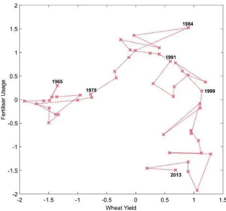
The subsequent recovery in EDI is driven by the decoupling of fertiliser usage and 216
yield, with wheat yields stable after 1984 despite a significant decline in fertiliser usage (in 217
particular of phosphate in arable areas) (Figure 3). This reflects improved farming practice in 218
the targeted application of fertiliser in response to new regulations such as the introduction of 219
Nitrate Vulnerable Zones in 1998-2002, knowledge exchange with academic and advisory 220
bodies (such as the Agriculture and Horticulture Development Board), and increasing 221
fertiliser prices (Firbank et al., 2011), as well as a reduction in cattle numbers and increased 222
Consequently, there is a reduction in the contamination of rivers by fertiliser runoff and a 224
decline in atmospheric emissions, aided by the rapid drop in livestock numbers in the 2000s 225
(partially due to the 2001 foot-and-mouth disease outbreak and subsidy reform) and the 226
banning of field burning in 1993. Stagnating yields have been linked to the growing impact of 227
climate extremes and changes in rotation practices (Brisson et al., 2010; Knight et al., 2012). 228
In contrast to the improvements in river and atmospheric pollution, farmland 229
biodiversity failed to recover after the initial rapid decline in the early 1980s despite 230
improvements in river nutrient contamination and atmospheric emissions. This suggests that 231
the drivers of farmland biodiversity decline are different from the drivers of river nutrient 232
contamination and atmospheric emissions, and have been hypothesised to be linked to factors 233
such as sowing timing, grassland improvement, habitat diversity, and livestock stocking 234
density (Benton et al., 2003; Butler et al., 2007; Chamberlain et al., 2000; Firbank et al., 2008; 235
Fuller, 2000; Krebs et al., 1999; Newton, 2004). A gradual increase in ‘land sparing’ in 236
England since 1950 (Supplementary Figure S5), potentially linked to intensification on 237
productive land making marginal land less economically viable and therefore more suitable 238
for ‘sparing’ for conservation purposes (Balmford et al., 2015, 2005; Ewers et al., 2009; 239
Green et al., 2005; Phalan et al., 2016), has not compensated for overall farmland biodiversity 240
decline. This may be due to sparing mostly taking place from rough grazing land in upland 241
regions and low-yielding common land rather than from more intensive arable or pastoral 242
lowland areas, and so has not directly benefited the wildlife specifically dependent on the 243
latter for which the FBI acts as a proxy for. However, the expansion of agri-environment 244
schemes such as aside land in the early 1990s and environmental stewardship after set-245
aside was discontinued in 2005 does coincide with a reduced rate of decline in the FBI 246
(DEFRA, 2015a). Farmland biodiversity is a key ecosystem service in the wider 247
agroecosystem, and its continued decline undermines the overall SI trend (Baulcombe et al., 248
English agroecosystem has not yet reached a safe operating space, and that novel approaches 250
to halting and reversing farmland biodiversity loss are required that are not included in the 251
current SI process. In contrast to the other indices, the extrapolated Soil Erosion Index shows 252
no discernible trend and only correlates with average yearly rainfall in the regional indices. 253
Socioeconomic trends for the English agroecosystem tend to not correlate with as 254
many variables as the biophysical variables in the correlation analysis (Table 2). Wheat yield 255
is strongly correlated with farm subsidies, which reflects increased direct subsidies to farmers 256
after 1992 coinciding with elevated yields, and does not imply causation. High farm income 257
and fertiliser usage correlate with higher intermediate consumption (i.e. total farm spending), 258
and high food prices correlate with lower livestock outputs. Total farm income appears to 259
partially follow trends in both Food Price Index and farm subsidies (Figure 1) but is not 260
significantly correlated with either. Despite a general increase in total farm income from a 261
minimum in 2000, by the end of our study period ~46% of UK farms failed to recover their 262
costs in that year and therefore remain heavily dependent on subsidies (DEFRA, 2015b). This 263
reliance on EU subsidies results in income fluctuations following the sterling-euro exchange 264
rate (e.g. the drop in subsidies in 2014 (DEFRA, 2015b)) and could lead to major changes in 265
income during and following the UK’s withdrawal from the EU (‘Brexit’). As a result, future 266
SI needs to incorporate the changing role of subsidies and ensure the financial security of 267
farmers. No directly causative correlations were found with farm labour headcount, with 268
continuously declining employment strongly anti-correlating with GDP per capita growth. 269
This decline reflects continued agricultural modernisation and mechanisation, with growing 270
national wealth associated with a peak and then a decline in the proportion of UK GDP and 271
labour force involved in agriculture. 272
These trends are also supported by both the DCA (Supplementary Figure S8) and PCA 273
(Supplementary Figure S9) results. Most of the data variance lies in the first axis (DCA1: 274
an initial state associated with lower yields, high inputs (including labour and fertiliser), high 276
river/atmosphere pollution (linked to inputs, e.g. high fertiliser use, and livestock), higher 277
income, lower subsidies and food prices, to a new state with higher yields, lower inputs and 278
river/atmosphere pollution, lower farm employment and income, and higher subsidies and 279
food prices. We interpret this as primarily reflecting both the modernisation and 280
commencement of sustainable intensification of English agriculture during the study time-281
period. There are also contributions to DCA1 and PC1 from increasing population, increasing 282
temperatures, and the continual deterioration of farmland biodiversity. DCA2 and PC2 283
explains much less of the data variance (DCA2: eigenvalue of 0.03905, axis length of 284
0.81272; PC2: ~16% of variance) and have differing contributions from each variable with no 285
obvious overall interpretation. DCA2 is notable though for the strong opposition of river 286
nutrient contamination versus rainfall and soil erosion, which could potentially arise from 287
high rainfall years being associated with diluted contamination but higher soil erosion. 288
3.2. Regional Differences 289
Regional Z-score time-series, PCA, DCA, and correlation analyses show that the 290
trends and correlations of the key variables of the Eastern England and South-Western 291
England agroecosystems are mostly similar to the all-England analyses, but that there are 292
some differences. In contrast to the all-England analysis, in our extrapolated soil erosion 293
index arable Eastern England experiences relatively high soil erosion rates during the 1980s 294
and early 1990s followed by a decline, while pastoral South-Western England appears to have 295
had overall increasing soil erosion rates since the early 1990s (Supplementary Figures S11 & 296
S15). Eastern England also experiences an earlier and higher peak in environmental 297
degradation before subsequently showing a stronger recovery than the rest of England, and 298
rainfall trends also do not correlate as well with other variables in Eastern England 299
all-England PCA results, with PC1 containing similar trends and accounting for ~62% and 301
~54% of the data variance in Eastern and South-Western England respectively, and PC2 302
explaining an additional ~14% and ~16% respectively (Supplementary Figures S12-S13 & 303
S16-S17). However, in Eastern England soil erosion increases with positive PC1 values 304
reflecting the gradual reduction in soil erosion over time in contrast to all-England, and PC2 305
also reflects higher rainfall and temperature along with higher atmospheric emissions, wheat 306
yield, and soil erosion in the negative direction. Eastern England differs more from all-307
England than South-Western England in all analyses, which along with the rainfall and soil 308
erosion trends we suggest is because most of England more closely resembles the mixed and 309
pastoral farming of South-Western England with higher rainfall and more variable topography 310
(falling in the larger Celtic broadleaf forest WWF ecoregion) than the intensive arable 311
agriculture concentrated in drier and lower-lying Eastern England (mostly falling in the 312
smaller English lowland beech forest WWF ecoregion) (Morton et al., 2011; Olson et al., 313
2001). Eastern England’s earlier and higher peak in environmental degradation implies the 314
rapid intensification of arable agriculture in this region had stronger impacts than in South-315
Western England, but that these impacts have now mostly abated. However, our analysis does 316
not include more novel impacts of intensive agriculture, such as recent evidence of potentially 317
harmful levels of riverine neonicotinoid (a controversial insecticide) contamination clustered 318
in Eastern England (Shardlow, 2017). 319
4. Environmental Kuznets Curves and Degradation ‘Offshoring’
320
Environmental degradation appears to follow the trajectory of an EKC in both the 321
whole English agroecosystem as well as in both Eastern and South-Western England. Both 322
wheat yield and degradation increase up to UK GDP per capita per annum of ~£17000 before 323
degradation declines with further increases in GDP while wheat yields stabilise (although 324
2). As a result, environmental degradation in the English agroecosystem partially follows a 326
classic EKC trajectory (Dinda, 2004), with soil, air, and water degradation (but not 327
biodiversity) rising with economic development before declining past a critical threshold as 328
more efficient technologies and practice (e.g. one-pass systems, new crop varieties, integrated 329
pest management (Baulcombe et al., 2009)) and environmental regulation (e.g. Nitrate 330
Vulnerable Zones) are established. The gap between falling environmental degradation and 331
stable yields relative to GDP (Figure 2) provides clear evidence that some degree of SI has 332
taken place, as yields have been maintained with a smaller environmental footprint whilst 333
overall prosperity has continued to grow. However, this overall trend is not reflected by 334
farmland biodiversity, which continues to decline despite economic growth and so displays no 335
Kuznets Curve behaviour itself. SI tends to be associated with greater resource use efficiency, 336
which can generate a cleaner environment but not necessarily a more biodiverse one (Firbank, 337
2005). Additionally, having increased to a peak in the early 1980s with intensification since 338
the mid-1990s UK agricultural self-sufficiency has declined from ~74% to ~60% for all food 339
(or ~85% to below 75% for just indigenous-type food) (DEFRA, 2016b), indicating that some 340
of the UK’s agricultural impact has effectively been offshored to other agroecosystems as a 341
result of globalisation (Figure 1 & Supplementary Figure S6). This implies that environmental 342
degradation may not have declined so much or at all if the UK had maintained or increased 343
self-sufficiency in food production between 1980 and 2013. Together with poor biodiversity 344
trends, this indicates that only partial SI has been achieved in the UK in this time, and that in 345
order to reach both regional and global safe operating spaces for agroecosystems future SI 346
will need to both halt biodiversity loss and ensure damaging practices are not simply 347
offshored to poorer countries with weaker regulations. On the regional scale, degradation in 348
South-Western England matches the trajectory of all-England fairly closely (despite an 349
apparent resurgence in EDI in 2006 due to anomalously and potentially unreliably high 350
England occurs more rapidly and then subsequently improves by a greater degree than South-352
Western or all-England. This further illustrates the greater and more rapid impact on the 353
environment of arable intensification versus the intensification of mixed or pastoral farming 354
elsewhere. 355
5. Conceptual Modelling
356
5.1. Model Development 357
Following the data analysis we developed a simple system dynamics model using the 358
Vensim PLE platform (Ventana Systems Inc., 2015) in order to further evaluate our 359
understanding of the relationships within the English agroecosystem and the impacts of the 360
changing nature of intensification between 1980 and 2013. Simple system dynamics models 361
are a useful way to rapidly explore our understanding of a dynamical system using relative 362
trends rather than absolute quantities (e.g. Meadows, 2008; Meadows et al., 1972). We 363
restricted the relationships in the model to those that are both: a) commonly proposed as 364
causative in the literature and from expert judgement, and b) showed statistically significant 365
correlations in our dataset (Table 2 & Supplementary Figure S10), in order to exclude 366
spurious correlations. We use simple linear relationships and approximated trends of fertiliser 367
usage, livestock population, temperature, rainfall, farm subsidy, and farm income in order to 368
drive changes in farm biodiversity, yield, atmospheric emissions, soil erosion, river nutrient 369
contamination, and input spending for the 1980-2013 period (Figure 4). Each variable 370
changes according to the averaged changes of its input variables – for example, changes in 371
River Nutrient Contamination are the average of the changes in Fertiliser Usage, Livestock, 372
and Rainfall – and assumes equal weighting for each input. This assumption is likely to be 373
inaccurate as some factors will be more important than others, but in the absence of further 374
from this model which we exclude due to a lack of full datasets or direct correlations, such as 376
level of mechanisation and food prices. There are no closed loops in this model, and so no 377
feedback loops are expected to operate. 378
The model successfully recreates the trends in the non-driver variables for this time 379
period (Figure 1 & Figure 4), with yield increasing and then plateauing, farm biodiversity 380
declining and then plateauing, both river nutrient contamination and atmospheric emissions 381
peaking and then declining as fertiliser use and livestock populations peak, soil erosion 382
staying fairly level in the long-term, and input spending dropping in the 1990s. Yield is 383
dependent on a normative ‘Sustainable Intensification’ variable that we introduce, which has 384
to constantly increase in order to offset the impact of declining fertiliser usage. In this context 385
SI represents improved fertiliser application practices and other improvements in crop 386
management, but is not represented by a direct data proxy in our analysis and so has an 387
imposed linear increase over time. Removing this SI variable results in yield peaking and then 388
declining in line with fertiliser usage. 389
5.2. Future Projections 390
In order to use the system dynamics model for future scenario exploration further 391
hypothetical relationships that are likely to play a role in affecting future trends are added to 392
the model (shown by the red arrows and variables in Figure 5 and based on the possibly 393
linked causal relationships in Table 2) and projected trends for model drivers imposed, 394
including consistently increasing temperature, an erratic rainfall trend, stable subsidies 395
(uncertain in a post-Brexit context), and stable but high food prices (Figure 5). While mean 396
annual temperature and yield are positively correlated in our data between 1980 and 2013, it 397
is likely that further temperature increases will begin to reverse this correlation in the future 398
and so we model further temperature increases to have net negative impacts on yields. We 399
not available, for which we have estimated their past long-term trends. Based on this we 401
explore several future scenarios featuring different responses to exogenous forcing such as 402
increasing temperature and increasing variance in rainfall (Figure 5). 403
In the ‘Continual SI’ scenario we allow SI to improve at a constant rate (increasing by 404
a further 112% more than the 1980-2013 improvement), which counteracts the negative 405
impact of increasing temperature, stabilises biodiversity loss, and reduces soil erosion despite 406
consistent levels of mechanisation. If SI is instead kept fixed at 2013 levels until 2050 (‘No 407
Further SI’ scenario), yields begin to fall and improvements are not observed after 2013 in the 408
latter variables. In order to allow biodiversity to gradually recover while yield remains stable 409
(‘Biodiverse SI’ scenario) it is necessary to reduce mechanisation and pesticide use to ~73% 410
and ~20% below 2013 levels respectively while significantly increasing SI (to 200% more 411
than the 1980-2013 improvement). Increasing yield beyond current levels rather than allowing 412
it to plateau indefinitely (‘Maximise Yield’ scenario) requires some combination of this 413
accelerated SI and increased mechanisation (by 75%), fertiliser usage (to previous peak), or 414
pesticide use (to previous peak), but increasing these latter variables also reverses the 415
recovery in fertiliser pollution and forces biodiversity into dangerous decline. Allowing a 416
gradual recovery in livestock population to previous peak levels in conjunction with 417
‘Continual SI’ (‘Livestock Intensification’ scenario) results in partial reversals to the 418
recoveries in atmospheric emissions and river nutrient contamination, although neither 419
reaches the levels seen in the 1980s unless fertiliser use also increases. 420
These results suggest that it is difficult to both increase yield or livestock population 421
and limit environmental degradation and further biodiversity decline without continual and 422
significant improvements in SI. However, the SI variable is a significant simplification of a 423
complex set of decisions, processes, and impacts surrounding farming practice with no upper 424
limits, and it cannot be assumed that SI can consistently increase in order to offset other 425
dynamics is needed. 427
6. Conclusions
428
In this study we use publicly available data to construct metrics assessing the impact 429
of agricultural intensification on environmental degradation in the English agroecosystem and 430
use a simple system dynamics model to analyse future scenarios. From these analyses it is 431
clear that agricultural intensification drove increased environmental degradation in England 432
during the 1980s. In the 1990s fertiliser and pesticide usage decoupled from high yields with a 433
reversal in the degradation of several ecosystem services (e.g. river nutrient contamination 434
and atmospheric emissions), suggesting that SI began to take place. When plotted against 435
GDP per capita this process follows an Environmental Kuznets Curve, suggesting better 436
environmental protection with greater prosperity. Despite an increase in land sparing, 437
farmland biodiversity has not experienced any recovery making it the major negative trade-off 438
in current SI practices. Additionally, reduced agricultural self-sufficiency indicates some 439
agricultural impacts may have been ‘offshored’ abroad. These two outcomes undermine 440
attempts to achieve future English and global SI and indicate that English agroecosystems 441
have not yet reached a safe or just operating space. Similar patterns are observed in both 442
arable-dominated Eastern England and pastoral-dominated South-Western England, although 443
the impact of intensification was stronger in arable Eastern England. A simple system 444
dynamics model of the English agroecosystem recreates the basic trends of several ecosystem 445
services between 1980 and 2013 when assuming an increase in SI. The impacts of uncertain 446
levels of subsidies post-Brexit and increasing climatic impacts were explored in future 447
scenarios. These show that: maintaining or increasing yields and livestock populations while 448
also restoring biodiversity; maintaining the environmental gains achieved since the 1990s; and 449
improving the financial viability of farming, will all prove challenging. Further SI featuring 450
agri-environment schemes focusing on restoring biodiversity and reducing degradation 452
offshoring – is required to meet these challenges, but the extent to which further 453
Acknowledgements
455
This work was supported by the Research Stimulus Fund of the Institute for Life Sciences at 456
the University of Southampton. We are grateful to FERA PUS Stats and in particular David 457
Garthwaite for providing an as-of-yet unpublished extension to their pesticide usage datasets. 458
Author Contributions
459
All authors designed the research; DIAM performed the data analysis and modelling; all 460
authors contributed to the interpretation of the data analysis and modelling results; DIAM 461
wrote the paper with input from all other authors; all authors gave final approval for 462
publication. 463
Competing Interests
464
The authors declare no competing interests. 465
Data Availability
466
All data used in this study is available from publically accessible data sources cited in the text 467
(see Table 1 for sources), with the minor exception of an as-of-yet unpublished extension to 468
the pesticide usage dataset (provided on request by David Garthwaite and FERA PUS Stats) 469
which provides critical extra context to the peak and decline of pesticide use in the UK. 470
References
472
Balmford, A., Green, R., Phalan, B., 2015. Land for Food & Land for Nature? Daedalus 144, 473
57–75. https://doi.org/10.1162/DAED_a_00354 474
Balmford, A., Green, R.E., Scharlemann, J.P.W., 2005. Sparing land for nature: exploring the 475
potential impact of changes in agricultural yield on the area needed for crop production. 476
Glob. Chang. Biol. 11, 1594–1605. 477
Baulcombe, D., Crute, I., Davies, B., Dunwell, J., Gale, M., Jones, J., Pretty, J., Sutherland, 478
W., Toulmin, C., 2009. Reaping the benefits: science and the sustainable intensification 479
of global agriculture. 480
Benton, T.G., Bryant, D.M., Cole, L., Crick, H.Q.P., 2002. Linking agricultural practice to 481
insect and bird populations: A historical study over three decades. J. Appl. Ecol. 39, 673– 482
687. https://doi.org/10.1046/j.1365-2664.2002.00745.x 483
Benton, T.G., Vickery, J.A., Wilson, J.D., 2003. Farmland biodiversity: Is habitat 484
heterogeneity the key? Trends Ecol. Evol. 18, 182–188. https://doi.org/10.1016/S0169-485
5347(03)00011-9 486
Boardman, J., 2013. Soil Erosion in Britain: Updating the Record. Agriculture 3, 418–442. 487
https://doi.org/10.3390/agriculture3030418 488
Brisson, N., Gate, P., Gouache, D., Charmet, G., Oury, F.X., Huard, F., 2010. Why are wheat 489
yields stagnating in Europe? A comprehensive data analysis for France. F. Crop. Res. 490
119, 201–212. https://doi.org/10.1016/j.fcr.2010.07.012 491
Butler, S.J., Vickery, J.A., Norris, K., 2007. Farmland Biodiversity and the Footprint of 492
Agriculture. Science. 315, 381–384. https://doi.org/10.1126/science.1136607 493
Carpenter, S.R., Mooney, H.A., Agard, J., Capistrano, D., DeFries, R.S., Diaz, S., Dietz, T., 494
Duraiappah, A.K., Oteng-Yeboah, A., Pereira, H.M., Perrings, C., Reid, W. V., Sarukhan, 495
J., Scholes, R.J., Whyte, A., 2009. Science for managing ecosystem services: Beyond the 496
Millennium Ecosystem Assessment. Proc. Natl. Acad. Sci. 106, 1305–1312. 497
https://doi.org/10.1073/pnas.0808772106 498
Chamberlain, E.E., Fuller, R.J., Bunce, R.G.H., Duckworth, J.C., Shrubb, M., 2000. Changes 499
in the abundance of farmland birds in relation to the timing of agricultural intensifcation 500
in England and Wales. J. Appl. Ecol. 501
Dearing, J.A., Wang, R., Zhang, K., Dyke, J.G., Haberl, H., Hossain, M.S., Langdon, P.G., 502
Lenton, T.M., Raworth, K., Brown, S., Carstensen, J., Cole, M.J., Cornell, S.E., Dawson, 503
T.P., Doncaster, C.P., Eigenbrod, F., Flörke, M., Jeffers, E., Mackay, A.W., Nykvist, B., 504
Poppy, G.M., 2014. Safe and just operating spaces for regional social-ecological systems. 505
Glob. Environ. Chang. 28, 227–238. https://doi.org/10.1016/j.gloenvcha.2014.06.012 506
Dearing, J.A., Yang, X., Dong, X., Zhang, E., Chen, X., Langdon, P.G., Zhang, K., Zhang, W., 507
Dawson, T.P., 2012. Extending the timescale and range of ecosystem services through 508
paleoenvironmental analyses, exemplified in the lower Yangtze basin. Proc. Natl. Acad. 509
Sci. 109, E1111–E1120. https://doi.org/10.1073/pnas.1118263109 510
DEFRA, 2016a. UK biodiversity indicators 2015: Measuring progress towards halting 511
biodiversity loss. 512
DEFRA, 2016b. Overseas trade in food, feed and drink [WWW Document]. URL 513
https://www.gov.uk/government/statistical-data-sets/overseas-trade-in-food-feed-and-514
DEFRA, 2015a. Agri-environment indicators [WWW Document]. URL 516 https://www.gov.uk/government/statistical-data-sets/agri-environment-indicators 517 (accessed 10.14.15). 518
DEFRA, 2015b. Agriculture in the United Kingdom 2014. 519
DEFRA, 2015c. Total income from farming in the UK [WWW Document]. URL 520
https://www.gov.uk/government/statistics/total-income-from-farming-in-the-uk (accessed 521
5.23.16). 522
DEFRA, 2014a. The British Survey of Fertiliser Practice: Fertiliser Use on Farm Crops for 523
Crop Year 2013. 524
DEFRA, 2014b. Cereal Production Survey [WWW Document]. URL 525
https://data.gov.uk/dataset/cereals_and_oilseeds_production_harvest (accessed 5.23.16). 526
DEFRA, 2014c. June Survey of Agriculture and Horticulture, UK [WWW Document]. URL 527
https://data.gov.uk/dataset/june_survey_of_agriculture_and_horticulture_uk (accessed 528
9.1.15). 529
Dinda, S., 2004. Environmental Kuznets Curve Hypothesis: A Survey. Ecol. Econ. 49, 431– 530
455. https://doi.org/10.1016/j.ecolecon.2004.02.011 531
Environment Agency, 2014. Historic UK Water Quality Sampling Harmonised Monitoring 532
Scheme Summary Data [WWW Document]. URL https://data.gov.uk/dataset/historic-uk-533
water-quality-sampling-harmonised-monitoring-scheme-summary-data (accessed 534
1.14.16). 535
Ewers, R.M., Scharlemann, J.P.W., Balmford, A., Green, R.E., 2009. Do increases in 536
agricultural yield spare land for nature? Glob. Chang. Biol. 15, 1716–1726. 537
https://doi.org/10.1111/j.1365-2486.2009.01849.x 538
FERA PUS Stats, 2015. Pesticide Usage Survey [WWW Document]. URL 539
https://secure.fera.defra.gov.uk/pusstats/index.cfm (accessed 10.14.15). 540
Firbank, L., Bradbury, R., McCracken, D., Stoate, C., Goulding, K., Harmer, R., Hess, T., 541
Jenkins, A., Pilgrim, E., Potts, S., Smith, P., Ragab, R., Storkey, J., Williams, P., 2011. 542
Enclosed farmland, in: UK National Ecosystem Assessment: Technical Report. UNEP-543
WCMC, Cambridge, UK, pp. 197–240. 544
Firbank, L.G., 2005. Striking the balance between agricultural production and biodiversity. 545
Ann. Appl. Biol. 146, 163–175. https://doi.org/citeulike-article-id:6126868 546
Firbank, L.G., Bradbury, R.B., McCracken, D.I., Stoate, C., 2013a. Delivering multiple 547
ecosystem services from Enclosed Farmland in the UK. Agric. Ecosyst. Environ. 166, 548
65–75. https://doi.org/10.1016/j.agee.2011.11.014 549
Firbank, L.G., Elliott, J., Drake, B., Cao, Y., Gooday, R., 2013b. Evidence of sustainable 550
intensification among British farms. Agric. Ecosyst. Environ. 173, 58–65. 551
https://doi.org/10.1016/j.agee.2013.04.010 552
Firbank, L.G., Petit, S., Smart, S., Blain, A., Fuller, R.J., 2008. Assessing the impacts of 553
agricultural intensification on biodiversity: a British perspective. Philos. Trans. R. Soc. B 554
Biol. Sci. 363, 777–787. https://doi.org/10.1098/rstb.2007.2183 555
Fuller, R., 2000. Relationships between recent changes in lowland British agriculture and 556
farmland bird populations: an overview. Ecol. Conserv. Lowl. Farml. birds. Proc. 1999 557
BOU Spring Conf. 1950, 5–16. 558
Garnett, T., Appleby, M.C., Balmford, A., Bateman, I.J., Benton, T.G., Bloomer, P., 559
P., Thornton, P.K., Toulmin, C., Vermeulen, S.J., Godfray, H.C.J., 2013. Sustainable 561
Intensification in Agriculture: Premises and Policies. Science. 341, 33–34. 562
https://doi.org/10.1126/science.1234485 563
Garthwaite, D., Unpublished. Data: Historical Pesticide Usage on Arable Crops. 564
Godfray, C.H.J., Garnett, T., 2014. Food security and sustainable intensification. Philos. 565
Trans. R. Soc. 369, 6–11. 566
Great Britain Historical GIS Project, 2015. A Vision of Britain Through Time: Census Reports 567
[WWW Document]. URL http://www.visionofbritain.org.uk/census/ (accessed 10.12.15). 568
Green, R.E., Cornell, S.J., Scharlemann, J.P.W., Balmford, A., 2005. Farming and the Fate of 569
Wild Nature. Science. 307, 550–555. https://doi.org/10.1126/science.1106049 570
Grossman, G.M., Krueger, A.B., 1995. Economic Growth and the Environment Author. Q. J. 571
Econ. 110, 353–377. 572
Hawkesford, M.J., 2014. Reducing the reliance on nitrogen fertilizer for wheat production. J. 573
Cereal Sci. 59, 276–283. https://doi.org/10.1016/j.jcs.2013.12.001 574
Hayhow, D., Eaton, M., Gregory, R., Burns, F., 2016. State of Nature 2016 1–87. 575
Jones, P.D., Lister, D.H., Kostopoulou, E., 2004. Reconstructed river flow series from 1860s 576
to present (Science Report SC040052/SR). 577
Knight, S., Kightley, S., Bingham, I., Hoad, S., Lang, B., Philpott, H., Stobart, R., Thomas, J., 578
Barnes, A., Ball, B., 2012. “Yield Plateau” in Wheat and Oilseed Rape. 579
Krebs, J.R., Wilson, J.D., Bradbury, R.B., Siriwardena, G.M., 1999. The second Silent 580
Spring? Nature 400, 611–612. https://doi.org/10.1038/23127 581
Lindenmayer, D.B., Likens, G.E., 2011. Direct Measurement Versus Surrogate Indicator 582
Species for Evaluating Environmental Change and Biodiversity Loss. Ecosystems 14, 583
47–59. https://doi.org/10.1007/s10021-010-9394-6 584
Loos, J., Abson, D.J., Chappell, M.J., Hanspach, J., Mikulcak, F., Tichit, M., Fischer, J., 2014. 585
Putting meaning back into “sustainable intensification.” Front. Ecol. Environ. 12, 356– 586
361. https://doi.org/10.1890/130157 587
Mace, G.M., Norris, K., Fitter, A.H., 2012. Biodiversity and ecosystem services: A 588
multilayered relationship. Trends Ecol. Evol. 27, 19–25. 589
https://doi.org/10.1016/j.tree.2011.08.006 590
MacFadyen, S., Gibson, R., Polaszek, A., Morris, R.J., Craze, P.G., Planqué, R., Symondson, 591
W.O.C., Memmott, J., 2009. Do differences in food web structure between organic and 592
conventional farms affect the ecosystem service of pest control? Ecol. Lett. 12, 229–238. 593
https://doi.org/10.1111/j.1461-0248.2008.01279.x 594
Mahon, N., Crute, I., Simmons, E., Islam, M.M., 2017. Sustainable intensification – 595
“oxymoron” or “third-way”? A systematic review. Ecol. Indic. 74, 73–97. 596
https://doi.org/10.1016/j.ecolind.2016.11.001 597
Maron, M., Lill, A., 2005. The influence of livestock grazing and weed invasion on habitat 598
use by birds in grassy woodland remnants. Biol. Conserv. 124, 439–450. 599
https://doi.org/10.1016/j.biocon.2005.02.002 600
Mathews, F., Kubasiewicz, L., Gurnell, J., Harrower, C., McDonald, R., Shore, R., 2018. A 601
Review of the Population and Conservation Status of British Mammals: Technical 602
Summary. A report by the Mammal Society under contract to Natural England, Natural 603
Meadows, D.H., 2008. Thinking in Systems: A Primer. Chelsea Green Publishing, White 605
River Junction, Vermont. 606
Meadows, D.H., Meadows, D., Randers, J., Behrens III, W.W., 1972. The Limits to Growth: A 607
Report for the Club of Rome’s Project on the Predicament of Mankind. Universe Books, 608
New York. 609
Met Office, 2015. UK and regional series [WWW Document]. URL 610
http://www.metoffice.gov.uk/climate/uk/summaries/datasets (accessed 1.15.16). 611
Millennium Ecosystem Assessment, 2005. Ecosystems and Human Well-being: Synthesis. 612
Island Press, Washington DC. 613
Morton, D., Rowland, C., Wood, C., Meek, L., Marston, C., Smith, G., Wadsworth, R., 614
Simpson, I.C., 2011. Countryside Survey: Final Report for LCM2007 - the new UK Land 615
Cover Map. 616
Natural Capital Committee, 2017. How to do it: a natural capital workbook. Version 1. 617
Newton, I., 2004. The recent declines of farmland bird populations in Britain: an appraisal of 618
causal factors and conservation actions. Ibis (Lond. 1859). 146, 579–600. 619
https://doi.org/10.1111/j.1474-919X.2004.00375.x 620
Oksanen, J., Blanchet, F.G., Friendly, M., Kindt, R., Legendre, P., McGlinn, D., Minchin, 621
P.R., O’Hara, R.B., Simpson, G.L., Solymos, P., Stevens, M.H.H., Szoecs, E., Wagner, 622
H., 2017. vegan: Community Ecology Package. 623
Olson, D.M., Dinerstein, E., Wikramanayake, E.D., Burgess, N.D., Powell, G.V.N., 624
Underwood, E.C., D’amico, J. a., Itoua, I., Strand, H.E., Morrison, J.C., Loucks, C.J., 625
Allnutt, T.F., Ricketts, T.H., Kura, Y., Lamoreux, J.F., Wettengel, W.W., Hedao, P., 626
Kassem, K.R., 2001. Terrestrial Ecoregions of the World: A New Map of Life on Earth. 627
Bioscience 51, 933. https://doi.org/10.1641/0006-3568 628
ONS, 2015a. Office for National Statistics: Population estimates [WWW Document]. URL 629
https://www.ons.gov.uk/peoplepopulationandcommunity/populationandmigration/popula 630
tionestimates (accessed 10.13.15). 631
ONS, 2015b. United Kingdom Economic Accounts: Gross Domestic Product (GDP) [WWW 632
Document]. URL https://www.ons.gov.uk/economy/grossdomesticproductgdp#timeseries 633
(accessed 12.17.15). 634
Peterson, B.G., Carl, P., 2014. PerformanceAnalytics: Econometric tools for performance and 635
risk analysis. 636
Phalan, B., Green, R.E., Dicks, L. V., Dotta, G., Feniuk, C., Lamb, A., Strassburg, B.B.N., 637
Williams, D.R., Ermgassen, E.K.H.J. z., Balmford, A., 2016. How can higher-yield 638
farming help to spare nature? Science. 351, 450–451. 639
https://doi.org/10.1126/science.aad0055 640
Poppy, G.M., Chiotha, S., Eigenbrod, F., Harvey, C. a, Honzak, M., Hudson, M.D., Jarvis, A., 641
Madise, N.J., Schreckenberg, K., Shackleton, C.M., Villa, F., Dawson, T.P., 2014a. Food 642
security in a perfect storm: using the ecosystem services framework to increase 643
understanding. Philos. Trans. R. Soc. B Biol. Sci. 369, 20120288–20120288. 644
https://doi.org/10.1098/rstb.2012.0288 645
Poppy, G.M., Jepson, P.C., Pickett, J.A., Birkett, M.A., 2014b. Achieving food and 646
environmental security: new approaches to close the gap. Philos. Trans. R. Soc. Lond. B. 647
Biol. Sci. 369, 20120272. https://doi.org/10.1098/rstb.2012.0272 648
Pretty, J.N., 1997. The sustainable intensification of agriculture. Nat. Resour. Forum 21, 247– 649
R Foundation for Statistical Computing, 2016. R: A language and environment for statistical 651
computing. 652
Razeng, E., Watson, D.M., 2015. Nutritional composition of the preferred prey of 653
insectivorous birds: popularity reflects quality. J. Avian Biol. 46, 89–96. 654
https://doi.org/10.1111/jav.00475 655
Razeng, E., Watson, D.M., 2010. What do declining woodland birds eat? A synthesis of 656
dietary records. Emu. https://doi.org/doi.org/10.1071/MU11099 657
Rockström, J., Steffen, W., Noone, K., Persson, Å., Chapin, F.S., Lambin, E.F., Lenton, T.M., 658
Scheffer, M., Folke, C., Schellnhuber, H.J., Nykvist, B., de Wit, C.A., Hughes, T., van 659
der Leeuw, S., Rodhe, H., Sörlin, S., Snyder, P.K., Costanza, R., Svedin, U., Falkenmark, 660
M., Karlberg, L., Corell, R.W., Fabry, V.J., Hansen, J., Walker, B., Liverman, D., 661
Richardson, K., Crutzen, P., Foley, J.A., 2009. A safe operating space for humanity. 662
Nature 461, 472–475. https://doi.org/10.1038/461472a 663
Rockström, J., Williams, J., Daily, G., Noble, A., Matthews, N., Gordon, L., Wetterstrand, H., 664
DeClerck, F., Shah, M., Steduto, P., de Fraiture, C., Hatibu, N., Unver, O., Bird, J., 665
Sibanda, L., Smith, J., 2017. Sustainable intensification of agriculture for human 666
prosperity and global sustainability. Ambio 46, 4–17. https://doi.org/10.1007/s13280-667
016-0793-6 668
Salisbury, E., Thistlethwaite, G., Pang, Y., Misra, A., 2015. Air Quality Pollutant Inventories 669
for England, Scotland, Wales and Northern Ireland: 1990-2013. 670
Shardlow, M., 2017. Neonicotinoid Insecticides in British Freshwaters: 2016 Water 671
Framework Directive Watch List Monitoring Results and Recommendations. 672
Peterborough. 673
Srivastava, D.S., Vellend, M., 2005. Biodiversity-Ecosystem Function Research : Is It 674
Relevant to Conservation? Annu. Rev. Ecol. Evol. Syst. 36, 267–294. 675
Steffen, W., Broadgate, W., Deutsch, L., Gaffney, O., Ludwig, C., 2015. The trajectory of the 676
Anthropocene: The Great Acceleration. Anthr. Rev. 2, 81–98. 677
https://doi.org/10.1177/2053019614564785 678
The MathWorks Inc., 2016. Matlab Release 2016a. 679
Thiaw, I., Kumar, P., Yashiro, M., Molinero, C., 2011. Food and Ecological Security: 680
Identifying synergy and trade-offs, UNEP Policy Series. 681
Tilman, D., Balzer, C., Hill, J., Befort, B.L., 2011. Global food demand and the sustainable 682
intensification of agriculture. Proc. Natl. Acad. Sci. 1–5. 683
https://doi.org/10.1073/pnas.1116437108 684
Tilman, D., Fargione, J., Wolff, B., D’Antonio, C., Dobson, A., Howarth, R., Schindler, D., 685
Schlesinger, W.H., Simberloff, D., Swackhamer, D., 2001. Forecasting Agriculturally 686
Driven Global Environmental Change. Science. 292, 281–284. 687
https://doi.org/10.1126/science.1057544 688
UN FAO, 2015. FAO Food Price Index [WWW Document]. URL 689
http://www.fao.org/worldfoodsituation/foodpricesindex/en/ (accessed 10.13.15). 690
UN Population Division, 2017. World Population Prospects: The 2017 Revision, Key 691
Findings and Advance Tables (No. ESA/P/WP/248). 692
Ventana Systems Inc., 2015. Vensim PLE. 693
Vitousek, P.M., Mooney, H.A., Lubchenco, J., Melillo, J.M., 1997. Human Domination of 694
https://doi.org/10.1126/science.277.5325.494 696
Zhang, K., Dearing, J.A., Dawson, T.P., Dong, X., Yang, X., Zhang, W., 2015. Poverty 697
alleviation strategies in eastern China lead to critical ecological dynamics. Sci. Total 698
Environ. 506–507, 164–181. https://doi.org/10.1016/j.scitotenv.2014.10.096 699
Figures and Tables
701
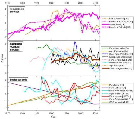
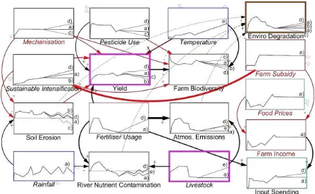
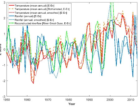
702
Figure 1: Z-score plot illustrating the evolution of the English agroecosystem as 703
reflected by indices of: a) provisioning ecosystem services, b) regulating/cultural ecosystem 704
services, and c) socioeconomic parameters. Climate data and regional variations are illustrated 705
707
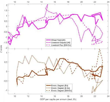
Figure 2: Phase plots of provisioning services (top) and the environmental degradation 708
index (bottom) in England and the sub-regions of Eastern and South-Western England versus 709
711
Figure 3: Phase plot of the Z-scores for wheat yield (UK) and fertiliser usage (total for 712
714
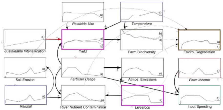
Figure 4: Simple system dynamics model for the English agroecosystem, with 715
simulation drivers/results for 1980-2013 shown in each variable box (italics for imposed 716
drivers). Scenarios include: a) with (blue lines) and b) without (red) SI. Arrow thickness 717
indicates correlation strength, dotted arrows show drivers of the Environmental Degradation 718
Index, the dashed arrow shows the hypothesised effect of Sustainable Intensification), arrow 719
symbols indicate correlation type (positive [+], negative [-], or variable [x]), and box colours 720
match the colours used in the Z-score plots (Figure 1; thick-lined boxes match thicker Z-score 721
723
Figure 5: Extended simple system dynamics model for the English agroecosystem, with 724
simulation drivers/results for 1980-2050 in different scenarios. Scenarios include: a) 725
‘Continual SI’ (blue lines), b) ‘No Further SI’ (black), c) ‘Biodiverse SI’ (grey), d) ‘Maximise 726
Yield’ (green), and e) ‘Livestock Intensification’ (red). Arrow and box weights and symbols 727
are as in Figure 4, except red text which indicates variables not included in the 1980-2013 728
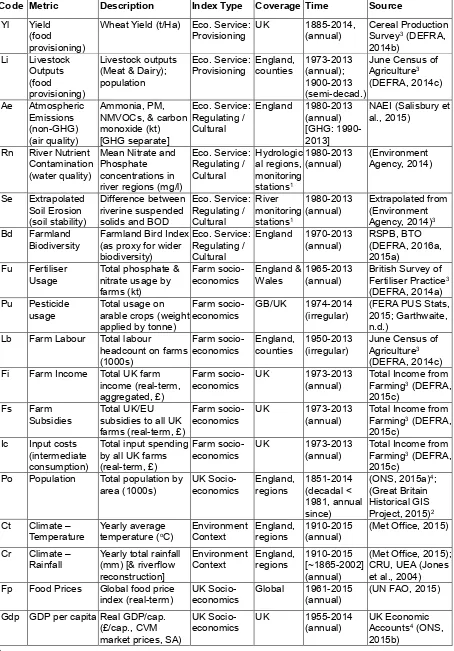
Table 1: Study datasets, including description, data type, data coverage, time period, 730
and data source. 731
Code Metric Description Index Type Coverage Time Source
Yl Yield (food provisioning)
Wheat Yield (t/Ha) Eco. Service:
Provisioning UK 1885-2014, (annual) Cereal Production Survey3 (DEFRA,
2014b) Li Livestock Outputs (food provisioning) Livestock outputs (Meat & Dairy); population
Eco. Service:
Provisioning England, counties 1973-2013 (annual); 1900-2013 (semi-decad.)
June Census of Agriculture3 (DEFRA, 2014c) Ae Atmospheric Emissions (non-GHG) (air quality) Ammonia, PM, NMVOCs, & carbon monoxide (kt) [GHG separate] Eco. Service: Regulating / Cultural England 1980-2013 (annual) [GHG: 1990-2013]
NAEI (Salisbury et al., 2015)
Rn River Nutrient Contamination (water quality)
Mean Nitrate and Phosphate concentrations in river regions (mg/l)
Eco. Service: Regulating / Cultural Hydrologic al regions, monitoring stations1 1980-2013
(annual) (Environment Agency, 2014)
Se Extrapolated Soil Erosion (soil stability)
Difference between riverine suspended solids and BOD
Eco. Service: Regulating / Cultural River monitoring stations1 1980-2013
(annual) Extrapolated from (Environment Agency, 2014)3
Bd Farmland
Biodiversity Farmland Bird Index (as proxy for wider biodiversity)
Eco. Service: Regulating / Cultural
England 1970-2013
(annual) RSPB, BTO (DEFRA, 2016a, 2015a)
Fu Fertiliser
Usage Total phosphate & nitrate usage by farms (kt)
Farm
socio-economics England & Wales 1965-2013 (annual) British Survey of Fertiliser Practice3
(DEFRA, 2014a) Pu Pesticide
usage Total usage on arable crops (weight applied by tonne)
Farm
socio-economics GB/UK 1974-2014 (irregular) (FERA PUS Stats, 2015; Garthwaite, n.d.)
Lb Farm Labour Total labour
headcount on farms (1000s)
Farm
socio-economics England, counties 1950-2013 (irregular) June Census of Agriculture3
(DEFRA, 2014c) Fi Farm Income Total UK farm
income (real-term, aggregated, £)
Farm
socio-economics UK 1973-2013 (annual) Total Income from Farming3 (DEFRA,
2015c) Fs Farm
Subsidies Total UK/EU subsidies to all UK farms (real-term, £)
Farm
socio-economics UK 1973-2013 (annual) Total Income from Farming3 (DEFRA,
2015c) Ic Input costs
(intermediate consumption)
Total input spending by all UK farms (real-term, £)
Farm
socio-economics UK 1973-2013 (annual) Total Income from Farming3 (DEFRA,
2015c) Po Population Total population by
area (1000s) UK Socio-economics England, regions 1851-2014 (decadal < 1981, annual since)
(ONS, 2015a)4;
(Great Britain Historical GIS Project, 2015)2
Ct Climate –
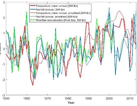
Temperature Yearly average temperature (oC) Environment Context England, regions 1910-2015 (annual) (Met Office, 2015)
Cr Climate –
Rainfall Yearly total rainfall (mm) [& riverflow reconstruction]
Environment
Context England, regions 1910-2015 [~1865-2002] (annual)
(Met Office, 2015); CRU, UEA (Jones et al., 2004) Fp Food Prices Global food price
index (real-term) UK Socio-economics Global 1961-2015 (annual) (UN FAO, 2015) Gdp GDP per capitaReal GDP/cap.
(£/cap., CVM market prices, SA)
UK
Socio-economics UK 1955-2014 (annual) UK Economic Accounts4 (ONS,
2015b)
1Hydrological Region stations: Anglian: Bedford Ouse; SW: Exe (plus Tamar for England average); SE: Medway
& Thames; Midlands: Severn & Trent; NE: Aire, Don, Tees, & Tyne; NW: Dee, Mersey, & Ribble 733
2This data is provided through www.VisionofBritain.org.uk and uses statistical material which is copyright of the
734
Great Britain Historical GIS Project, Humphrey Southall and the University of Portsmouth 735
3Crown copyright 2017. Adapted from data from the Department for Environment, Food and Rural Affairs under
736
the Open Government Licence v.3.0 (http://www.nationalarchives.gov.uk/doc/open-government-737
licence/version/3/). 738
4Crown copyright 2017. Adapted from data from the Office for National Statistics licensed under the Open
739
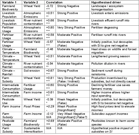
Table 2: Correlated variables from our correlation analysis hypothesised to represent 741
causal relationships (or only possibly linked in italics) in the English agroecosystem and used 742
to build the conceptual models. Correlation significance (p-value) is given as *** for p<0.001, 743
** for p<0.01, * for p<0.05, - for p<0.1, and N/A for p>0.1. 744
Variable 1 Variable 2 Correlation Hypothesised driver
Farmland
Biodiversity Wheat Yield -0.72*** Strong Negative Landscape / ecosystem homogenisation Livestock
Population Atmospheric Emissions +0.51** Strong Positive Livestock enteric emissions Livestock
Population River nutrient contamination +0.66*** Strong Positive Livestock effluent runoff into rivers Fertiliser
Usage Atmospheric Emissions +0.80*** Very Strong Positive Fertiliser degassing Fertiliser
Usage River nutrient contamination +0.58*** Moderate Positive Fertiliser runoff into rivers Fertiliser
Usage Wheat Yield -0.57*** Moderate Negative(False) Initially positive, but decouples with SI to give net negative Climate –
Temperature Farmland Biodiversity -0.46** Moderate Negative Heat stress on wildlife and forced migration Climate –
Temperature Wheat Yield +0.51** Moderate Positive Lengthened growing season Climate –
Rainfall River nutrient contamination -0.54** Moderate Negative Pollution dilution in rivers Climate –
Rainfall Soil erosion +0.67*** Strong Positive Sediment runoff during rainstorms Farm
Subsidy Wheat Yield +0.81*** Very Strong Positive (False / Indirect) Production incentivised by subsidies, but not directly causal Intermediate
Consumption Fertiliser Usage +0.60*** Strong Positive Declining fertiliser use saves farmers’ money Intermediate
Consumption Farm income +0.61*** Strong Positive Higher income allows higher input spending Pesticide
Use Wheat Yield -0.39* Weak Negative(False) Initially positive, but decouples with SI to become net negative
Farm Income Food Prices +0.29
- Weak Positive [Insignificant] High food prices tend to elevate incomes Farm
Subsidy Farm Income -0.12N/A Very Weak Negative [Insignificant] (False?) Subsidies support incomes Pesticide
Usage Farmland Biodiversity +0.69*** Moderate Positive (False) Pesticides known to harm some species Farm
Subsidy Sustainable Intensification N/A N/A Hypothetical positive impact of subsidies on SI
Supplementary Material to:
To what extent has Sustainable Intensification in
England been achieved?
David I. Armstrong M
cKay*
1,a, John A. Dearing
1, James G. Dyke
1,
Guy Poppy
2, & Les G. Firbank
31 Geography and Environment, University of Southampton, Southampton, UK, SO17 1BJ 2 Centre for Biological Sciences, University of Southampton, Southampton, UK, SO17 1BJ 3 School of Biology, University of Leeds, Leeds, UK, LS2 9JT
a Stockholm Resilience Centre, Stockholm University, Kräftriket 2B, SE-10691 Stockholm,
Sweden (present address)
*david.armstrongmckay@su.se
©2018. This manuscript version is made available under the CC-BY-NC-ND 4.0 license
http://creativecommons.org/licenses/by-nc-nd/4.0/
The final published journal version can be found at:
1. Climate Metrics
2. Agricultural Area, Yield, and Self-Sufficiency
Figure S4: Phase plot showing the relationship between wheat yield (reflecting provisioning ecosystem services) and environmental degradation (reflecting regulating and cultural ecosystem services) through time. Wheat yield increases along with EDI until the mid-90s, after which yield remains high while EDI begins to fall.