Near-field horizontal and vertical earthquake ground motions

Near-field horizontal and vertical earthquake ground

motions

N. N. Ambraseys

∗

J. Douglas

a_{Department of Civil & Environmental Engineering; Imperial College of Science,}

Technology & Medicine; London; SW7 2BU; U.K.

Abstract

Strong-motion attenuation relationships are presented for peak ground acceleration,

spec-tral acceleration, energy density, maximum absolute input energy for horizontal and

verti-cal directions and for the ratio of vertiverti-cal to horizontal of these ground motion

parame-ters. These equations were derived using a worldwide dataset of 186 strong-motion records

recorded with15 kmof the surface projection of earthquakes betweenMs = 5.8and7.8. The effect of local site conditions and focal mechanism is included in some of these

equa-tions.

Key words: earthquake ground motions, peak ground acceleration, response spectra,

vertical to horizontal ratios

∗ _{Corresponding author. Tel: +44 (0)20 7594 6059, Fax: +44 (0)20 7225 2716.}

1 Introduction

Strong ground motions from close to large magnitude earthquakes are the most

severe earthquake loading that structures undergo. However, in the past because

of a lack of adequate strong-motion data from close to large magnitude

earth-quakes, equations to estimate strong ground motions have been derived mainly

using strong-motion records from the intermediate- and far-field of earthquakes.

In the past decade sufficient strong-motion records from close to large magnitude

earthquakes have become available to derive equations for estimating ground

mo-tions using only such records. In this article we present such equamo-tions derived

using a worldwide dataset of 186 strong-motion records recorded with 15 km of

the surface projection of earthquakes betweenMs = 5.8and7.8.

The strong-motion parameters that we have chosen to examine are: horizontal and

vertical peak ground acceleration and the ratio of these quantities, horizontal and

vertical spectral acceleration and the ratios of these quantities, horizontal and

ver-tical energy density and the ratio of these quantities and horizontal and verver-tical

maximum absolute input energy and the ratio of these quantities. Peak ground

ac-celeration is important because it fixes the zero period ordinate of response spectra,

which are extensively used in seismic design, and is especially important for

defin-ing seismic code response spectra, which are commonly defined in terms of peak

ground acceleration. Spectral acceleration is important because after multiplying it

by mass it gives the maximum force that the single-degree-of-freedom system that

models the structure will be subjected to during the earthquake. Recently interest

in the use of energy based strong-motion parameters, such as examined in this

arti-cle, for seismic hazard assessment [e.g. 26], seismic hazard disaggregation [e.g. 16]

equations to estimate strong ground motions, such as provided in this article.

In this paper we examine the peak and spectral values of the vertical acceleration

relative to the horizontal in the frequency and time domains to answer the

ques-tion of whether the vertical component of ground moques-tion constitutes a significant

proportion of the inertial loading that has to be resisted by a building and by its

foundations.

2 Data and method used

2.1 Selection of records

We selected 186 free-field, chiefly triaxial strong-motion records from 42

earth-quakes following the free-field definition of Joyner and Boore [23] using the

crite-ria:Ms ≥ 5.8,d ≤15 kmandh≤20 km. The chosen records and other tabulated

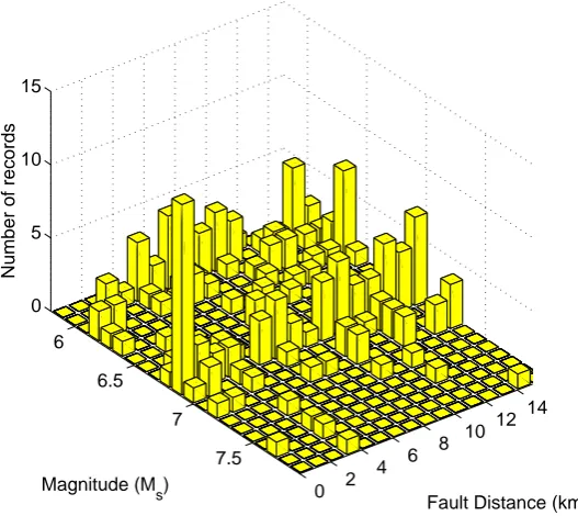
material are listed in Ambraseys and Douglas [3]. The distribution of the records

used with respect to geographical location and earthquake mechanism is given in

Table 1. Figure 1 shows the distribution of the data with magnitude and distance.

Although some authors have found evidence for differences in strong ground

mo-tions due to the tectonic environment [e.g. 28] the limited number of records

fulfill-ing our selection criteria meant that we could not investigate this effect. However,

all the records in our set came from active tectonic regions, except for two records

from the Nahanni earthquake (23/12/1985,Ms = 6.8) which is from a stable

con-tinental region.

As can be seen from Figure 1 the records are well distributed in magnitude and

well constrained and representative of the entire dataspace: 0 ≤ d ≤ 15 km and

5.8 ≤ Ms ≤ 7.8. The distribution with magnitude and distance of records from

thrust and strike-slip earthquakes is also reasonably uniform. There is a lack of

near-field recordings of earthquakes with normal mechanisms in the dataset used

and there are no records from normal earthquakes withMs >6.9because of fault

segmentation.

Site conditions at the stations are also given in Ambraseys and Douglas [3] using

the categorisation proposed by Boore et al. [9], i.e. L:Vs,30 < 180 ms−1 (very soft

soil), S: 180 ≤ Vs,30 < 360 ms−1 (soft soil), A: 360 ≤ Vs,30 < 750 ms−1 (stiff

soil), and R:Vs,30≥750 ms−1 (rock). Soil profiles for many of the Californian and

European stations are available, from which Vs,30 estimates were made directly.

For other sites, station conditions were assessed from the conversion of reported

site categories. Site conditions have been classified for 178 of the 186 records. The

distribution of the records used with respect to site classification is given in Table 1.

The difference between ground motions for sites on the hanging wall and foot wall

of faults [e.g. 2] is not considered here. This study uses distance to the surface

projection of the rupture,d, rather than the distance to the rupture therefore some

of the differences in estimated ground motions between hanging wall and foot wall

sites is implicitly modelled because hanging wall sites haved = 0 kmwhereas foot

wall sites haved >0 km, see for example Abrahamson and Somerville [2].

2.2 Correction procedure

Ideally all of the records used for this study should have been processed in a

uncor-rected format. Unfortunately some of the records (19) could only be obtained from

the original data owners in corrected format. Since these records came from large

earthquakes (the earthquakes hadMs = 6.5, 6.8, 7.0, 7.1and7.6), it was thought

better to incorporate them in this study. The short period range of interest for this

study of0.1to2.0 s, means that any differences in the correction procedure should

make little difference. The 19 records corrected in a different way are labelled in

Ambraseys and Douglas [3].

The uncorrected records were corrected using an elliptical filter [24] with pass band

0.2–25 Hz. For this study the values of these parameters used were: roll-off

fre-quency1.001 Hz, sampling interval0.02 s, ripple in pass-band0.005 and ripple in

stop-band0.015. This pass band was chosen because some of the records which we

could not obtain in uncorrected form were corrected with a similar pass band. Also

because of difference in quality between the different accelerograms used meant

that a narrower pass band should be used than when all the records are of a uniform

quality. The correction procedure though should not affect significantly the results

within the period of interest. An instrumental correction was applied if the

neces-sary characteristics were known for a particular record, most having the required

characteristics.

2.3 Model of ground motion

The ground motion model used has the form:

logy =b1+b2Ms+b3d+bASA+bSSS

of the rupture plane,SAtakes the value of 1if the site is classified as stiff soil (A)

and0otherwise, andSS takes the value of1if the site is classified as soft soil (S)

and0otherwise. For rock,SA=SS= 0.

The distance dependence was not defined in terms ofr = √d2_+h2 _{because if a}

depth term h is included it is almost indistinguishable from zero and hence was

dropped. Decay is assumed to be associated with anelastic effects due to large

strains, which is reasonable in the near field. Geometric decay close to the rupture

of large earthquakes is small because seismic waves are reaching the station from

many parts of the long rupture, unlike in the far field where the source can be

ap-proximated by a point and hence geometric decay is important. Also since both the

geometrical decay terms of the formlog(d)and the anelastic terms of the formdare

highly correlated within the short distance range used in the study, they cannot be

found simultaneously. A function of the form:logy =c1+c2Ms+c3log q

d2_+c2 4

was also tried and the results were almost identical to those for the adopted

func-tional form. Therefore the type of attenuation (geometric or anelastic) assumed is

unimportant for this set of records.

The largest horizontal component was used for deriving the following attenuation

relations for consistency with previous work. All peak ground acceleration and

spectral accelerations are in ms−2_{, all energy densities are in cm}2_s−1 _{and all}

max-imum absolute input energies are in cm2_s2_.

2.4 Regression method

A number of different regression methods exist for deriving attenuation relations,

of regression techniques used: one-stage [e.g. 4] and two-stage [e.g. 23]. In the

former the magnitude and distance coefficients are found simultaneously whereas

in the latter the distance coefficients are found first and then, in the second step the

magnitude coefficients are determined.

Within these categories there are also two further procedures, ordinary least squares

estimation and random-effects (or maximum-likelihood) models [11, 12]. The first

of these simply finds the coefficients which minimize the sum of squares of the

residuals considering the error in each record to be independent from the other

records. After the coefficients are determined the standard deviation is found for

the entire equation.

In the random-effects technique the error is assumed to consist of two parts: an

earthquake-to-earthquake component, which is the same for all records from the

same earthquake, and a record-to-record component, which expresses the

variabil-ity between each record not expressed by the earthquake-to-earthquake component.

The standard deviation of these two errors is found along with the coefficients. This

method is thought to take better account of the fact that each record from the same

earthquake is not strictly independent.

Most authors find that the regression technique used does not affect the results

obtained within the range of distance and magnitude that are of engineering interest

[4, 7]. However, some authors find that due to high correlation between a record’s

magnitude and distance, the one-stage method gives biased results [22, 21] and that

the two-stage technique eliminates this bias.

These two studies were based on Japanese datasets where the depths and distances

of the events are much larger than for this near-field study. In our case the

coeffi-cientrMs,d =−0.10. Therefore these results do not apply to this study.

Before deciding which regression method to use for this study, both one-stage and

two-stage ordinary least squares were used to peak ground acceleration and

spec-tral ordinates of the horizontal and vertical components. A comparison of the

re-sults shows almost identical distance dependence terms but quite large differences

in the magnitude terms. ForMs = 6.8the predicted PGA from the two methods are

similar, diverging for higher and lower magnitude. The two stage regression

pre-dicts higher accelerations for smaller magnitudes and lower accelerations for larger

magnitudes. This is also observed for vertical PGA, and for horizontal and vertical

spectral ordinates. These differences are found because the two-stage method gives

more weight to the less well recorded larger magnitude earthquakes (Ms > 7.0),

in particular the Kocaeli earthquake (17/8/1999,Ms = 7.8) which contributes two

records to the set, than does the one-stage method. The PGA of the two Kocaeli

records are much lower (ah = 3.5 ms−2 and ah = 2.2 ms−2) than would be

ex-pected from such a large magnitude earthquake. After removing the two Kocaeli

records from the set and repeating the regression analysis it was found that the

magnitude coefficient changed significantly (fromb2 = 0.151tob2 = 0.195) for the

two-stage method but less significantly for the one-stage method (fromb2 = 0.202

tob2 = 0.222) for horizontal PGA. It was felt that the two-stage method gave undue

weight to the two records from the Kocaeli earthquake, which may not be typical

of records from large magnitude earthquakes. Therefore, in what follows we shall

2.5 Effect of site geology

Site geology was included in this study following the methodology of Ambraseys

et al. [7]. The residuals:

i = log(yi)−b01−b2(Mi)−b3di

from the first stage of the regression are found. Then the regression is performed

on:

=b4SR+b5SA+b6SS

whereSR takes the value1if the site is classified as rock and0otherwise, andSA

and SS are similarly defined for stiff (A) and soft (S) soil sites. Then new

coeffi-cients are defined as follows:b1 = b01 +b4; bA = b5 −b4, and bS = b6 −b4, and

the errorσis recalculated with respect to the site-dependent prediction, using only

those records of known site conditions.

3 Results

Table 2 gives the coefficients and standard deviations of the equations for

horizon-tal peak ground acceleration (ah), vertical peak ground acceleration (av), vertical to

horizontal absolute peak ground acceleration ratio (q =av/ah), vertical to

horizon-tal simultaneous peak ground acceleration ratio (qsim), horizontal energy density

(Eh), vertical energy density (Ev) and vertical to horizontal energy density ratio

level is also given in Table 2. Only coefficients that are significant at the5% level

are retained; if a coefficient was not significant then the regression was repeated

with the coefficient which was not significant constrained to zero.

The vertical to horizontal simultaneous PGA ratio defined as,qsim =av(tmax)/ah,

where av(t) is the vertical ground acceleration time-history, ah is the horizontal

PGA andtmaxis the time at which this peak occurs. It gives the vertical acceleration

to be resisted by a structure at the time of the design horizontal acceleration.

The energy density,E, of an strong motion record is defined asE = 1₄SρRT

0 v(t)2dt,

whereT is the length of the record,v(t)is the ground velocity at timet, S is the

wave velocity of the material carrying the wave and ρ is the mass density in the

material [27]. In this article, equations are derived for the integral part of this

def-inition and hence do not include the effect of the wave velocity or mass density.

ThereforeEh =

RT

0 vh(t)2dt, wherevh(t)is the horizontal ground velocity at time

t, and Ev =

RT

0 vv(t)2dt, wherevh(t)is the horizontal ground velocity at time t.

To correctly use the equations derived here, the results must be multiplied by 1₄Sρ

to obtain the true energy density.

In this article, the estimated ground motions using the equations derived in this

study are compared with estimated ground motions using the equations from some

commonly cited studies, Boore et al. [9], Campbell and Bozorgnia [15], Ambraseys

et al. [7], Ambraseys and Simpson [5], Campbell [14], Chapman [16] and

Spu-dich et al. [28]. As in this study, the comparisons studies mainly use strong-motion

records from active tectonic regions, therefore the estimated ground motions from

this study and the comparison studies can be directly compared.

All of the comparison studies have included data from earthquakes with all three

which only includes data from strike-slip and normal faulting earthquakes in

ex-tensional regions. However, all the comparison studies, and also this study, include

limited numbers of strong-motion records from earthquakes with normal

mecha-nisms.

All of the comparison studies use a significant proportion of near-field records,

almost all of which are included within the set of records selected for this study.

However, these comparison studies also use many records from the intermediate

and far fields, which are of lower engineering significance. Therefore comparisons

in estimated ground motions using the equations from the comparison studies (from

a mix of near-, intermediate and far-field data) and those derived in this study (from

only near-field data) will show the effect of including data of lower engineering

significance in sets of records used to derive equations to estimate near-field ground

motions.

3.1 Horizontal PGA,y= log(ah)

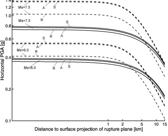
Figure 2 shows comparison between the horizontal PGA predicted by the new

equa-tion given in Table 2 and that predicted by four other widely used equaequa-tions.

Fig-ure 2 shows the following important featFig-ures.

The new equation predicts much lower accelerations than the equation of

Am-braseys et al. [7] especially for large magnitudes, for example for Ms = 7.5 and

d = 0 km the equation of Ambraseys et al. [7] predicts horizontal PGA for soft

soil of about1.4 g[14 ms−2] compared with the new equation which predicts

hor-izontal PGA for soft soil of about0.8 g[8 ms−2_{]. This over-estimation of PGA by}

ground motions in the records used. The new equation predicts similar horizontal

PGA to those predicted by the equations of Boore et al. [9] and Campbell [14]

re-flecting the large number of records from large magnitudes and short distances in

their sets. The new equation predicts slightly larger horizontal PGA than the

equa-tion of Spudich et al. [28] for extensional regimes, again confirming the finding of

Spudich et al. [28] that the strong ground motion in extensional regimes is smaller

than that in other tectonic regimes. Spudich et al. [28] use the geometric mean of

the two horizontal components rather than the larger horizontal component which

could be one factor reducing the predicted accelerations.

The new equation exhibits a lower dependence on magnitude than the equation of

Ambraseys et al. [7]. The coefficient of magnitude dependence in the equations

de-rived in this study is 0.202 as compared to 0.266 for the equations of Ambraseys

et al. [7]. The equation of Ambraseys et al. [7] was derived using mainly data

from small magnitude (Ms <6) earthquakes and so the point source assumption is

roughly valid and consequently the equation reflects global fault conditions. For the

data used to derive the new equation the point source assumption is not adequate

and so the equation reflects the local fault conditions leading to lower magnitude

dependence. The magnitude dependence however, is almost identical to that in the

equations of Boore et al. [9] and Spudich et al. [28] showing that these equations

can be used for ground motion estimation in the near-field. The magnitude

de-pendence of the new equation is larger than that of the equation of Campbell [14]

possibly due to the form of the equation adopted by Campbell [14] which allows for

distance saturation or because of the distance measure used by Campbell [14]

(seis-mogenic distance) differs from that used here (distance to the surface projection of

the rupture plane).

et al. [9] and Spudich et al. [28] and is similar to that of Ambraseys et al. [7] and

Campbell [14] showing that the attenuation mechanism that is dominant in the

near-field cannot be determined. This can be seen in Figure 2 because the new curves

are almost parallel to the curves derived in the other studies.

The new equation predicts near-field horizontal PGA which is almost independent

of site conditions, unlike the equations of Boore et al. [9], Ambraseys et al. [7] and

Spudich et al. [28] which show significant dependence of horizontal PGA with site

conditions. This can be seen in Figure 2 because the predicted PGAs for all three

local site conditions are almost identical (because the site coefficients are small)

whereas the predicted PGAs using the equations of Boore et al. [9], Ambraseys

et al. [7] and Spudich et al. [28] for different local site conditions vary significantly

(because the site coefficients are much larger). The site dependence is also lower

than that predicted by the equation of Campbell [14] which allows for site

amplifi-cations which are dependent on magnitude and distance. The negligible dependence

of near-field horizontal PGA on site conditions shows, as pointed out by Faccioli

and Rese´ndiz [19], that close to the source, site conditions are less important in

determining ground motions than source and path. Also it may indicate non-linear

soil behaviour at large strains which occur in the near field of large earthquakes

leading to lower soil amplification than for weak ground motions.

The associated standard deviation of the new equation (σ = 0.214) is slightly

smaller than that of the equation of Ambraseys et al. [7] (σ = 0.25) but similar

to that of Boore et al. [9] (σ = 0.205), Spudich et al. [28] (σ = 0.204) and

Camp-bell [14] (0.169–0.239 dependent on horizontal PGA). This shows that near-field

horizontal PGA is not less variable than intermediate-field and far-field horizontal

3.2 Vertical PGA,y = log(av)

A comparison of the new equations for horizontal and vertical PGA shows that the

decay with distance of vertical PGA is faster than that of horizontal PGA. This is

probably because vertical ground motions are generally of higher frequency than

horizontal ground motions (high frequency waves attenuate more rapidly than low

frequency waves). Further, the standard deviation of an observation for the new

equation for vertical PGA is much larger than that of the new equation for

hori-zontal PGA. Currently, the reason that the estimation of vertical PGA is associated

with larger uncertainty than the estimation of horizontal PGA is unknown.

Figure 3 shows comparisons between the peak ground acceleration predicted by

the new equation and that predicted by two other widely-used equations. Figure 3

shows the following important features.

The new equation predicts slightly larger vertical PGA than the equation of

Am-braseys and Simpson [5] and lower vertical PGA, especially for earthquakes with

magnitudes aboutMs = 6, than the equation of Campbell [14].

The dependence of vertical PGA on site conditions is similar to that predicted by the

equations of Ambraseys and Simpson [5] and Campbell [14] showing that nonlinear

soil behaviour at large strains is apparently not as common for vertical ground

motions as is for horizontal motions.

As for horizontal PGA the associated standard deviation (σ = 0.270) is similar to

that from the equation of Ambraseys and Simpson [5] (σ = 0.25) and Campbell

3.3 Vertical to horizontal absolute PGA ratio,y = logq= log(av/ah)

The ratioq, of the vertical,av, to the maximum horizontal,ah, ground acceleration

can be calculated either by combining the two equations which individually

pre-dict peak vertical and horizontal accelerations [1], or by performing a regression

directly on the ratios of maximum accelerations [4]. Note that whereas Ambraseys

and Simpson [5, 6] regress directly on the ratio,av/ah, in this study the regression

was made on the logarithm of the ratio. This is because the derived equation has a

physical interpretation, i.e. exponential dependence on magnitude and decay due to

anelastic effects. Also, directly using the ratios of maximum acceleration assumes

that the uncertainty associated with this ratio is the same for all levels of ground

motion [17, pp. 237–238]. This assumption must be false because otherwise

us-ing the standard deviation associated with the equation, to derive predicted ratios

for percentiles less than 50%, would lead to the prediction of negative PGA (by

definition a positive quantity). Also working directly on the untransformed ratio

violates the requirement of the standard least-squares method that the residuals be

homoscedastic, i.e. that the residuals are similarly distributed with respect to the

predicted value and the independent parameters.

No site coefficients were derived because they do not have a physical meaning,

unlike those for horizontal and vertical components separately. This is because for

horizontal and vertical ground motions separately the site coefficients are directly

connected to the amplifications due to the local site conditions in the direction,

i.e. horizontal or vertical, of interest whereas for the ratio of vertical to horizontal

motions any site coefficients derived would be due to a combination of

amplifica-tions in both the horizontal and vertical direcamplifica-tions. Since Ambraseys and Simpson

depend-ing on earthquake mechanism, the effect of earthquake mechanism is investigated

here. Vertical to horizontal ground motion ratios are more stable than horizontal or

vertical ground motions separately, therefore the effect of earthquake mechanism

on vertical to horizontal ratios could be considered whereas the limited number of

records precludes an investigation of the effect of earthquake mechanism on

hori-zontal and vertical ground motions separately.

Figure 4 shows comparison between the ratio of vertical PGA to horizontal PGA

predicted by the equations given in Table 2 and that predicted by equations from

two other widely used studies. Figure 4 shows the following important features.

The equations given in Table 2 predict much smaller ratios of vertical to

horizon-tal PGA than do the equations of Ambraseys and Simpson [5] and Campbell and

Bozorgnia [15]. The equations of Ambraseys and Simpson [5] predict larger ratios

because they use: a) a non-physical model which assumes error is additive rather

than multiplicative; b) only records with vertical PGA larger than0.1 gthereby

bi-asing the ratios upwards; c) the largest vertical to horizontal PGA ratio (i.e.

small-est horizontal component) rather than smallsmall-est vertical to horizontal PGA ratio (i.e.

largest horizontal component); and d) a small set of records. One reason Campbell

and Bozorgnia [15] predict larger ratios is that they use the geometric mean of the

two horizontal PGAs rather than the larger horizontal PGA. The larger horizontal

PGA is usually found to be about13%larger than the geometric mean of the two

horizontal PGAs [e.g. 13], therefore when the larger horizontal PGA is used lower

vertical to horizontal PGA ratios are found compared to when the geometric mean

of the two horizontal PGAs are used.

The equations given in Table 2, the equations of Ambraseys and Simpson [5], and

to horizontal PGA ratios for strike-slip faulting than thrust faulting.

The equations given in Table 2 show that the commonly used ratios between

ver-tical and horizontal PGA,q, of 1₂ to 2₃ are reasonable. However, sinceq represents

the ratio of two functions whose maxima occur at different times, its value is a

con-servative estimate of the combined loading that could occur during an earthquake.

3.4 Horizontal spectral acceleration,y= log SAh

The coefficients of the horizontal and vertical spectral acceleration equations for

5% damping at 46 periods between 0.1 and 2 s and different site conditions are

given in Ambraseys and Douglas [3]. The coefficients of the equations for a subset

of periods are given in Tables 3 and 4.

Comparing the predicted horizontal spectral accelerations using the new equations

with those predicted by four other widely used sets of equations shows a number

of important features (Figures 5 to 8).

Predicted horizontal spectral accelerations using the new equations are much lower

than those predicted by the equations of Ambraseys et al. [7] for large magnitudes

(Ms > 6.5) especially for very short distances, for example at horizontal natural

periodT = 0.5 sthe equations of Ambraseys et al. [7] predict a spectral

accelera-tion on soft soil of about2.3 g[23 ms−2_{]whereas using the new equations gives an}

estimate of about1.4 g[14 ms−2_{]. This is similar to the earlier finding for}

horizon-tal PGA, i.e. the equations of Ambraseys et al. [7] predicted much larger horizonhorizon-tal

PGAs for large magnitude earthquakes than the equations derived in this study. The

reason for such large differences for large magnitudes is that the set of records used

which control the equation. The magnitude dependence for the short period range

(T <1 s) of the near-field equations derived in this study is much less than that in

the equations of Ambraseys et al. [7] so the predicted accelerations for large

mag-nitude earthquakes are less. The equations of Boore et al. [9], Campbell [14] and

Spudich et al. [28] however, predict horizontal response spectra similar to those

given by the new equations because their sets have a large proportion of near-field

large-magnitude data and they include terms to account for magnitude saturation

which means the predicted spectral accelerations for large magnitudes do not

be-come unrealistically large.

As for horizontal PGA the dependence of spectral acceleration on site conditions

is much less in the near-field equations derived in this study than that found in the

equations of Ambraseys et al. [7], Boore et al. [9] and Spudich et al. [28] especially

in the very short period range (T < 0.2 s). This is probably due to nonlinear soil

behaviour due to large strains which would reduce the short period ground motion

more than the longer period ground motion, such behaviour is modelled in the

equations of Campbell [14].

As for the equation for horizontal PGA the near-field equations derived in this study

are associated with similar standard deviations as the equations of Ambraseys et al.

[7], Boore et al. [9], Campbell [14] and Spudich et al. [28].

3.5 Vertical spectral acceleration,y= log SAv

Vertical spectral acceleration for periods less than about1 sshow faster decay with

distance than horizontal spectral accelerations. Unlike the PGA this faster decay

than the horizonal motions because spectral acceleration is a narrow-band measure.

As for PGA the standard deviations associated with the near-field equations for

vertical spectral acceleration derived here are much higher than those for horizontal

spectral acceleration, especially for short periods. For example for T = 0.1 s the

standard deviation for horizontal spectral acceleration is0.240whereas for vertical

spectral acceleration it is0.308.

Soil coefficients for both soft (S) and stiff (A) soil show de-amplification, with

respect to rock, at long periods (T > 1 s).

Comparing the predicted vertical spectral accelerations using the new equations

with those predicted by two other widely used sets of equations shows a number of

important features (Figures 9 and 10).

Predicted vertical spectral accelerations using the new equations are similar to those

predicted by the equations of Ambraseys and Simpson [5] and Campbell [14]

ex-cept in the short period where the equations of Campbell [14] predict higher values,

for example forMs = 7.5andd= 0 kmthe predicted spectral acceleration on rock

using the new equations is about0.8 g[8 ms−2_{]whereas on soft rock using the}

equa-tions of Campbell [14] it is about1.4 g[14 ms−2_{]. This difference could be due to}

the different definition of distance used by Campbell [14] compared to that used

here.

The dependence of site conditions on vertical spectral accelerations in the

near-field equations is similar to that found by Ambraseys and Simpson [5] and is much

less than that found for horizontal spectral accelerations. The dependence on site

conditions is less than that found by Campbell [14] which could be due to the

different site categories used or because the vertical spectral acceleration equation

as a base.

Comparing predicted horizontal response spectra (Figures 5 to 8) with predicted

vertical response spectra (Figures 9 and 10) shows the expected higher frequency

of vertical ground motions.

3.6 Horizontal and vertical maximum absolute input energy,y= logIh andy =

logIv

The coefficients of the horizontal and vertical maximum absolute input energy

equations for5%damping at 46 periods between0.1and2 sand different site

con-ditions are given in Ambraseys and Douglas [3]. The coefficients of the equations

for a subset of periods are given in Tables 5 and 6.

The maximum absolute input energy,I, is defined asI = maxtR0t[utt(t)+a(t)]v(t) dt,

whereuttis the response acceleration of the SDOF system,a(t)is the ground

accel-eration andv(t)is the ground velocity [16]. In the following two sections maximum

absolute input energy will simply be referred to as energy.

The new equations show that there is a strong dependence of horizontal maximum

absolute input energy on magnitude as is expected because magnitude is roughly

related to energy. The coefficients also display a faster decay with distance than

spectral acceleration and also a stronger dependence on site conditions. The

stan-dard deviations of the equations for horizontal energy are also much higher than

those for horizontal spectral acceleration, for example for T = 0.1 s the

associ-ated standard deviation for horizontal spectral acceleration is 0.240 whereas for

Comparing the predicted energy using the new equations with those predicted by

the only other set of attenuation relations [16] for horizontal energy available in the

literature (Figure 11) shows the following important features.

Predicted horizontal energies using the new equations are similar to those predicted

by the equations of Chapman [16] because many of the records used by Chapman

[16] are from large earthquakes and also because the equations allow magnitude

saturation. The predicted energies are thus not unrealistically high.

As for horizontal PGA and spectral acceleration there is evidence for nonlinear

soil behaviour in the near-field because the dependence of horizontal energy on

local site conditions is less than the dependence found by Chapman [16] who uses

intermediate-field and far-field records as well as near-field records.

The standard deviations of the near-field equations derived in this study and those

of the equations of Chapman [16] are similar.

As for horizontal energy there is a strong dependence of vertical energy on

mag-nitude, a faster decay with distance than for vertical spectral acceleration, greater

dependence on local site conditions and also much larger associated standard

devi-ations than the equdevi-ations for vertical spectral acceleration.

As for vertical spectral acceleration and horizontal spectral acceleration there is

much lower dependence of vertical energy on local site conditions than for

hori-zontal energy.

No attenuation relations for the prediction of vertical elastic maximum absolute

input energy such as have been derived here (Figure 12) appear to have been

3.7 Vertical to horizontal spectral ratio (absolute),y= logqs = log SAv/SAh

There are two methods for finding the predicted vertical to horizontal spectral

ra-tios a) divide the predicted vertical spectral accelerations by the predicted

horizon-tal accelerations or b) regress directly on the spectral ratio to find new attenuation

equations for the ratio. The first technique was used by Niazi and Bozorgnia [25],

Bozorgnia et al. [10] and Campbell and Bozorgnia [15]. Its main advantage is

sim-plicity. The second technique was used by Feng et al. [20] and Ambraseys and

Simpson [5].

Equations to predict the vertical to horizontal spectral ratio, qs, were derived

as-suming magnitude and distance dependence. For some periods, the magnitude

co-efficient is significant, for some the distance coco-efficient is significant but for most

neither are significant. Therefore it was decided to simply provide the mean of the

logarithms and the standard error. Note that even though the magnitude and

dis-tance coefficients of the horizontal and vertical spectral acceleration equations are

significant at the5%level the coefficients for prediction of the ratio are not.

There-fore workers who find distance and magnitude dependence of the spectral ratios

[e.g. 25, 10, 15] from regressing on the horizontal and vertical spectral ordinates

separately may find that this dependence is not significant if the regression is done

directly on the ratio.

The coefficients of the vertical to horizontal spectral ratio equations for5%

damp-ing at 46 periods between 0.1 and 2 s and different site conditions are given in

Ambraseys and Douglas [3]. No site coefficients were derived. The coefficients of

the equations for a subset of periods are given in Table 7.

equa-tions with those predicted by two other widely used sets of equaequa-tions (Figures 13 and 14)

show the following important features.

Predicted vertical to horizontal spectral ratios using the new equations are much

lower than those predicted using the equations of Ambraseys and Simpson [5] for

the same reasons that the predicted vertical to horizontal PGA ratios were lower.

However, predicted vertical to horizontal spectral ratios using the new equations

and those predicted using the equations of [15] are almost identical except for short

periods (T < 0.4 s) where the equations of Campbell and Bozorgnia [15] predict

higher ratios; this is similar to the vertical to horizontal PGA ratios.

Predicted vertical to horizontal spectral ratios using the new equations for all source

mechanisms, except for normal faulting, are almost identical, as was found by

Campbell and Bozorgnia [15]. The apparent differences for different source

mech-anisms found by Ambraseys and Simpson [5] are probably due to: a) the

non-physical model used by Ambraseys and Simpson [5] which assumes error is

addi-tive rather than multiplicaaddi-tive and b) the small set of records. The differences in

the vertical to horizontal spectral ratios found for normal faulting earthquakes may

not be genuine because only a small number of records (15) from normal faulting

earthquakes were used.

3.8 Vertical to horizontal spectral ratio (simultaneous),y = logqi = log(utt,v(tmax)/SAh)

A major draw-back of the absolute acceleration ratioqorqsfor practical purposes is

that in an earthquake the maximum ground or response accelerations in the vertical

and horizontal direction occur at different times.

ratio were found. This ratio is defined as: qi = utt,v(tmax)/SAh; where utt,v(t) is

the vertical response acceleration andtmaxis the time as which the maximum

hor-izontal response acceleration occurs. This ratio gives the size of the vertical

accel-erations which need to be withstood at the time of the design maximum horizontal

acceleration.

The natural period of a structure in the vertical direction is usually different than

that in the horizontal direction therefore these ratios,Qi, were found for all

combi-nations of vertical and horizontal natural period, i.e.46×46 = 2116.

As for the absolute ratio, for some periods the magnitude coefficient is significant,

for some the distance coefficient is significant but for most neither are significant.

Therefore it was decided to simply provide the mean of the logarithms and the

standard error.

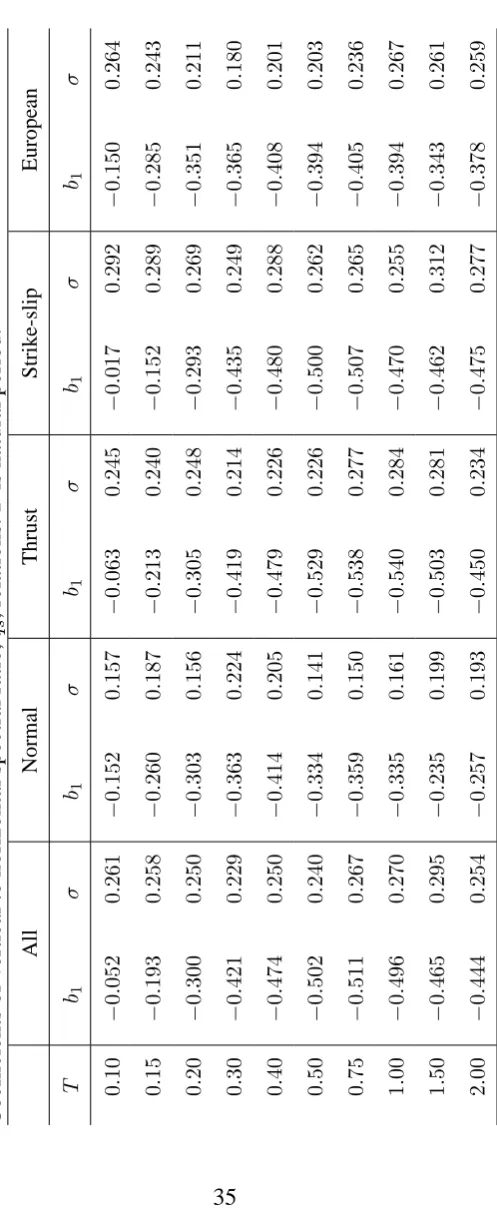
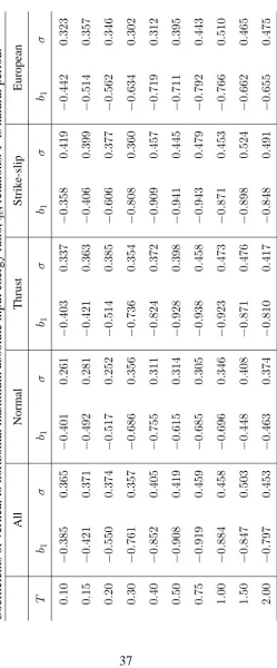
The means and standard deviations for all earthquakes, normal, thrust and

strike-slip and European earthquakes separately for 5% damping at 46 periods between

0.1and2 sand different site conditions are given in Ambraseys and Douglas [3].

The coefficients of the equations for a subset of periods are given in Table 8.

The predicted qi for all the earthquakes and for each of the separate mechanism

(normal, thrust and strike-slip) shows that the ratios are almost the same for each

type of faulting except for normal faulting (Figure 15). The results for normal

mechanism earthquakes are based on only15records; it is difficult to base

conclu-sions on such a small number of records so more records are required from normal

earthquakes to check this finding. As Figure 15 shows the simultaneous ratios,qi,

are much less than the absolute ratios,qs, especially for short periods. Also it can

Figure 16 shows the predicted vertical to horizontal simultaneous spectral ratio,Qi,

for all combinations ofTh andTv. Figure 17 shows the standard deviations (this is

the standard deviations of the logarithms) of the regression.

For short vertical and long horizontal periods the simultaneous ratio,Qi, can reach

about0.5but for most periods the ratio is less than about0.2(Figure 16). The

stan-dard error is much higher than for the absolute ratio and it is roughly independent

of period and equal to about0.6(Figure 17). Why there are much higher standard

errors at certain, seemingly random, combinations of periods is not known.

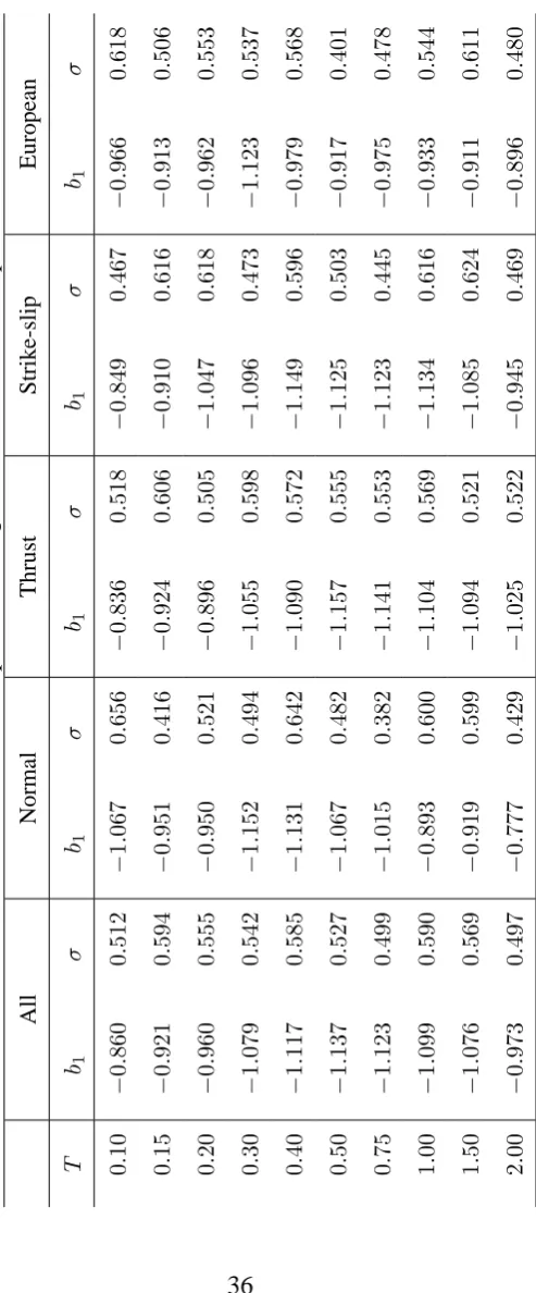
3.9 Vertical to horizontal maximum absolute input energy ratio, y = logqe =

logIv/Ih

The means and standard deviations oflogqefor all earthquakes, normal, thrust and

strike-slip and European earthquakes separately for5% damping at 46 periods

be-tween0.1and2 sand different site conditions are given in Ambraseys and Douglas

[3]. The coefficients of the equations for a subset of periods are given in Table 9.

Figure 18 shows the predicted ratio, qe, for all earthquakes and considering the

three source mechanisms separately. As for the response spectral equations only

predicted ratios for normal mechanism earthquakes are different than those for

other types of faulting, although this may be due to a small number of records from

normal earthquakes. Figure 18 shows that even for short periods vertical ground

4 Conclusions

The ratio of the maximum peak ground acceleration to maximum horizontal in an

earthquake, which individually occur at different instants, may exceed one, but their

ratioqfalls off with distance. Due to lack of data for strike-slip and normal events

the magnitude and distance dependence of the ratio,q, cannot be found but the mean

ratios are0.73and0.61respectively, hence they are close to the commonly accepted

ratio of 2₃. The complete near-field dataset and the thrust subset show significant

distance dependence, the ratios decrease with distance, and the predicted ratios

also are close to 2₃. Note, that the maximum values of the vertical and horizontal

peak acceleration in this ratio occur at different times in an earthquake.

The spectral response of the vertical acceleration and the attenuation of its spectral

ordinates with magnitude and distance differ in amplitude and shape from those of

the horizontal.

The ratioqsof the maximum vertical spectral response to the horizontal may exceed

one at very short periods (< 0.15 s), but falls off rapidly with period reaching a

value of about0.5for long periods. Note that maximum spectral values of this ratio

occur at different times but for the same response period in both horizontal and

vertical direction (Th =Tv).

The ratio of the vertical spectral response that occurs at the time of the maximum

horizontal responseqi does not exceed0.2and is insensitive to magnitude and

dis-tance. Note that in this case the response period in the horizontal and vertical

direc-tions are equal.

remains smaller than0.3. The exception is for the rather unrealistic combination of

very short vertical periods (0.1 s) with very long horizontal (> 1.0 s) for whichq

may reach0.6.

For elastic structures the energy input from the vertical component is a small

frac-tion of the energy input due to the horizontal.

5 Acknowledgements

We would like to thank all the colleagues who gave us their views regarding the

effect of vertical motion on design. Also, we would like to thank Drs. K. Simpson,

M. Srbulov, M. Free and S.K. Sarma and P. Smit for their help in this research

which was supported by EPSRC. In addition, critical reviews by two anonymous

reviewers were helpful and lead to significant improvements to the article.

References

[1] Abrahamson, N. A., Litehiser, J. J., Jun 1989. Attenuation of vertical peak

acceleration. Bulletin of the Seismological Society of America 79 (3), 549–

580.

[2] Abrahamson, N. A., Somerville, P. G., Feb 1996. Effects of the hanging wall

and footwall on ground motions recorded during the Northridge earthquake.

Bulletin of the Seismological Society of America 86 (1B), S93–S99.

[3] Ambraseys, N., Douglas, J., Aug 2000. Reappraisal of the effect of vertical

ground motions on response. ESEE Report 00-4, Department of Civil and

Environmental Engineering, Imperial College, London.

acceler-ations in Europe. Earthquake Engineering and Structural Dynamics 20 (12),

1179–1202.

[5] Ambraseys, N. N., Simpson, K. A., 1996. Prediction of vertical response

spec-tra in Europe. Earthquake Engineering and Structural Dynamics 25 (4), 401–

412.

[6] Ambraseys, N. N., Simpson, K. A., 1997. The effect of vertical acceleration

on horizontal response. ESEE report, Department of Civil and Environmental

Engineering, Imperial College, London.

[7] Ambraseys, N. N., Simpson, K. A., Bommer, J. J., 1996. Prediction of

hor-izontal response spectra in Europe. Earthquake Engineering and Structural

Dynamics 25 (4), 371–400.

[8] Benavent-Climent, A., Pujade, L. G., L`opez-Almansa, F., 2002. Design

en-ergy input spectra for moderate-seismicity regions. Earthquake Engineering

and Structural Dynamics 31, 1151–1172.

[9] Boore, D. M., Joyner, W. B., Fumal, T. E., 1993. Estimation of response

spec-tra and peak accelerations from western North American earthquakes: An

in-terim report. Open-File Report 93-509, U.S. Geological Survey.

[10] Bozorgnia, Y., Campbell, K. W., Niazi, M., 2000. Observed spectral

character-istics of vertical ground motion recorded during worldwide earthquakes from

1957 to 1995. In: Proceedings of Twelfth World Conference on Earthquake

Engineering. Paper No. 2671.

[11] Brillinger, D. R., Preisler, H. K., 1984. An exploratory analysis of the

Joyner-Boore attenuation data. Bulletin of the Seismological Society of America

74 (4), 1441–1450.

[12] Brillinger, D. R., Preisler, H. K., 1985. Further analysis of the Joyner-Boore

attenuation data. Bulletin of the Seismological Society of America 75 (2),

[13] Campbell, K. W., Dec 1981. Near-source attenuation of peak horizontal

accel-eration. Bulletin of the Seismological Society of America 71 (6), 2039–2070.

[14] Campbell, K. W., Jan/Feb 1997. Empirical near-source attenuation

relation-ships for horizontal and vertical components of peak ground acceleration,

peak ground velocity, and pseudo-absolute acceleration response spectra.

Seismological Research Letters 68 (1), 154–179.

[15] Campbell, K. W., Bozorgnia, Y., Nov 2000. New empirical models for

predict-ing near-source horizontal, vertical, andV /H response spectra: Implications

for design. In: Proceedings of the Sixth International Conference on Seismic

Zonation.

[16] Chapman, M. C., Nov 1999. On the use of elastic input energy for seismic

hazard analysis. Earthquake Spectra 15 (4), 607–635.

[17] Draper, N. R., Smith, H., 1981. Applied Regression Analysis, 2nd Edition.

John Wiley & Sons.

[18] Ekstr¨om, G., Dziewonski, A. M., Mar 1988. Evidence of bias in estimations

of earthquake size. Nature 332, 319–323.

[19] Faccioli, E., Rese´ndiz, D., 1976. Soil dynamics: Behavior including

liquefac-tion. In: Lomnitz, C., Rosenblueth, E. (Eds.), Seismic Risk and Engineering

Decisions. Elsevier Scientific Publishing Company, Ch. 4, pp. 71–139.

[20] Feng, D., Theofanopoulos, N., Watabe, M., 1988. Consideration on the design

velocity response spectra along the principal axes. In: Proceedings of Ninth

World Conference on Earthquake Engineering. Vol. II. pp. 855–860.

[21] Fukushima, Y., Tanaka, T., 1990. A new attenuation relation for peak

horizon-tal acceleration of strong earthquake ground motion in Japan. Bulletin of the

Seismological Society of America 80 (4), 757–783.

[22] Fukushima, Y., Tanaka, T., Kataoka, S., 1988. A new attenuation relationship

Proceedings of Ninth World Conference on Earthquake Engineering. Vol. II.

pp. 343–348.

[23] Joyner, W. B., Boore, D. M., Dec 1981. Peak horizontal acceleration and

ve-locity from strong-motion records including records from the 1979 Imperial

Valley, California, earthquake. Bulletin of the Seismological Society of

Amer-ica 71 (6), 2011–2038.

[24] Menu, J. M. H., 1986. Engineering study of near-field earthquake

strong-motions. Ph.D. thesis, University of London.

[25] Niazi, M., Bozorgnia, Y., 1992. Behaviour of near-source vertical and

hori-zontal response spectra at SMART-1 array, Taiwan. Earthquake Engineering

and Structural Dynamics 21, 37–50.

[26] S¸afak, E., 2000. Characterization of seismic hazard and structural response by

energy flux. Soil Dynamics and Earthquake Engineering 20, 39–43.

[27] Sarma, S. K., 1971. Energy flux of strong earthquakes. Tectonophysics 11,

159–173.

[28] Spudich, P., Joyner, W. B., Lindh, A. G., Boore, D. M., Margaris, B. M.,

Fletcher, J. B., Oct 1999. SEA99: A revised ground motion prediction relation

for use in extensional tectonic regimes. Bulletin of the Seismological Society

Table 1

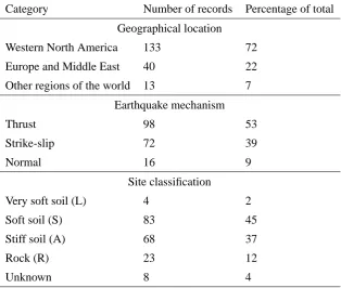
Summary of distribution of data in the set of records used with respect to geographical location, faulting mechanism and site classification. Note, percentages do not add up to 100% because of rounding.

Category Number of records Percentage of total

Geographical location

Western North America 133 72

Europe and Middle East 40 22

Other regions of the world 13 7

Earthquake mechanism

Thrust 98 53

Strike-slip 72 39

Normal 16 9

Site classification

Very soft soil (L) 4 2

Soft soil (S) 83 45

Stiff soil (A) 68 37

Rock (R) 23 12

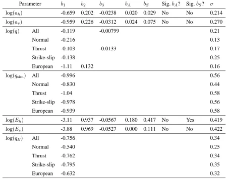
Table 2

Coefficients of equations for estimation of horizontal peak ground acceleration (ah), verti-cal peak ground acceleration (av), vertical to horizontal absolute peak ground acceleration ratio (q), vertical to horizontal simultaneous peak ground acceleration ratio (qsim),

hori-zontal energy density (Eh), vertical energy density (Ev) and vertical to horizontal energy density ratio (qE). Column labelled ‘Sig.bA?’ states whether thebAcoefficient is signifi-cant at the5%significance level, ‘Sig.bS?’ states whether thebS coefficient is significant at the5%significance level andσis the standard deviation of the equation.

Parameter b1 b2 b3 bA bS Sig.bA? Sig.bS? σ

log(ah) -0.659 0.202 -0.0238 0.020 0.029 No No 0.214

log(av) -0.959 0.226 -0.0312 0.024 0.075 No No 0.270

log(q) All -0.119 -0.00799 0.21

Normal -0.216 0.13

Thrust -0.103 -0.0133 0.17

Strike-slip -0.138 0.25

European -1.11 0.132 0.16

log(qsim) All -0.996 0.56

Normal -0.830 0.44

Thrust -1.04 0.58

Strike-slip -0.978 0.56

European -0.939 0.58

log(Eh) -3.11 0.937 -0.0567 0.180 0.417 No Yes 0.419

log(Ev) -3.88 0.969 -0.0527 0.000 0.111 No No 0.422

log(qE) All -0.756 0.34

Normal -0.540 0.25

Thrust -0.762 0.34

Strike-slip -0.795 0.35

Table 3

Coefficients of horizontal spectral acceleration relations. T is natural period. Soil coeffi-cients labelled with (*) are significant at the5%level.

T b1 b2 b3 bA bS σ

0.10 0.028 0.143 −0.0238 −0.042 −0.014 0.240

0.15 0.110 0.135 −0.0189 0.001 0.001 0.251

0.20 −0.182 0.175 −0.0164 0.006 0.049 0.251

0.30 −0.554 0.231 −0.0251 0.057 0.117(*) 0.251

0.40 −0.714 0.246 −0.0263 0.086 0.119(*) 0.256

0.50 −0.992 0.275 −0.0252 0.110 0.178(*) 0.253

0.75 −1.182 0.291 −0.0352 0.113 0.220(*) 0.264

1.00 −1.726 0.347 −0.0307 0.153(*) 0.220(*) 0.272

1.50 −2.904 0.492 −0.0298 0.128 0.225(*) 0.276

2.00 −3.380 0.543 −0.0326 0.098 0.215(*) 0.262

Table 4

Coefficients of vertical spectral acceleration relations.T is natural period. Soil coefficients labelled with (*) are significant at the5%level.

T b1 b2 b3 bA bS σ

0.10 −0.513 0.209 −0.0287 0.025 0.113 0.308

0.15 −0.706 0.226 −0.0268 0.070 0.118 0.287

0.20 −0.858 0.241 −0.0275 0.056 0.066 0.282

0.30 −1.106 0.261 −0.0265 0.050 0.012 0.256

0.40 −1.547 0.309 −0.0292 0.108(*) 0.043 0.255

0.50 −1.524 0.302 −0.0325 0.081 0.015 0.243

0.75 −1.855 0.337 −0.0364 0.057 −0.006 0.258

1.00 −2.294 0.384 −0.0335 0.028 0.021 0.259

1.50 −2.981 0.466 −0.0292 −0.072 −0.055 0.285

Table 5

Coefficients of horizontal maximum absolute input energy relations.T is natural period. Soil coefficients labelled with (*) are significant at the5%level.

T b1 b2 b3 bA bS σ

0.10 −0.874 0.613 −0.0593 0.041 0.169 0.397

0.15 −0.181 0.529 −0.0492 0.082 0.133 0.413

0.20 −0.156 0.539 −0.0426 0.052 0.171 0.412

0.30 −0.381 0.600 −0.0504 0.120 0.271(*) 0.435

0.40 −0.429 0.617 −0.0512 0.195 0.257(*) 0.458

0.50 −0.743 0.662 −0.0471 0.215 0.344(*) 0.478

0.75 −0.519 0.639 −0.0640 0.243 0.460(*) 0.499

1.00 −1.291 0.740 −0.0560 0.296(*) 0.440(*) 0.523

1.50 −3.198 1.005 −0.0509 0.262 0.487(*) 0.502

2.00 −3.700 1.074 −0.0593 0.206 0.464(*) 0.487

Table 6

Coefficients of vertical maximum absolute input energy relations.T is natural period. Soil coefficients labelled with (*) are significant at the5%level.

T b1 b2 b3 bA bS σ

0.10 −0.986 0.572 −0.0585 −0.009 0.177 0.477

0.15 −0.928 0.576 −0.0522 0.093 0.194 0.505

0.20 −1.096 0.606 −0.0508 0.112 0.154 0.499

0.30 −1.327 0.644 −0.0497 0.088 0.064 0.457

0.40 −1.673 0.689 −0.0528 0.184 0.122 0.465

0.50 −1.532 0.675 −0.0571 0.177 0.098 0.457

0.75 −1.589 0.699 −0.0652 0.144 0.067 0.476

1.00 −2.044 0.762 −0.0600 0.090 0.105 0.488

1.50 −3.177 0.932 −0.0516 −0.079 −0.010 0.521

Figure captions

(1) Distribution of all records in new near-field dataset with respect to magnitude

and distance.

(2) Comparison of predicted horizontal PGA (new equation, solid lines) and that

predicted using the equations of Ambraseys et al. [7], Boore et al. [9],

Camp-bell [14] and Spudich et al. [28] (dashed lines) forMs= 6,7.5(corresponding

toMw = 6.1,7.5using equation (2) of Ekstr¨om and Dziewonski [18]) for

dif-ferent site categories. The equation of Campbell [14] is plotted for strike-slip

faulting assuming a vertical rupture plane and depth to top of seismogenic

zone of3 km. Note the new equation is converted to gwhen plotted.

(a) Comparison with Ambraseys et al. (1996) (dashed lines). S is for180 ≤

Vs,30 <360 ms−1 (soft soil) sites, A is for360 ≤Vs,30 < 750 ms−1 (stiff

soil) sites and R is forVs,30 ≥750 ms−1 (rock) sites.

(b) Comparison with Boore et al. (1993) (larger component) (dashed lines).

A is forVs,30≥750 ms−1sites, B is for360≤Vs,30<750 ms−1sites and

C is for180 ≤Vs,30 <360 ms−1 sites.

(c) Comparison with Campbell (1997) (dashed lines). FS is for alluvial or

firm soil sites, SR is for soft rock sites and HR is for hard rock sites.

(d) Comparison with Spudich et al. (1999) (dashed lines).

(3) Comparison of predicted vertical PGA (new equation, solid lines) and that

predicted using the equations of Ambraseys and Simpson [5] and Campbell

[14] (dashed lines) for Ms = 6, 7.5 (corresponding toMw = 6.1, 7.5 using

equation (2) of Ekstr¨om and Dziewonski [18]) for different site categories.

The equation of Campbell [14] is plotted for strike-slip faulting assuming a

vertical rupture plane and depth to top of seismogenic zone of3 km. Note the

(a) Comparison with Ambraseys & Simpson (1996) (dashed lines). S is for

180≤Vs,30 <360 ms−1(soft soil) sites, A is for360≤Vs,30<750 ms−1

(stiff soil) sites and R is forVs,30 ≥750 ms−1 (rock) sites

(b) Comparison with Campbell (1997) (dashed lines). FS is for alluvial or

firm soil sites, SR is for soft rock sites and HR is for hard rock sites.

(4) Comparison of predicted ratios of vertical PGA to horizontal PGA (Table 2,

solid lines) and those predicted using the equations of Ambraseys and

Simp-son [5] and Campbell and Bozorgnia [15] (dashed lines) forMs = 6,7.5

(cor-responding toMw = 6.1, 7.5using equation (2) of Ekstr¨om and Dziewonski

[18]) for different source mechanisms. The equation of Campbell and

Bo-zorgnia [15], for the ratio of uncorrected vertical PGA to horizontal PGA, is

plotted for Holocene soil assuming a vertical rupture plane and depth to top

of seismogenic zone of3 km.

(a) Comparison with Ambraseys & Simpson (1996) (dashed lines).

(b) Comparison with Campbell & Bozorgnia (2000) (dashed lines).

(5) Comparison of predicted horizontal response spectra using the new equations

(solid lines) and those predicted using the equations of Ambraseys et al. [7]

(dashed lines) forMs = 6andd= 15 kmand forMs= 7.5andd= 5 kmfor

different site categories. S is for180 ≤ Vs,30 < 360 ms−1 (soft soil) sites, A

is for360 ≤ Vs,30 <750 ms−1 (stiff soil) sites and R is forVs,30 ≥ 750 ms−1

(rock) sites.

(a) Ms = 6,d= 15km.

(b) Ms = 7.5,d= 5km.

(6) Comparison of predicted horizontal response spectra using the new

equa-tions(solid lines) and those predicted using the equations of Boore et al. [9]

(dashed lines) for Ms = 6 (corresponding toMw = 6.1 using equation (2)

(corre-sponding to Mw = 7.5 using equation (2) of Ekstr¨om and Dziewonski [18])

and d = 5 km for different site categories. Boore et al. [9] equations give

pseudo-acceleration response spectra. A is forVs,30 ≥750 ms−1 sites, B is for

360≤Vs,30<750 ms−1sites and C is for180 ≤Vs,30 <360 ms−1 sites.

(a) Ms = 6(Mw = 6.1),d= 15km.

(b) Ms = 7.5(Mw = 7.5),d = 5km.

(7) Comparison of predicted horizontal response spectra using the new

equa-tions(solid lines) and those predicted using the equations of Campbell [14]

(dashed lines) for Ms = 6 (corresponding toMw = 6.1 using equation (2)

of Ekstr¨om and Dziewonski [18]) and d = 15 km and for Ms = 7.5

(corre-sponding to Mw = 7.5 using equation (2) of Ekstr¨om and Dziewonski [18])

and d = 5 km for different site categories. The equation of Campbell [14]

is plotted for strike-slip faulting assuming a vertical rupture plane and depth

to top of seismogenic zone of 3 km. FS is firm soil, SR is soft rock and HR

is hard rock. For firm soil and soft rock a depth to basement rock of 2 kmis

assumed. Campbell [14] equations give pseudo-acceleration response spectra.

(a) Ms = 6(Mw = 6.1),d= 15km.

(b) Ms = 7.5(Mw = 7.5),d = 5km.

(8) Comparison of predicted horizontal response spectra using the new equations

(solid lines) and those predicted using the equations of Spudich et al. [28]

(dashed lines) for Ms = 6 (corresponding toMw = 6.1 using equation (2)

of Ekstr¨om and Dziewonski [18]) and d = 15 km and for Ms = 7.5

(corre-sponding to Mw = 7.5 using equation (2) of Ekstr¨om and Dziewonski [18])

andd = 5 km for different site categories. Spudich et al. [28] equations give

pseudo-acceleration response spectra.

(a) Ms = 6(Mw = 6.1),d= 15km.

(9) Comparison of predicted vertical response spectra using the new equations

(solid lines) and those predicted using the equations of Ambraseys and

Simp-son [5] (dashed lines) for Ms = 6 and d = 15 km and for Ms = 7.5 and

d = 5 km for different site categories. S is for180 ≤ Vs,30 < 360 ms−1 (soft

soil) sites, A is for 360 ≤ Vs,30 < 750 ms−1 (stiff soil) sites and R is for

Vs,30≥750 ms−1(rock) sites.

(a) Ms = 6,d= 15km.

(b) Ms = 7.5,d= 5km.

(10) Comparison of predicted vertical response spectra using the new equations

(solid lines) and those predicted using the equations of Campbell [14] (dashed

lines) forMs= 6(corresponding toMw = 6.1using equation (2) of Ekstr¨om

and Dziewonski [18]) and d = 15 km and for Ms = 7.5 (corresponding to

Mw = 7.5 using equation (2) of Ekstr¨om and Dziewonski [18]) and d =

5 km for different site categories. The equation of Campbell [14] is plotted

for strike-slip faulting assuming a vertical rupture plane and depth to top of

seismogenic zone of 3 km. FS is firm soil, SR is soft rock and HR is hard

rock. For firm soil and soft rock a depth to basement rock of2 kmis assumed.

Campbell [14] equations give pseudo-acceleration response spectra.

(a) Ms = 6(Mw = 6.1),d= 15km.

(b) Ms = 7.5(Mw = 7.5),d = 5km.

(11) Comparison of predicted absolute unit input energy spectra using the new

equations (solid lines) and those predicted using the equations of Chapman

[16] (dashed lines) forMs = 6 (corresponding toMw = 6.1 using equation

(2) of Ekstr¨om and Dziewonski [18]) and d = 15 km and for Ms = 7.5

(corresponding toMw = 7.5using equation (2) of Ekstr¨om and Dziewonski

[18]) andd = 5 kmfor different site categories. Chapman [16] equations are

Vs,30 ≥ 760 ms−1 sites, C is for 360 ≤ Vs,30 < 760 ms−1 sites and D is for

180≤Vs,30<360 ms−1sites.

(a) Ms = 6(Mw = 6.1),d= 15km.

(b) Ms = 7.5(Mw = 7.5),d = 5km.

(12) Predicted vertical maximum absolute unit input energy spectra using the new

equations for Ms = 6and d = 15 km and for Ms = 7.5 andd = 5 kmfor

different site categories.

(a) Ms = 6,d= 15km.

(b) Ms = 7.5,d= 5km.

(13) Comparison of predicted vertical to horizontal spectral ratios using the new

equations (solid lines) and those predicted using the equations of Ambraseys

and Simpson [5] (dashed lines) forMs = 6andd= 15 kmand forMs = 7.5

andd= 5 kmfor different source mechanisms.

(a) Ms = 6,d= 15km.

(b) Ms = 7.5,d= 5km.

(14) Comparison of predicted vertical to horizontal spectral ratios using the new

equations (solid lines) and those predicted using the equations of Campbell

and Bozorgnia [15] (dashed lines) forMs = 6(corresponding to Mw = 6.1

using equation (2) of Ekstr¨om and Dziewonski [18]) andd = 15 kmand for

Ms = 7.5 (corresponding toMw = 7.5 using equation (2) of Ekstr¨om and

Dziewonski [18]) andd = 5 kmfor different source mechanisms. The

equa-tion of Campbell and Bozorgnia [15], for the ratio of uncorrected vertical PGA

to horizontal PGA, is plotted for Holocene soil assuming a vertical rupture

plane and depth to top of seismogenic zone of3 km.

(a) Ms = 6(Mw = 6.1),d= 15km.

(15) Predicted vertical to horizontal spectral ratio, qs = SAv/SAh (top set of

curves) and simultaneous ratio, qi = Rv(tmax)/SAh for different types of

faulting. All earthquakes (solid line), normal (dashed line), thrust (dotted line)

and strike-slip (dash-dotted line).

(16) Predicted vertical to horizontal simultaneous spectral ratio,Qi =Rv(tmax)/SAh.

(17) Standard error of prediction,σ, of vertical to horizontal simultaneous spectral

ratio,Qi =Rv(tmax)/SAh.

(18) Predicted vertical to horizontal maximum absolute input energy ratio, qe =

Iv/Ihfor different types of faulting. All earthquakes (solid line), normal (dashed

0 2 4 6

8 10 12 14 6

6.5

7

7.5 0

5 10 15

Fault Distance (km) Magnitude (M_s)

Number of records

(a)

(b)

(c)

(d)

(a)

(b)

(a)

(b)

(a) (b)

Fig. 5.

(a) (b)

(a) (b)

Fig. 7.

(a) (b)

(a) (b)

Fig. 9.

(a) (b)

(a) (b)

Fig. 11.

(a) (b)

(a) (b)

Fig. 13.

(a) (b)

0 0.5 1 1.5 2 0

0.1 0.2 0.3 0.4 0.5 0.6 0.7 0.8 0.9 1

Period [s]

q s

q i

Fig. 15.

0

0.5 1

1.5 2

0 0.5 1 1.5 2 0 0.2 0.4 0.6 0.8 1

T

v [sec]

T

h [sec]

Q i

0

0.5 1

1.5 2

0 0.5 1 1.5 2 0 0.5 1 1.5 2

T

v [sec]

T

h [sec]

σ

0 0.5 1 1.5 2 0

0.1 0.2 0.3 0.4 0.5 0.6 0.7 0.8 0.9 1

Period [s]

q e