Coupling CFD and visualisation to model the behaviour and effect on visibility of small particles in air

COUPLING CFD AND VISUALISATION TO MODEL THE BEHAVIOUR AND EFFECT ON VISIBILITY OF SMALL PARTICLES IN AIR

Nick Kelly, Iain Macdonald

Energy Systems Research Unit, University of Strathclyde, Glasgow, UK. G42 9DL

+44(0)141 548 2854 +44(0)141 548 3747

[email protected] [email protected]

ABSTRACT

The use of computational fluid dynamics (CFD) and lighting simulation software is becoming commonplace in building design. This study looks at a novel linkage between these two tools in the visualization of droplets or particles suspended in air. CFD is used to predict the distribution of the particles, which is then processed and passed to the lighting simulation tool. The mechanism for transforming CFD contaminant concentration predictions to a form suitable for visual simulation is explained in detail and an example presented which demonstrates this linkage.

The CFD-visualisation simulations described in this paper have applications in both automotive and fire safety through the modelling of fog and smoke respectively. Historically, smoke and fog effects have been rendered in images with no attempt at modelling physical reality. The novelty of the work presented in this paper is that, for the first time, an attempt is made to model both the fluid mechanics and optical physics of small particles suspended in a primary fluid.

INTRODUCTION

This paper describes a the novel linkage of the ESP-r building simulation tool’s CFD component [1] and the Radiance [2] lighting simulation tool. The combination of the tools was undertaken as part of a European Community (EC) project, the focus of which was the development of a climatic facility at the Fondation Universitaire Luxembourgeois (now part of the University of Liege) in Belgium. The centrepiece of this facility was a climate chamber in which the internal climate could be closely controlled. One of the major uses of this chamber was the creation of artificial ‘fog’ for the testing of new automotive safety equipment (e.g. collision detection systems) in poor visibility conditions.

In the chamber the ‘fog’ is produced using a high pressure water circuit and nozzles. In the nozzles a high velocity jet of water is broken up by an impact pin (figure 1a) generating small water droplets of around 3µm diameter. These are injected into the chamber either directly (in short pulses) or via the chamber’s HVAC system to create a persistent, stable ‘fog’. Figure 1b shows an example of the nozzles in use. Both images are courtesy of the Dutrie company.

Figure 1a a ‘fog’ production nozzle (Dutrie).

Figure 1b example of ‘fog’ production for greenhouse humidification using nozzles (Dutrie).

The integration of the CFD and Radiance was dome as part of the development of an ‘electronic’ version of the test chamber. The CFD model was used extensively throughout the project to test which combinations of thermodynamic and ventilation conditions would give rise to controllable, homogeneous conditions for fog production.

While the linkage described in this paper is for a very specialised application, the paper concludes with a discussion of potential applications of more relevance to the built environment such as fire safety.

CFD MODELLING

In simulating the environment within the fog chamber the CFD tool is used to calculate the mass concentration of atomised water droplets sprayed into the test chamber. This calculated concentration distribution is then converted to a 3-D visibility distribution; this information was then processed to form an input file for the Radiance tool, from which a 3-D visualisation is produced.

Prior to the commencement of the climate chamber project ESP-r’s CFD domain had been developed for use in numerous indoor environment modelling tasks including: modelling of air temperature distribution in heated and cooled spaces; air quality assessment and analysis of ventilation effectiveness. The modelling of particulate contaminants such as droplets required modification and addition to the existing ESP-r CFD code [1].

Two approaches were examined with regards to modelling of very small particles in an enclosed space:

1. A Eulerian approach is used to model the fluid, while a Lagrangian approach is used to model the small particles [3];

2. Both particles and droplets are modelled as a continuum using a Eulerian approach [3];

The type of flow associated with the droplets determined the choice of model. The flow regime can be determined by an examination of the stokes number for velocity Stv calculated by the

following equation:

T v v

D

U

St

=

τ

Where U is a characteristic velocity of the air stream, τv is the momentum response time of a particle and DT is a characteristic dimension. If St

is << 1 then the response time of the particles is much less than the characteristic time associated with the flow field and the particles will have time to respond to changes in flow speed and direction: essentially the particles will move with the air stream.

Taking the characteristic velocity as the velocity of air through the chamber (measured at approx. 6cm/s) and DT as the height of the chamber, 3m.

The characteristic response time of a particle is the time taken to obtain 63% of the free stream velocity. For a 5µm particle this is 0.000189s. The stokes number for particles in the ventilated test chamber is around 0.000005. The low stokes number associated the droplets in the test chamber (St << 1) indicates that their behaviour is similar to that of the continuous fluid. The droplets move with the velocity of the surrounding air so that the slip (velocity difference) between the two can be discounted: a so-called “zero-slip” condition. Additionally, the low Reynold’s number associated with the flow of the droplets (Re ≈

0.02) indicates a highly viscous situation.. The motion of the droplets is therefore dictated by the motion of the carrier fluid (in this case air). Both droplets and the air inside the space can therefore modelled as a continuum, consisting of a ‘lumpy’ mixture of droplets and air.

An additional concentration equation (derived from the scalar transport equation) was added to the ESP-r CFD code and solved for each CFD control volume. Equation 1 essentially describes the transport (diffusion) of an additional, non-interacting species1 (droplets) around the space described by the CFD model (the domain).

1

0 = +         − ∂ ∂       − + ∂ ∂ +         ∂ ∂       − − ∂ ∂ +         − ∂ ∂       − + ∂ ∂ d t t t t t t S z c Sc Sc wc z x c Sc Sc vc y x c Sc Sc uc x µ µ ρ µ µ ρ µ µ ρ [2]

Here, ρ is the density (kg/m3), µ and µt are the

viscosity and turbulent viscosity (Ns/m2)

respectively. Sc is the Schmidt number, c is the mass concentration of the droplets (kgd/kgm) and u, v and w are velocity components.

Recall that in the climate chamber, the droplets were injected using high velocity nozzles. This results in a large transfer of momentum to the surrounding air, increasing the local air velocity close to the nozzles. The effect of momentum exchange between the particles and the surrounding air is accounted for through the superposition of a momentum source, Sm (kgms

2 ), and the species (droplet) mass source, Sc (kg/s). The strength of the momentum source is dictated by the momentum of the water leaving the nozzle. For the momentum source, the particle exit velocity from the nozzle (m/s), and the efficiency of momentum transfer (%) are specified by the user. In the specific case fog production, the droplets leaving a nozzle typically have an exit velocity of 120 m/s. However, almost all of the momentum of the particle is lost within a short distance after exiting the nozzle. A typical droplet produced in the climate chamber has a diameter of 3µm, if this is travelling at 120 m/s, it decelerates to 0.1% of the original velocity in 0.00015s, travelling a distance of 0.003m.

DENSITY, CONCENTRATION AND VISIBILITY

Momentum transfer from the injected water is a major mechanism for the diffusion of droplets into the test chamber, the other is the density variation between regions of high and low droplet density. The influence of density variations is incorporated into the model by treating the air and droplets as a mixture, the density of which is given by:

a d

m _{c c}

ρ

ρ

ρ

where subscript a refers to the carrier species, air, and subscript d refers to the dispersed species, the droplets. The symbol c refers to the mass of dispersed or carrier phase per unit volume (mass concentration). Note that the density of the mixture is a function of the droplet concentration (kgd/m

3

). The concentration of droplets is used later in the calculation of local visibility.

Also note that the droplets mass ratio or mass concentration is given by:

m d

c

ρ

ρ

=

In equation 4, m is the mixture density (kgd/ kgm). The entire CFD domain must obey the laws of conservation of mass (continuity), energy and momentum. Consider the application of conservation of mass to injected droplets: these are essentially a source of additional mass being added to the room. If droplets are not removed from the room then the mass concentration (kgd/kga) would increase to infinity. To prevent this mass “sinks” are added to the CFD model, these remove mass from the CFD domain to ensure mass conservation. For spray droplets, mass sinks are encountered at the boundaries of the CFD domain: where air leaves the test chamber and where droplets adhere2 to the walls floor and ceiling.

The sink strength has the same units as the source strength (kgd/s). Note that the strength of an individual sink will be a function of the local concentration of droplets, c, and the orientation of the surface: with more droplets adhering to floors, than to walls and ceilings.

For an opening the equation of the sink is:

i ai i i i ai

i

A

v

c

m

c

S

=

−

ρ

=

2

Where v⊥ is the fluid velocity component

perpendicular to the opening.

For a solid surface the equation of the sink is:

i i i i

a

A

c

S

=

−

Where ci is the droplet concentration (kgd/kga) in cell i and a is a calibrated adhesion coefficient (kga/m

2

s) for surface i. Note that in this equation a is a constant value, hence the sink strength varies only with concentration. The coefficient of adhesion can be established from experimental or other simulation data. Further work is required to establish suitable values of a for different surface orientations.

Using the particle source model, sink models and the mixture density information, ESP-r's CFD model produces a 3-dimensional picture of the mass concentration of droplets within the test chamber. The more even the distribution of mass concentration, the more homogeneous the fog produced. Figure 2 shows droplet concentration in a 2-D slice through the CFD domain.

Figure 2 ESP-r prediction of droplet concentration.

For the case shown in figure 2, the average mass concentration of droplets was 0.6 g/kg, while the analytical value for an even droplet distribution was 1.0g/kg. Measurements for the mass concentration given in [4] were 0.3 g/kg and so the ESP-r value lies midway between the two values. The difference between the simulation and analytical value can be partly explained by the fact that the analytical calculation assumes an even droplet concentration; the ESP-r output shows that concentration varies considerably throughout the test room when the spray nozzles are on. ESP-r’s predictions of concentration during fog production shows dense columns of droplets below the nozzle (figure 1) and relatively

few droplets outwith this column. This result was confirmed in tests carried by the manufacturer of the fog production system.

LINKING CFD WITH RADIANCE

The calculation of droplet concentration is the starting point for the coupling between the CFD domain and the Radiance lighting simulation tool.

Radiance is a suite of programs for the analysis and visualisation of lighting systems. Radiance uses a calculation technique that combines statistical modelling and deterministic ray tracing, with the calculation commencing at a measurement point (usually a viewpoint) and tracing rays of light backwards to the sources. The program generates photo-realistic images based on the simulation of light for indoor or outdoor scenes. Numerical output that can be obtained from a Radiance model include spectral radiance (i.e. luminance + colour), irradiance (illuminance + colour) and glare indices.

Before the commencement of the climatic facility project, ESP-r and Radiance could be run co-operatively, with ESP-r supplying geometrical data to Radiance, and Radiance, in turn, feeding back illumination data. The coupling between the two tools has been further extended to facilitate the modelling of fog and other small particles suspended in air.

Figure 3 radiance image of a car entering a fog bank.

However real fog is non-homogeneous. This shortcoming can be addressed by representing real fog as a collection of finite fog volumes. As the different volumes can have different fog densities spatial inhomogeneity can be represented by the combination of a number of finite fog volumes. Note the obvious mapping between this approach and that used in CFD modelling of a continuum: the Radiance volumes correspond directly to CFD cells.

The data required to enable Radiance to simulate light scattering in fog includes the albedo, the extinction coefficient, and a scattering eccentricity, which describes the quantity of light that is scattered backwards to an observer. Both the albedo and extinction coefficient can be calculated from the droplet mass concentration c, calculated using the CFD model. The existing linkage between ESP-r and Radiance has been enhanced so that ESP-r can now produce a Radiance input file from the CFD-based fog modelling simulation results. The mass concentration, c (kgd/kgm), and its spatial distribution is converted to the visibility parameters mentioned above. For each cell in the CFD domain, the calculated concentration of water droplets, ci i=1…n, is used in the calculation of visibility parameters as follows.

Extinction coefficient in volume i (ki):

e d i i i

r V c k

2 3 ρ

= ,

[5]

where c is the concentration of droplets in the discrete volume (CFD cell), V is its volume, ρd the density of the droplet and r the mean effective radius of the droplets.

Albedo in region i (ωi):

d i

k

i e ρ

ω

15 . 0

004 . 0 9983 . 0

−

−

= [6]

From a review of the literature the scattering eccentricity for water droplets, g ,is taken as 0.84 [5].

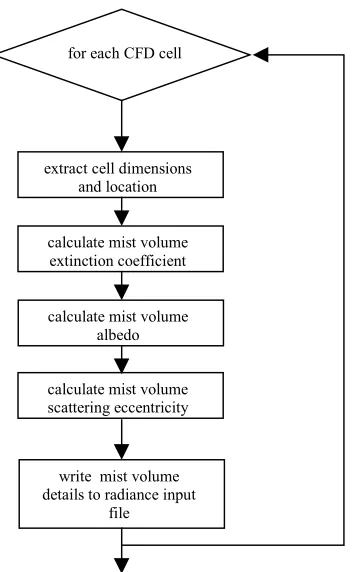
The model parameters, together with the dimensions of each CFD cell are used to build a model for the Radiance simulation. In this model each CFD cell is converted to a volume of “mist” in the Radiance model, with the appropriate extinction coefficient, albedo and scattering eccentricity. This produces a 3-D image of the non-homogeneous, droplet distribution corresponding to that produced by the CFD model. The algorithm for the conversion process is shown in figure 4.

EXAMPLE – FOG PRODUCTION

Figures 5-7 show output from ESP-r’s CFD tool and Radiance depicting the production of fog in a small test room, with four nozzles at the ceiling spray droplets into the space.

Figure 4 is a montage of various 2-D slices through the CFD domain showing the droplet concentration and shows four dense columns of droplets below the nozzles. The droplet concentration distribution is then converted to a radiance input file within the CFD code, which is then passed to radiance for processing.

for each CFD cell

extract cell dimensions and location

calculate mist volume extinction coefficient

calculate mist volume albedo

calculate mist volume scattering eccentricity

write mist volume details to radiance input

file

Figure 4 CFD to Radiance data transfer.

Figures 6 and 7 show the impact of fog production the droplets in the climate room. Figure 5 shows the space with no droplets, while figure 6 shows the columns of droplets below the spraying nozzles, as evident in the CFD output.

OTHER USES

There are numerous potential applications for the software developed during this project. These include:

use of the droplet model of the CFD tool to

model particulate contaminant dispersal in buildings, including smoke, dust, etc;

use of the CFD-Radiance link to model smoke

filled environments (e.g. the simulation of the effectiveness of fire safety signs);

application of the lighting simulation

component in the field of driving safety (e.g. collision detection) and driving simulation.

WORK-TO-DO

The work presented here is very much a first attempt at a linkage between CFD and Lighting simulation.

More research is required in several areas:

further improvement and verification of the

CFD small-particle continuum model;

determination of scattering eccentricities for different small-particle types;

optimisation in the rendering of large numbers of finite ‘fog’ or particle volumes: currently a single image takes more than 24 hours to produce;

verification of radiance simulation output.

CONCLUSIONS

The work presented here represents a novel linkage between two hereto disparate domains of simulation: lighting simulation and CFD. The linkage was developed for a very specific application: the visualisation of artificial fog production in a climate chamber.

In this work an attempt is made to model both the thermodynamic and optical reality through modelling the droplet transport and concentration distribution using CFD and then modelling the resulting 3-D visual domain using Radiance. In other visualisations (e.g. simulators and games) no attempt is made to realistically model physical reality.

The principles presented in this paper can be applied to other cases of small particles suspended in air including fog, smoke and dust. Hence, combined CFD-lighting simulations could have significant potential applications in both fire and automotive safety.

REFERENCES

[1] Clarke J A, Energy Simulation in Building Design 2nd Ed. Butterworth-Heinemann Publishers, 2001.

[2] Larson G W, Shakespeare R A, Rendering with Radiance: The Art and Science of Lighting Simulation, Morgan Kauffman Publishers, 1998.

[4] Silva C A and Hannay J, 2001. Presentation to Glasgow Meeting, 2001 in Proc. of the Third Working Meeting Growth Contract No. G6RD-CT-2000-0211, Glasgow, May 2001.

Figure 5 composite image showing CFD results from which the Radiance images are derived.

Figure 6 No mist in the test room Figure 7 Non-homogeneous mist in the test room,