CONTROLLER PERFORMANCE DESIGN AND
ASSESSMENT USING NONLINEAR GENERALIZED
MINIMUM VARIANCE BENCHMARK: SCALAR CASE
P. Majecki*
†, M.J. Grimble*
*The University of Strathclyde, 50 George Street, Glasgow G1 1QE, UK
†Corresponding author: [email protected], fax 0141 5484203
Keywords: Nonlinear control, Optimal control, Controller performance assessment.
Abstract
A nonlinear version of the Generalized Minimum Variance (GMV) multivariable control law has been recently derived for the control of nonlinear, possibly time-varying systems. This paper presents the results of the controller performance assessment against this Nonlinear GMV controller in the scalar case. The minimum variance of the generalized output is estimated from routine operating data given only the plant time delay and the technique is applied to a nonlinear reactor control example.
1 Introduction
Minimum variance (MV) criteria have been used in stochastic performance assessment since the subject of control loop benchmarking was introduced by Harris [7]. The later research by Desborough and Harris [3] and Stanfelj et al. [10] built on this work, showing how time-series analysis can be used to estimate the minimum achievable variance of the controlled variable from routine operating data, and defining the ''controller performance index'' as the ratio of this minimum variance to the actual variance. This early work was focused mostly on assessing SISO LTI control loops against the MV benchmark.
The ''Generalized Minimum Variance'' criterion (derived by Clarke and Hastings-James [1,2] and re-derived by Grimble [4] using an unconditional cost function) addressed some of the problems related with the MV control (aggressive control action, poor robustness) by considering a combination of the weighted error and control signals. The GMV benchmarking results for the scalar case were presented by Grimble [5].
Grimble [6] has recently introduced a GMV controller for nonlinear processes. When the system is linear the results revert to those for the linear GMV controller, and this suggests that the algorithms used for benchmarking linear controllers might also be applicable to the nonlinear case. Since the benchmarking data-driven techniques have so far been limited to the assessment against optimal linear controllers, this would be a significant advance, achieved with
little extra cost. The aim of the following is therefore to investigate this possibility.
2 Stochastic system description and NGMV
performance criterion
The system shown in Fig. 1 is of restricted generality and is carefully chosen so that simple results are obtained. The plant itself is nonlinear and may have quite a general form which might involve state-space, transfer operators, neural networks or even nonlinear function look-up tables. However, the reference and disturbance signals are assumed to have linear time-invariant model representations. This is not very restrictive, since in many applications the models for the disturbance and reference signals are only LTI approximations.
A nonlinear plant model can be written in the following form:
(
)( )
k(
)( )
k
u t =z− u t
W W , (1)
where k denotes the magnitude of the plant time-delay.
2.1 Signals
The signals shown in the system model of Fig. 1 may be listed as follows:
Error signal: e t
( ) ( ) ( )
=r t −y t (2) Plant output: y t( ) (
=W
u t)( )
+d t( )
(3) Reference: r t( )
=Wrζ
( )
t (4) Disturbance signal: d t( )
=Wdξ
( )
t (5) The power spectrum for the combined reference and disturbance signal f = −r d can be computed as:* *
ff rr dd r r d d
Ф =Ф +Ф =W W +W W (6) and the strictly minimum phase generalized spectral-factor Yf
may be computed using: *
f f ff
Y Y =Ф . (7)
2.2 NGMV cost function
The optimal NGMV control problem involves the minimisation of the variance of the signal
φ
0( )
t in Fig. 1. This signal involves a dynamic cost function weighting1
( )
c
P z− on the error signal, represented in transfer-function
form as: c cn
cd
P P
P
= . It also includes a nonlinear dynamic
control signal costing operator term:
(
F
cu t)( )
. The choice of the dynamic weightings is critical to the design and typically Pc is low-pass andF
c is a high-pass transfer. The signal:( )
(
)( )
( )t P e tc cu t
φ
= +F
(8)is to be minimized in a variance sense, so that the cost index to be minimised:
( )
{ }
2J =E
φ
t . (9)If the plant time-delay is of magnitude k, this implies the control at time t affects the output k steps later. For this reason the control weighting can be defined as:
(
F
cu t)( )
=z−k(
F
cku t)( )
(10) Typically this will be a linear operator but it may also be chosen to be nonlinear to compensate for the plant input nonlinearities in appropriate cases. The control weighting operatorF
ck is assumed to be invertible.Pc
Wr
Wd
r + e u -
y d
W +
+ m
Fc Disturbancemodel
Control weighting
Reference Error weighting
+ + ξ
C0
Nonlinear plant Controller
c c
P e u φ = +F
ζ
Fig.1: Single Degree of Freedom Feedback Control System for the Nonlinear Plant (inferred output φ0 is dependent on
the weightings shown dotted)
2.3 Generalized plant
One approach to the above control problem is to reformulate the GMV criterion as a simpler minimum variance problem for a generalized plant. The expression for the controller error can be written as:
(
)( )
( ) k k f ( )
e t = −z− Wu t +Y
ε
t (11) where ε(t) is a zero-mean, unity-variance white noise and Yfrepresents the combined effect of all the stochastic inputs to the system.
The generalized output
φ
( )
t can be rewritten as follows:(
)( )
(
)( )
( )
( ) ( ( ))
( ) ( )
k
c k f c
k
ck c k c f
t P z u t Y t u t z P u t P Y t
φ
ε
ε
−
−
= − + +
= − +
W F
F W (12)
Notice that the non-linear operator in this last expression can be considered a “generalized plant” and the notation implies that:
(
PcW
−F
c)
u P= c(
W
u t)( )
−(
F
cu t)( )
(13)3 Optimal Nonlinear GMV Problem and
Solution
The key step in the derivation of the NGMV control law is to split the cost function (9) into two statistically non-overlapping terms, one of which is independent of, and the other dependent on the controller. The control law then results by simply setting that second term to zero.
Splitting the weighted disturbance term into unpredictable and predictable components using the Diophantine identity (deg F < k):
k c f
PY
= +
F z R
− , (14)equation (16) can be rewritten as:
( )
( )t F t( ) z k ( ck Pc k)u t R t( )
φ
=ε
+ − ⎡ − +ε
⎤⎣ F W ⎦ (15)
To compute the optimal control signal, inspect the form of equation (15). Since the degree of Fis required to be less than k, it follows that the first and the remaining terms are statistically independent, even though the second term involves a nonlinear operator.
Furthermore, the first term on the right of (15) is independent of the control action and the smallest variance is achieved when the remaining terms are set to zero. The optimal control signal must therefore satisfy:
1
( ) ( ) ( )
opt
ck c k
u t = − F −PW − R t
ε
(16) which after some manipulations can be rewritten as1 1 1
( ) [( ) ]( )
opt
ck f k f
u t = − F −FY−W − RY e t− (17) The above result indicates that the restriction on the choice of the cost weightings is that the operator
(
PcW
k −F
ck)
must have a stable inverse.The generalized output under NGMV optimal control is a linear moving-average time series:
( ) ( )
opt t F t
φ
=ε
. (18)Its variance (the minimum value of the cost function) follows as:
[
]
1 2min
0
( )
k ii
J
Var F t
ε
−f
=
=
=
∑
(19)3.1 Selection of the dynamic weightings
Since the properties of the benchmark controller depend on the choice of the dynamic weightings, some guidelines are needed to help in their selection. The weightings should ideally reflect the requirements imposed on the control system (good regulatory and tracking performance, load rejection, robustness) and these are normally process-dependent. Some rules of thumb, however, can be given for the linear case and may be used as a starting point for the design.
In general, the frequency dependence of the weightings can be used to weight different frequency ranges in the error and control signals. The error weighting Pc should typically
include an integrator, which leads to integral action in the controller, and the control weighting is chosen as a constant or as a lead term to ensure the controller rolls-off in high frequencies and does not amplify the measurement noise. An additional scalar may be used to balance the steady-state variances of the error and control signals.
As shown in [6], if a controller Kc exists that stabilizes the
delay-free plant, then a choice of weightings leading to a stabilizing NGMV controller can be defined as Pc=Kc and
1
ck = −
F
. This selection can therefore provide a starting point for the design.4 Estimation of the Controller Performance
Index from routine operating data
In this section two data-driven estimation algorithms are reviewed which have received considerable attention in the literature on the benchmarking of linear control systems. The objective is to estimate the theoretically achievable lower bound on the value of the NGMV cost function (9) from routine closed-loop operating data.
4.1 Harris algorithm
This approach was first introduced in the seminal papers ([7],[3]) and subsequently referred to by many authors as the ‘Harris algorithm’. In this approach, an autoregressive time series model is fitted to the filtered and detrended data:
0
( )
( )
i(
)
i
t
F t
t k i
φ
ε
∞α φ
=
=
+
∑
− −
(20)The infinite sum is approximated by truncating to m terms and the α coefficients are estimated using least squares. The data may be written in vector-matrix form as:
X
φ
=
α ε
+
(21)and, assuming X is invertible, the vector of autoregressive parameters is then found as:
1
(
X X
T)
X
Tα
=
−φ
Finally the minimum variance estimate follows as the residual error variance:
2
1
ˆ
(
) (
)
2
1
T
mv
X
X
N k
m
σ
=
φ
−
α φ
−
α
− −
+
(22)where N is the data ensemble length.
4.2 FCOR algorithm
The idea behind this algorithm, which was introduced in [8], is to directly estimate the coefficients of the polynomial F. This can be done by cross-correlating the generalized output φt with the estimated white noise input to the system (signal εt
in (15)), as outlined below.
The algorithm consists of two main steps: (a) Whitening process.
The detrended generalized output φt is modelled as an
autoregressive time series and then filtered to obtain the white noise ‘innovations’ sequence:
1 1
1
(
)
(
)
t t t
A q
tA q
φ
ε
ε
−φ
−
=
⇒
=
(23)(b) Computing the cross-correlation between the output and the estimated noise:
( )
[
t t i]
i,
0
1
r i
φε=
E
φ ε
−=
f
i
=
…
k
−
(24)where the white process εt has unity variance. The right-hand
sides follow from equation (15), and the coefficients of the polynomial F are thus determined. The minimum achievable variance follows from (19).
4.3 Controller Performance Index
The controller performance index (CPI) is defined to be the ratio of the minimum variance of the signal
φ
to the actual variance. That is, the CPI can be obtained asmin
J
J
κ
=
(25)where Jmin is the minimum value of the cost function (9) and J
is the actual value. Clearly,
0
≤ ≤
κ
1
, with ‘1’ indicating the best possible performance and no opportunity for improvement by tuning the controller. If on the other hand the CPI indicator κ is close to zero then retuning may be recommended. The above scalar is well-known in controller benchmarking as the ‘Harris index’.4.4 Remarks
As can be seen from equation (19), the minimum achievable variance does not depend on the control weighting. This suggests that the above estimation algorithms can be applied to the weighted error signal rather than to the full generalized output.
The above algorithms were presented as for the linear case, however, they can be used for nonlinear GMV benchmarking without any modifications other than a possible use of a nonlinear control weighting (and in view of the previous remark, this just to estimate the actual output variance). The assumption here is that the nonlinear character of the signal can be adequately captured by a linear time-series model.
5 Simulation example
The example comes from [9] and involves a model of a simple chemical process. The process is an irreversible exothermic first order reaction, which takes place in a continuous stirred tank reactor (CSTR).
Fig. 2. CSTR process
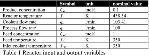
[image:4.595.309.525.85.259.2]The input and output process variables are summarised in Table 1. It is assumed that:
- the liquid in the reactor is perfectly mixed - the feed flow is equal to the product outflow.
Symbol unit nominal value
Product concentration Ca mol/l 0.1
Reactor temperature T K 438.54 Coolant flow rate qc l/min 103.41
Process flow rate q l/min 100 Feed concentration Ca0 mol/l 1
Feed temperature T0 K 350
[image:4.595.44.255.247.400.2]Inlet coolant temperature Tc0 K 350 Table 1 Reactor input and output variables
For the purpose of our example, the behaviour of the CSTR process is considered about a set-point where the concentration of the product stream is 0.1 mol/l. The coolant flow rate qc [l/min] is regarded as an input to the process and
the product concentration Ca [mol/l] is regarded as the output.
The CSTR process exhibits some rich non-linear behaviour. It has multiple steady-state solutions and it shows a clearly non-linear dynamic response. While for small excursions about a nominal working point a linear model may be sufficient to describe the behaviour of the process, a nonlinear model is preferred over larger ranges. The open-loop step responses for both the nonlinear model and the model linearised around the nominal operating point are shown in Fig. 3.
0 10 20 30 40 50 60 70 80 90
0.09 0.095 0.1 0.105 0.11 0.115
Small deviations
C
a
[m
o
l/
l]
Linear model Nonlinear model
0 10 20 30 40 50 60 70 80 90
0.06 0.08 0.1 0.12 0.14 0.16
Large deviations
C
a
[m
o
l/l
]
time [min]
Linear model Nonlinear model
a b
a
[image:4.595.38.285.469.560.2]b
Fig. 3. Open-loop step responses: (a) Linear model, (b) Nonlinear model
5.1 NGMV Controller Design
The linearised model obtained in the previous subsection was first used to design a linear GMV controller. The disturbance
model was chosen as
0.001
11 0.95
d
W
z
−=
−
.The reference model has been assumed zero, however the integral action will be introduced to the controller through the error weighting.
Two choices of dynamic weightings have been considered: (i) derived directly from the existing PI design:
1 1
1
14(1 0.5
)
1
c
z
P
z
−−
−
=
−
,1
1
ck
F
= −
(ii) based on the frequency-domain rules of thumb: 1
2
1
1 0.85
1
c
z
P
z
−−
−
=
−
,2
0.015(1 0.1
1)
ckF
= −
−
z
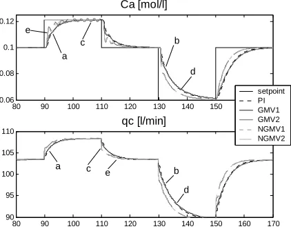
−Both sets of weightings have also been used to design the nonlinear controllers NGMV1 and NGMV2. The simulation results in Fig. 4 show the transient performance with all the above controllers in the feedback loop (without noise) for ‘large’ deviations from the nominal set-point.
5.2 Estimation of the Controller Performance Index
For the stochastic performance analysis we will consider only the second set of weightings (i.e. the controllers GMV2 and NGMV2). A new simulation experiment was performed to obtain a set of noisy data. The error and control data were then filtered to create the generalized output φ(t) and both the Harris and the FCOR algorithms were applied to this signal. Finally the benchmark costs have been evaluated and the controller performance index (CPI) calculated using expression (25). The benchmarking results for three operating points are presented in Table 2. The figures correspond to the FCOR algorithm but those obtained from the Harris algorithm were almost identical.
q, T0, Ca0
q, T, Ca
qc, Tc0
T, Ca
80 90 100 110 120 130 140 150 160 170 0.06
0.08 0.1 0.12
Ca [mol/l]
80 90 100 110 120 130 140 150 160 170
90 95 100 105 110
qc [l/min]
setpoint PI GMV1 GMV2 NGMV1 NGMV2
a
b c
d e
c
a b
[image:5.595.307.513.82.131.2]d e
Fig. 4. Transient responses – ‘large’ deviations (a) PI, (b) GMV1, (c) GMV2, (d) NGMV1, (e) NGMV2
5.3 Comments on the results
The results confirm the better performance of the nonlinear GMV controller over the whole operating range. While the linear GMV control is adequate for small deviations from the nominal operating point, its performance degrades away from it (compared with the nonlinear control). This is especially true for higher values of the product concentration Ca, where
the nonlinearity becomes significant, and is less noticeable for smaller values where the main difference between the linear and nonlinear model is the steady-state offset.
Both estimation algorithms have proved to be able to return the minimum variance estimates close to the true value. The accuracy could be still increased by increasing the data length, the model length, or averaging over a number of realizations.
The performance indices confirm the above comments – the NGMV index is close to 1 across the operating range, while the performance of the linear GMV controller drops significantly for the higher operating region. The PI index seems to be relatively robust and its value suggests the possibility of improving the stochastic performance of the system. The robustness of this simple controller can also be seen from the transient (noiseless) responses, where its performance is comparable to the other optimal controllers.
Overall the transient performance of all considered controllers is comparable. From the plots (Fig 4) it can only be seen that the controllers GMV2 and NGMV2 have faster transients due to greater bandwidth and that the linear controller GMV2 is close to becoming unstable for the higher operating region. The PI-based controllers GMV1 and NGMV1 stay close to the PI, as it is usually the case.
Op. point PI GMV2 NGMV2
[image:5.595.62.273.85.251.2]0.06 0.143 0.927 0.998 0.1 0.227 0.998 0.998 0.12 0.269 0.333 0.995 Table 2. Estimated Controller Performance Index
6 Conclusion
Design and performance assessment against a relatively simple controller for nonlinear systems was considered.
The example demonstrated the potential benefits that can be gained by using the nonlinear controller – these benefits depend upon the system nonlinearities and the potential improvement is the greater the bigger control problems are caused by these nonlinearities. The benefits that can be gained by using the nonlinear GMV control can be assessed by using the benchmarking techniques. Two such techniques have been reviewed and used to estimate the controller performance index.
Acknowledgements
This work was supported by EPSRC Grant GR/R65800/01. The authors are grateful to Dr. Leonardo Giovanini for providing the reactor model and to Dr. Andrzej Ordys for helpful discussions.
References
[1] Clarke D.W., Hastings-James R., 1971, “Design of digital controllers for randomly disturbed systems”, Proceedings of IEE, Vol. 118, No. 10, 1503-6
[2] Clarke, D W, and Gawthrop, P J, 1975, Self-tuning controllers, Proc IEE, Vol 122, No 9, pp 929- 934.
[3] Desborough L.D. and Harris T.J., 1992, "Performance assessment measures for univariate feedback control", The Canadian Journal of Chemical Engineering, Vol. 70, p. 1186-1197
[4] Grimble M.J., 1988, “Generalized Minimum Variance Control Law Revisited”, Optimal Control Applications & Methods, Vol. 9, 63-77 [5] Grimble M.J., 2002a, “Controller Performance Benchmarking and
Tuning using Generalized Minimum Variance Control”, Automatica, Vol. 38, p.2111-2119
[6] Grimble M.J., 2003, “Generalized Minimum Variance Control of Nonlinear Multivariable Systems”, Submitted to the IEE Proceedings, Control Theory and Applications
[7] Harris T.J., 1989, “Assessment of control loop performance”, The Canadian Journal of Chemical Engineering, Vol. 67(10), p. 856-861. [8] Huang B. and S.L.Shah, 1999, “Performance assessment of control
loops: Theory and Applications”, Springer Verlag. London
[9] Morningred, D., B. Paden & D. Mellichamp, 1992, "An adaptive nonlinear predictive controller", Chem Eng. Sci, Vol 47, pp. 755-765. [10] Stanfelj N., Marlin T.E., MacGregor J.F., 1996, “Monitoring and