Spatial Ecology of Adelie Penguin Breeding
Colonies:
The Effects of Landscape, Environmental
Variability and Human Activities
by
Phillippa Kate Bricher B.A., Grad. Cert. GIS.
(University of Tasmania)
Declaration
This thesis contains no material which has been accepted for the award of any other degree or diploma in any tertiary institution, and to the best of my knowledge and belief, contains no material previously published or written by another person, except where due reference is made in the text of the thesis.
Signed
Abstract
Adelie penguins have been widely studied as an "indicator" species for the health of the Southern Ocean ecosystem. However, the effects of climatic variability and human activities on Adelie penguin populations are poorly understood. As many of the Adelie penguin colonies used for long-term demographic studies are located near research stations, there is a need to be able to disentangle the effects of human activities and environmental variability on Adelie penguin populations. This study investigates the landscape properties that drive the locations of Adelie penguin colonies in the Windmill Is, East Antarctica. It also examines whether potential changes in snow cover and/or proximity to human activities best explain the varying population trends of colonies in two breeding localities. While some colonies have been abandoned, or have undergone strong population decreases, the populations of others have grown by more than 1000% in the past 38 years.
This study uses Geographic Information Systems to generate spatial data of landscape, snow accumulation patterns and proximity to human activity parameters. Landscape parameters are derived from fine-scale digital elevation models (DEMs) and snow accumulation patterns are modelled using a complex physically-based GIS model. The parameters are then combined into multivariate statistical models to generate predictions of habitat suitability.
Individually, the landscape attributes, such as elevation, slope, solar radiation, and wetness index, have little power to predict the distribution of colonies within a breeding locality. On the• other hand, multivariate models (discriminant analysis and decision tree) derived from these landscape attributes predict the presence or absence of colonies in test grid cells with up to 78.9% accuracy. General rules to describe the distribution of Adelie penguin colonies are not easily derived, as habitat suitability appears to be driven by complex interactions between landscape attributes.
Acknowledgments
This study would not have happened without my two dedicated, passionate and patient supervisors — Dr Arko Lucieer and Dr Eric Woehler. This thesis has greatly benefited from Arko's gentle encouragement, answers to an endless string of questions and excellent problem solving skills. Without Eric, the project would never have started. I'd like to thank him for taking me to Antarctica in the first place, and for a thousand explanations and corrections.
I'd like to thank all members of the 59th ANARE to Casey, especially the volunteer penguin counters, the dive team's water taxi service and the station leader, Marilyn Boydell, for facilitating my fieldwork.
The Australian Antarctic Data Centre played an invaluable role by providing me with data, equipment and advice and by answering all my questions. Dr Ben Raymond's statistical expertise and teaching helped enormously with designing the project and with interpreting the results.
At the University of Tasmania's School of Geography and Environmental Studies, the support of several colleagues is gratefully acknowledged. Mr Rob Anders' efforts to generate the photogrammetric DEMs, despite less than ideal photographs and ground control data made this project possible and proved to be character-building for us both. Many thanks also to Dr Jon Osborn for his unstinting support and advice on the photogrammetric aspects of the study. Dr Neil Adams (IASOS) was outstandingly kind in speedily providing me with data and advice on how to use the NCEP/NCAR weather reanalysis data. Peter Morgan gathered vital ground control data at short notice. In addition, there were numerous hallway conversations throughout the year with staff and fellow students that produced new insights. Thanks to Gary Sjoberg (Flinders University) for his lessons on formatting large and unwieldy documents.
Finally, thanks go to my parents for their belief and support.
Some or all of the data used within this paper was obtained from the Australian Antarctic Data Centre (IDN Node AMD/AU), a part of the Australian Government Antarctic Division (Commonwealth of Australia). The data is described in the following metadata records:
"Windmill Islands 1:50000 GIS Dataset" Ryan, U. (1999, updated 2006).
Contents
Declaration Abstract
Acknowledgments • 1 Introduction
ii
iv
1
1.1 Climate variability and Adelie penguin populations 1
1.2 Human impacts and Adelie penguins 2
1.3 The role of GIS in studying these phenomena 3
1.4 Adelie penguins 4
1.5 Definitions 5
1.6 Aims and objectives 8
1.7 Hypotheses 8
2 Literature Review 10
2.1 Spatial ecology of Adelie penguins and the effects of landscape processes 10
2.1.1 Adelie penguin distribution 10
2.1.2 Coloniality 11
2.1.3 Topographic influences on colony locations 12
2.1.4 Climate variability and snow accumulation 15
2.1.5 Human impacts on Adelie penguins 16
2.2 GIS habitat modelling 19
2.3..1 Univariate testing
2.3.2 Multivariate model selection 24
2.3.3 Model refinement 26
2.3.4 Testing validity 26
2.4 Snow accumulation modelling 27
2.4.1 Snow transport mechanisms 27
2.4.2 Why snow accumulation is modelled 28
2.4.3 Available snow accumulation models 28
2.4.4 Commonly used physical inputs 32
3 Chapter 3: Data and Methods 34
3.1 3.1 Study areas 34
3.1.1 Windmill Is 34
3.1.2 Geology • 34
3.1.3 Weather 36
3.1.4 Human history 36
3.1.5 Shirley I 36
3.1.6 Whitney Pt 37
3.2 Data sets 39
3.2.1 Adelie penguin counts 39
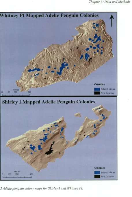
3.2.2 Adelie penguin colony maps 39
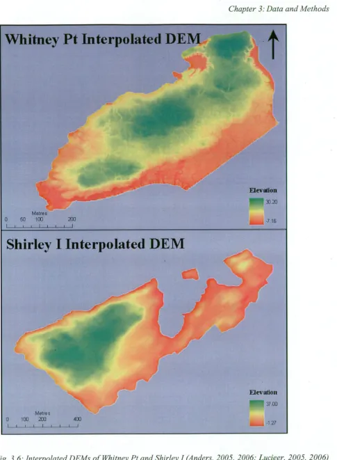
3.2.5 Digital elevation models 45
3.2.6 NCEP/NCAR Weather reanalysis data 49
3.3 Methods 50
3.3.1 GIS processing methods 50
3.3.2 Statistical Processing Methods 62
4 Results 69
4.1 GIS landscape layers 69
4.1.1 Slope 69
4.1.2 Aspect 69
4.1.3 Wetness index 69
4.1.4 Solar radiation 69
4.1.5 Planar and profile curvatures 70
4.1.6 Surface roughness 70
4.1.7 Adjacency 70
• 4.1.8 Wind exposure 70
4.1.9 Snow accumulation model 70
4.1.10 Proximity to Human Activities 71
• 4.1.11 Population trends • 71
4.1.12 Summary Statistics 72
4.2.1 Univariate Analyses
4.2.2 Discriminant Analyses 83
4.2.2.1 Whitney Pt 83
4.2.3 Decision Tree Analyses 91
4.3 Snow Accumulation Patterns and Adelie Penguin Colony Population Trends 94
4.3.1 Univatiate Analyses 94
4.3.2 Discriminant Analyses 96
4.3.3 Decision Tree Analysis 105
4.4 Proximity to human activities and population trends of Adelie penguin colonies 108
4.4.1 Univariate Analyses 108
4.4.2 Discriminant Analyses 110
4.4.3 Decision Tree Analyses 118
5 Discussion 121
5.1 The effect of landscape on Adelie penguin distribution in the Windmill Is 121 5.2 The effect of snow accumulation patterns on Adelie penguin colony population trends in the
Windmill Is 123
5.3 The effect of proximity to human activities on Adelie penguin colony population trends in the
Windmill Is 124
5.4 How this study compares with other GIS-based habitat analyses 127
5.5 Limitations on the study 129
6 Conclusions 132
Appendix 1: Summary Statistics 147
Summary statistics for Whitney Pt Addle penguin colony distribution 147 Summary- statistics for Shirley I Adelie penguin colony distribution 148 Summary statistics for Whitney Pt Adelie penguin colony population trend classes 149 Summary statistics for Shirley I Adelie penguin colony population trend classes 151
Appendix 2: Discriminant Analysis Formulae 153
Adelie penguin colony distribution models: 153
Whitney Pt 153
Shirley I 155
Snow accumulation patterns and Adelie penguin colony population trends 158
Whitney Pt 158
Shirley I 159
Proximity to human activities and population trends of Adelie penguin colonies 161
Whitney Pt 161
Shirley I 164
Appendix 3 Decision Trees 167
Adelie penguin colony distributions 167
Whitney Pt 167
Shirley I 168
Whitney Pt
Shirley I 169
Proximity to human activities and population trends of Adelie penguin colonies 172
Whitney Pt 172
I Introduction
The effect of climate change on the environment is an issue of current public and scientific concern. Some of the most significant climate alterations have been observed in polar regions (e.g. Fraser and Patterson, 1997; Croxall. et al., 2002; Ainley, 2002; Forcada et al., 2006). In addition, Antarctica is designated as a wilderness zone to be protected under the Antarctic Treaty. Therefore, an understanding of the effects of climate change is particularly critical for management of Antarctic environments.
Seabirds have been widely used as indicators of changes in the Southern Ocean ecosystem (e.g. Micol and Jouventin, 2001; Croxall et al., 2002; Kato et al., 2002; Kato et al., 2004). There are a number of reasons for this, including their perceived primary role in the Southern Ocean ecosystem and the ease with which they can be monitored (Micol and Jouventin, 2001; Kato et al., 2002). However, it has also been acknowledged that using birds as bioindicators of climate change is problematic because of the complex nature of the numerous interactions in the Southern Ocean ecosystem (Croxall et al., 2002) and the potential confounding effects of human impacts at local scales. Adelie penguin (Pygoscelis adeliae) colonies are known to be abandoned and recolonised as the climate changes (Ainley, 2002; Emslie and Woehler, 2005) and have hence been termed "bellwethers of climate change" (Ainley, 2002).
1.1 Climate variability and Adelie penguin populations
The localities used by breeding Adelie penguins are affected by interactions between the terrain and local climatic conditions. One of the key facets of this study is the investigation of the impact of snow accumulation on the distribution of colonies and on their population trends over 46 years. One previous study attempted similar analyses (Fraser and Patterson, 1997). That study used a hillshade model as a surrogate for wind exposure to penguin colonies. Wind exposure was, in turn, used as an indicator for areas where snow would be abraded. The present study applies a more complex snow accumulation model, based on the physics of drifting snow and available meteorological data (Wallace, 2005).
effects of climate changes and human activities (e.g. Fraser and Patterson, 1997; Micol and Jouventin, 2001). The present study followed the latter approach, and attempts to differentiate between climatic and human-induced effects.
Many studies of the effects of climatic variation on Adelie penguin population trends have focused on broader-scale variables, such as sea-ice extent. These studies have generated somewhat contradictory results. There is debate about the extent to which these studies have been able to show clear patterns or causal mechanisms for population fluctuations (Croxall et al., 2002; Ainley et al., 2003). It is possible that part of the reason for these contradictory results is that other environmental factors are confounding or exacerbating the effects of sea-ice changes at different sites and in different years (Fraser and Trivelpiece, 1996; Fraser and Patterson, 1997; Ainley et al., 2003). This study attempts to increase understanding of local environmental effects that alter the suitability of individual colony sites. This will, in turn, improve the interpretation of local, regional and ecosystem-scale population trends.
1.2 Human impacts and Adelie penguins
Human activities have had substantial impacts on the physical environment of Antarctic coastal areas (e.g. Young, 1990; Wilson et al., 1990; Micol and Jouventin, 2000.. For Adelie penguins, this effect has been most severe where penguin colonies have been destroyed for the construction of research stations and associated infrastructure (Wilson et al., 1990; Micol and Jouventin, 2001). There is argument about the potential impact of human activities outside the immediate footprint of research stations (Wilson et al; 1989; Culik et al., 1990; Wilson et al., 1991; Woehler et al., 1994; Giese, 1996; Fraser and Patterson, 1997; Micol and Jouventin, 2001; Pfeiffer and Peter, 2004). Woehler et al. (1994) proposed that decreasing populations in some penguin colonies were the result of pedestrian visits by station personnel.
Peter, 2004). However, it is also potentially an issue around all Antarctic research stations. Long-term studies of Adelie penguin populations have typically been generally conducted near research stations, where human activities are focused (e.g. Woehler et al., 1994; Fraser and Patterson, 1997; Micol and Jouventin, 2001; Woehler et al., 2001). Studies of Adelie penguins have also generally involved nesting birds. This means that it may be difficult to disentangle any effects of climatic variability and the role of human activities on numbers of breeding Adelie penguins. Clarke and Kerry (1994) raised concerns about the effects of invasive monitoring procedures on the validity of scientific observations of Adelie penguins at Bechervaise Island, near Mawson.
1.3 The role of GIS in studying these phenomena
In recent years, Geographic Information Systems (GIS) have been used extensively for habitat analysis of plant and animal species across the globe (e.g. Glenz et al., 1991; Manel et al., 1999; Lenton et al., 2000), as the development of GIS software has made it possible to include spatial variability data into ecological studies (Maurer, 1994). However, GIS has rarely been used to examine the land-based habitat requirements of Adelie penguins, with the exception of Fraser and Patterson (1997). Historically, attempts to study the nest-site requirements of Adelie penguins have been forced to ignore the spatial variability of terrain in and among colonies. This was largely because of the inability of available analytical techniques and computing power to adequately examine spatial data (Yeates, 1975; Moczydlowski, 1986 and 1989; Maurer, 1994; Evans, 1991). Some studies of human impacts have incorporated some limited assessment of the spatial variability of human activities (e.g. Wilson et al., 1990; Young, 1990; Woehler et al.,
1994; Fraser and Patterson, 1997; Patterson et al., 2003).
assessment and quantification of the spatial variability of nesting sites (Yeates, 1968; Moczydlowski, 1986, 1989).
Historically, most studies have looked at population trends for what are here termed breeding localities — areas that contain several colonies (using the definition of Woehler et al. (1991, 1994). There has been little examination of the spatial variability of demographic data within breeding localities. Exceptions to this include Woehler et al. (1994) who reported correlations between the population trends of colonies and their distance from Casey, Fraser and Patterson (1997) who compared the role of variability in wind exposure with the population trends of colonies, Wilson et al. (1990) who investigated the effects of human disturbance associated with the Cape Hallett research station on penguin breeding success and Patterson et al. (2003) who examined the relationships between snow accumulation, tourist visits and colony population trends.
In the Windmill Is, individual Adelie penguin colonies have exhibited different population trends. Several of the colonies closest to Casey have undergone population decreases during the 50 years of human occupation in the Windmill Is region (Woehler et al., 1994; E.J. Woehler, unpub. data). However, the overall Adelie penguin population of the Windmill Is trebled between 1961/62 and 1989/90, with the populations of many colonies increasing, and new colonies established at many breeding localities (Woehler et al., 1991). This trend has continued to the present (E.J. Woehler, unpub.. data). An analysis of fine-scale processes is needed to contribute to our understanding of the observed variability:
1.4 Adelie penguins
Wilson's storm-petrels (Oceanites oceanicus).
One of the advantages in studying the distribution of Adelie penguins is that their current and former spatial distributions can be easily mapped. The birds form colonies of up to thousands of pairs. Adults build nests from small pebbles, collected from surrounding areas, to raise their eggs/chicks above the ground and so protect them from snow and meltwater (Ainley, 2002). In the Windmill Islands, these accumulations of nest pebbles have been shown to be up to 9000 years old (Emslie and Woehler, 2005). The perimeters of existing and former colonies can be clearly seen in aerial photographs and on the ground.
Regional trends have been identified in Adelie penguin populations across Antarctica. East Antarctic populations have shown sustained increases; populations on the Antarctic Peninsula have increased and decreased, and those in the Ross Sea showed no clear pattern (Woehler and Croxall, 1998; Woehler et al., 2001). Most population studies have examined regional trends, and there is a need for better understanding of finer-scale variation within regions.
Adelie penguins can feed a considerable distance out to sea. A tracking study at Shirley I, near Casey, found that breeding penguins travelled between 31 and 144 kilometres from the colony (Wienecke et al., 2000). Another study of the foraging range of penguins at Shirley I found that they had a maximum foraging range of 135 kilometres (Kerry et al., 1997). These findings are broadly consistent with studies in other parts of the continent which have found that Adelie penguins feed between 2 and 100 kilometres from the colonies, with the short distances associated with extensive fast-ice (e.g. Kerry et al., 1995; Watanuki et al., 1997; Ainley, 2002). Given the large distances Adelie penguins travel to feed, and the short distances between colonies within a breeding locality, it is considered that land-based influences on Adelie penguin colonies are more likely to explain population trend differences among colonies than differences in the marine environment.
1.5 Definitions
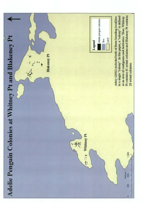
groups of birds should be described as discrete colonies depends on the degree of interaction among the groups. This study uses the definitions in Woehler et al. (1991) and Woehler et al. (1994): A breeding colony is here defined as an area of contiguous nest territories. In turn, a nest territory is defined as an area containing a nest, and which is defended by a breeding pair, and is typically approximately 1 m2 . A breeding locality is a geographical feature, either an island or a discrete area of mainland, on which breeding colonies are found. Thus, Whitney Pt contains 48 colonies (sensu Woehler) and is considered to be one breeding locality. This contrasts with the definition of Ainley (2002) who used the term "colony" for what is here termed a breeding locality (Fig. 1.1), and with the term "rookery" which was historically used to describe breeding localities (e.g. Penney, 1968).
Sites that contain conspicuous and clearly outlined agglomerations of nest pebbles, and are not known to have been used by breeding pairs of penguins during the period of human occupation in Antarctica have often been described as "relict" colonies (e.g. Penney, 1968; Woehler et al., 1994; Emslie and Woehler, 2005). This study follows that definition, but uses the term "relic" rather than "relict" to refer to these unused colonies. This change follows the Oxford • Dictionary's (Pearsall, 1999) definitions as follows:
"Relic n. 1 an object of interest surviving from an earlier time"
"Relict n. 1 an organism or other thing which has survived from an earlier period. > Ecology: a population, formerly more widespread, that survives in only a few localities."
~
~
e
~:1
. i i .... ~=
'
...
~=
... ,.~
~ ~
;
~D
~
~
~
s
••
~
~
~
~
••
=
~ [image:20.562.56.509.40.690.2]=
...
=
u
.e
~
5
~
~
••
...
~
~
<
01.6 Aims and objectives
The study aims to:
• • Quantify spatial landscape parameters (slope, drainage, aspect, solar radiation, planar and profile curvature, surface roughness) and climatic parameters (wind exposure and snow accumulation) from fine-scale digital elevation models (DEMs) of the two study, sites
• Apply multivariate statistical analyses to investigate the importance of static landscape parameters in influencing the distributions of Adelie penguin colonies at the two study sites • Determine the contribution of selected climatic variables (snow accumulation patterns and
wind exposure) to the observed long-term population trends of Adelie penguin colonies at the two study sites, using multivariate statistical analyses
• Investigate the ability of proximity to Casey and the main Shirley I access point and exposure to potential air-borne emissions from Casey to explain the observed population trends of colonies on the island using multivariate statistical analyses
1.7 Hypotheses
This study investigates selected aspects of the spatial ecology of Adelie penguin breeding localities. It examines whether selected parameters of the landscape can predict the locations of Adelie penguin colonies within the breeding localities at Whitney Pt (66° 15'S, 1100 32'E) and Shirley I (66°17'S, 110°29'E) near Casey, Wilkes Land, East Antarctica. The study also investigates whether the interaction of these parameters and snow accumulation patterns, or proximity to human activities can predict the population trends of penguin colonies at two sites. This can be expressed as the following null hypotheses:
HNULL Static landscape variables (slope, drainage, aspect, planar and profile curvature, surface roughness, wind exposure, snow cover and solar radiation) cannot predict the locations of current and relic Adelie penguin colonies at Shirley I and Whitney Pt. HNULL 2 Interactions between the shape of the land and the weather conditions that drive snow
HNULL 3 Proximity and exposure to human activities associated with Casey cannot predict the
Chapter 2: Literature. Review
2 Literature Review
2.1 Spatial ecology of Adelie penguins and the effects of landscape
processes
2.1.1 Adelie penguin distribution
Adelie penguins have a circumpolar breeding distribution between 600 and 77°S. The global population has been estimated at approximately 2.4 million breeding pairs, at some 170 breeding localities. The birds nest on ice-free rocky shores with landing beaches, where there is access to open water for feeding. Colony sites are believed to be chosen because they have ready access to the sea, are exposed to prevailing winds, have gentle slopes that allow good drainage and discourage snow accumulation, and have a supply of suitable pebbles for nest construction (Yeates,
1975; Trivelpiece and Fraser, 1996; Ainley, 2002).
The spatial distribution of any species can be viewed at a nested hierarchy of scales, with the spatial pattern varying according to the scale (Maurer, 1994). At the broadest scale - that of the entire Antarctic continent - Adelie penguins breed where there are exposed rocky areas with landing beaches (Falla, 1937, in Ainley, 2002). Viewed from a regional scale, in an area such as the Windmill Islands, breeding localities are patchily distributed. Within each breeding locality, penguins are clustered into colonies and within an individual colony; the nest territories of penguins are mostly contiguous. Most studies that address the spatial distribution of Adelie penguin colonies have been conducted at the broader scales.
Ainley (2002) argued that breeding localities were geographically structured by a combination of available resources and by intra- and inter-species competition (Ainley, 2002). The resources included physical factors, such as suitable nesting sites, and biological factors, such as prey availability. Prey availability appeared to be the primary driver of the total number of birds in a region, and competition for food exacted a negative effect on population clumping (Ainley et al., 1995; and reported in Ainley, 2002). Where a locality had a large breeding population, the localities within a 150-200 kilometre radius were typically found to have small populations (Ainley et al.,
1995). In addition to the breeding birds, each colony had a population of non-breeding birds that visited the colony and fed farther out to sea (Birt et al., 1987; Ainley, 2002). In contrast to the negative effect of competition for resources, the natal philopatry and social tendencies of Adelie penguins were found to have a Positive effect on the clumping of colonies, in that while nesting sites and prey resources were available, Adelie penguins remained close to their birth colony (Ainley, 2002).
During the summer chick-rearing period, breeding Adelie penguins are central place foragers (Ropert-Coudert et al., 2004). The distances they travel to feeding areas vary throughout the breeding season and among breeding localities. Satellite-tracking studies have found that the birds travel up to 200 kilometres from the colony to feed during the chick provisioning period, with the shortest distances associated with areas of fast-ice, where the penguins walk to the foraging grounds (e.g. Kerry et al., 1995; Watanuki et al., 1997; Ainley, 2002). Tracking studies at Shirley I (Wienecke et al., 2000) found that breeding penguins feed up to 31-110km from the colony during the guard stage and 94-144km during the crèche stage (Kent et al., 1998; Wienecke et al., 2000). If Adelie penguins in the Windmill Islands feed between 30 and 140 kilometres from the breeding localities, it appears likely that differences in population trends among colonies located less than 100m apart are driven by factors related to the terrestrial and social environment, rather than marine environment.
2.1.2 Coloniality
would be if simply constrained by the available suitable habitat. This is demonstrated in situations where neighbouring potential nest habitat remains unoccupied while one colony becomes crowded. This pattern occurs in the Windmill Islands, where relic colonies occur within 50m of extant colonies that contain hundreds of pairs. Wittenberger and Hunt also noted that colonies provide protection against predation in the form of increased vigilance, but at the same time they attract predators by providing a concentration of available food and they may also be more prone to disease.
It may be that for Adelie penguins, a shortage of available rocky coast forces some degree of nest clumping, that makes them unable to take advantage of one of the benefits of solitary nesting — that of concealment from predators. Studies have found that when Adelie penguin breeding localities are under stress, the effects are most strongly exhibited in smaller colonies (Giese, 1996; Fraser and Patterson, 1997). Fraser and Patterson argued that a population below 25-30 pairs was unable to maintain the colony's defences against predation by skuas (Catharacta spp.) on the Antarctic Peninsula.
2.1.3 Topographic influences on colony locations
Fraser and Patterson (1997) used the term "landscape effect" to describe the influence that the shape of the land exerts on Adelie penguin colonies. This described a phenomenon recognised by the earliest Antarctic explorers — that Adelie penguins not only require ice-free rocky areas for nesting, but that they also select those sites where snow does not accumulate (Levick, 1915).
It has since been argued that snow accumulation, meltwater runoff and solar radiation influence the selection of Adelie penguin nesting sites, and that the abandonment of a colony can occur rapidly after two or more years of failed breeding (Yeates, 1975; Moczydlowski, 1986, 1989; Trivelpiece and Fraser, 1996; Fraser and Patterson, 1997).
Ainley (2002) wrote that Adelie penguin colonies typically occur on ridges and higher ground, and that where they share breeding grounds with congeneric birds, Adelies are found farther from landing beaches. He argued that this is related to the conditions at the sites during the Last Glacial Maximum (19 000 y bp) when the species was under greater ecological pressure, and when land-ice lowered the height of the land by several metres, submerging gently sloping beaches. In more southern areas, where Adelie penguins nest in single-species colonies and land is in greater demand, he found that they nest closer to sea level.
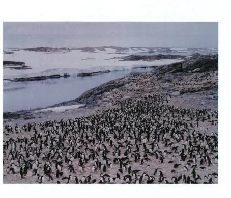
Adelie penguins are confined to areas where glaciers have formed moraines near the coasts, to provide nest-pebbles. Ainley (2002) argued that the availability of nest pebbles is a crucial driver of colony locations. In the Windmill Islands, most relic and extant colonies occur on raised-beach formations covered in rock debris measuring 2-6cm (Fig. 2.1). Keage (1982) argued that the preference for these formations demonstrates the importance of the availability of nest pebbles in determining colony locations. He wrote that the colony size and nest density are directly related to the availability of nest pebbles, with colony populations increasing with distance from the ice cap. However, he did not address the potential role played by penguins in building up these raised-beach formations by collecting nest-pebbles from surrounding areas.
Fig 2.1: Adelie penguin colony at Whitney Pt, January, 2006. This colony is undergoing a strong population increase (3900% more breeding pairs than when the colony was first counted in
1959/60).
Patterson, 1997).
Moczydlowski (1986; 1989) investigated the terrain properties of colony locations in the South Shetland Is. He found that the common features of all colonies were good drainage and high levels of solar radiation, with Adelie penguins nesting in the sites with the thinnest snow cover at the end of winter. In addition, their colonial nature helped shed snow because their faeces carried high levels of sodium chloride, which lowered the freezing point of water. This in turn aided dispersion of snow from colonies. From this, he concluded that Adelie penguins selected nest sites that are naturally likely to have the least amount of snow, and then, through the deposition of faeces, further increase the site's suitability. In 1986, Moczydlowski found that when penguins were not present, there was no difference in air temperature between colony sites and other parts of the landscape. He also argued that Adelie penguins did not nest in the most exposed sites. Instead, he proposed that they prefer sites with the least snow cover, but also with lower winds. Both Yeates and Moczydlowski's studies were conducted before the widespread availability of GIS as a tool for analysing spatial data. Their studies therefore did not take account of spatial variability within and among colonies.
At Cape Hallett, in the Ross Sea, Adelie penguins are found on well-drained mounds, and where these were flattened by human activities associated with the now-abandoned research station, Adelie penguins did not recolonise after the station closed. However, where those mounds remained or were rebuilt as part of habitat rehabilitation, the penguins reoccupied after the humans left (Wilson et al., 1990).
2.1.4 Climate variability and snow accumulation
conditions and other, finer-scale processes are likely to be involved.
A few studies have attempted to separate the effects of changes in sea-ice extent and snow accumulation patterns at local scales (Trivelpiece and Fraser, 1996; Fraser and Patterson, 1997; Patterson et al., 2003). On the Antarctic Peninsula, rising temperatures over the past 50 years have been accompanied by increasing snowfall and decreases in sea-ice extent — both factors which have been implicated in decreasing Adelie penguin breeding populations (Fraser and Patterson, 1997). Trivelpiece and Fraser (1996) studied population trends at Litchfield I, near Palmer Station on the Antarctic Peninsula. They noted that 18 of 21 colonies that have recently been abandoned were in the lee of prominent topographic features.
Patterson et al. (2003) used a GIS hillshade model as a proxy for snow accumulation on Litchfield I and nearby Torgersen I, in a bid to determine whether snow accumulation or the effects of human visitation could best explain the observed changes in colony population trends. The hillshade model could be seen more accurately as a surrogate for exposure to the prevailing winds. Their study found a strong correlation between wind exposure and population trends, and no statistically significant relationship between the rates of human visitation and population trends. One of the limitations of a hillshade model as a surrogate for snow accumulation is that it models light — which has a laminar flow, whereas wind flows turbulently, and the transport of snow is physically complex (e.g. Kind, 1986; Liston and Sturm, 1998; Green et al., 1999). Thus, a hillshade can only give a first approximation of the patterns of snow accumulation. Such an approximation is appropriate in sites with simple topography, but potentially less useful for fine scale studies in sites with more complex or finer-scale topographies, such as those around Casey, where the maximum altitude is about 35m above mean sea level, and the landscape is dominated by a mix of low cliffs and gently undulating plateaux.
2.1.5 Human impacts on Adelie penguins
variability from the effects of human activity at or near the colonies.
A number of studies have investigated the effect of human activities on Adelie penguins. Reasons given for this research include public concern that man's presence in Antarctica may damage the ecosystem (Wilson et al. 1991), the obligations of national research programs under the Antarctic Treaty and concerns that the effects of human activity may affect the results of scientific research (Clarke and Kerry, 1994; Wilson et al., 1989). National Antarctic science programs are obliged to minimise their effect on wildlife and the environment, under the Antarctic Treaty and the Madrid Protocol. The International Association of Antarctica Tour Operators (2006) stated that tourism operators are also obliged to meet the requirements of the Antarctic Treaty. Young (1990) noted that Adelie penguins and humans have very similar requirements in Antarctica, namely access to ice-free terrain near water, and that as human activities increase, so too do the chances of significant effects on Adelie penguins.
Adelie Penguins have often been considered to be relatively immune to human disturbances because they do not always display overt distress behaviours (Giese, 1996). However, numerous studies have attempted to investigate the effects of human activities on pygoscelid penguins. These activities include the destruction of penguin colonies (Micol and Jouventin, 2001); other alterations to the terrain from station construction (Wilson et al., 1990); aircraft flying over colonies (Culik et al., 1990; Wilson et al., 1991); manipulation of the birds during scientific studies (Wilson et al., 1990; Clark and Kerry, 1994, Giese, 1996) and pedestrian visits to colonies (Culik et al., 1990; Wilson et al., 1991; Woehler et al., Giese, 1996; 1994; Fraser and Patterson, 1997; Holmes et al., 2006). Measures used to determine the effects on penguins include behavioural changes, physiological changes such as heart rate (Wilson et al., 1991), changes in feeding behaviour (Wilson et al., 1989); and changes in breeding success or colony population trends (Woehler et al., 1994; Giese, 1996; Fraser and Patterson, 1997; Patterson et al., 2003).
1989). The researchers in that study concluded that this represented a "psychological" effect on the birds.
There is also some direct evidence of a long-term effect on Adelie penguin numbers as a result of human visits. Giese (1996) studied the effects of scientific nest checks conducted every second day and tourist-style visits two to four times every day in Adelie penguin colonies that had previously been exposed to little human activity. She found that colonies subjected to both treatments had lower breeding success than control colonies. This difference was significant in small colonies (-40 pairs) and not significant for larger colonies (-70 pairs). Giese argued that the effect of disturbance was exacerbated in smaller colonies and that it was most closely linked to the frequency of disturbance rather than the intensity of the disturbance.
Woehler et al., (1994) proposed that visits to colonies by station personnel were responsible for observed decreases in breeding success and populations of colonies at the end of Shirley I nearest Casey. An examination of Adelie penguin population trends on two islands near Palmer Station on the Antarctic Peninsula was unable to find a link between population trends and human activities (Fraser and Patterson, 1997). In that study, the most heavily visited island, Torgersen I, was also the one with the smallest decrease in Adelie penguin numbers. Young (1990) found that Adelie penguin numbers in colonies close to the research station at Cape Bird declined significantly, while the overall number of penguins in the breeding locality increased. Those colonies closest to the station were the ones that had been most intensively studied and were also within 200m of a helicopter landing pad.
At Cape Hallett, in the Ross Sea, Adelie penguins are known to nest on well-drained mounds (Wilson et al., 1990). The total population decreased from 62 900 pairs to 37 000 between 1959 and
Micol and Jouventin (2001) investigated the effects of station activities and the construction of a runway on the populations of 7 seabird species nesting near Dumont d'Urville, Antarctica. They found that despite the destruction of 10% of the region's Adelie penguin nests, the total number of Adelies had increased by 50% during the study period. On Ile des Petrels, where the station buildings are located and helicopters operate each summer, the number of Adelie penguins increased by 250%. Micol and Jouventin noted that they could not quantify the effect of environmental factors such as sea-ice extent, food availability and nest-site availability. However, they suggested that in the long term, these factors outweighed the apparently significant short-term effects of human construction activities.
It is unclear why the penguin populations of Cape Hallett and Dumont d'Urville should display such different responses to station activities. It may be that other environmental factors have confounded the results of one or both of these studies. Little of the literature has involved examination of variation among colonies within one breeding locality, which is the scale at which such impacts are most likely to be seen.
2.2 GIS habitat modelling
Geographic Information System analysis has rarely been used to examine the spatial ecology of Adelie penguins (Patterson et al., 2003). However, GIS has been widely used to investigate relationships between the landscape and numerous other species across the world (e.g. Aspinall and Veitch, 1993; Baker et al., 1995; Bian and West, 1997; Store and Kangas, 2001). GIS has enabled ecological studies to quantitatively analyse spatial variability (Burrough and McDonnell, 2000; Vogiatzakis, 2003). Store and Kangas (2001) also noted that GIS applications can generate new data by spatial analysis of existing data. Typically, GIS-based habitat analyses have involved the creation of spatial data layers, each of which represents one habitat parameter. These layers have then been combined, using some function — derived from either expert knowledge or statistical testing - to produce a map showing the relative quality of habitat for the species being examined (Store and Kangas, 2001).
conservation priorities (Bian and West, 1997; Walker and Craighead, 1997), field work and management planning (Curnutt et al., 2000), distribution and abundance modelling (Aspinall and Veitch, 1993); environmental impact assessments, as a step in refining habitat maps (Breininger et al., 1991), and to model changes in habitat suitability and fragmentation through time (Hansen et al., 2001).
Habitat prediction models have been found to produce stronger results for species that are common, range-restricted or more specialised than for species that are rare, wide-ranging and/or more generalised in their habitat requirements (Pereira and Itami, 1991; Debinski et al:, 1999). Adelie penguins can be considered to be common within breeding localities, though their specific habitat requirements are poorly understood (Yeates, 1975; Moczydlowski, 1986, 1989
Numerous approaches have been used to drive GIS-based habitat models, and one common classification method has been to split such models according to whether they are informed by field data (empirical models) and or by expert knowledge (rule-based models) (Guisan and Zimmermann, 2000; Store and Kangas, 2001). Store and Kangas (2001) argued that rule-based models were most suitable for situations in which it would be too expensive or time consuming to gather empirical data.
Rule-based models have been used for species for which good expert knowledge of habitat requirements was available, and the distribution poorly understood (e.g. Lauver et al., 2002). This approach has been considered suitable for those cryptic species whose presence/absence is difficult to map (Gibson et al., 2004). Rule-based models have often used similar techniques to multi-criteria decision making analysis (Pereira and Duckstein, 1993; Lenton et al., 2000), which is a common technique in GIS. In models using this approach, habitat parameters have typically been assigned values based on expert knowledge, and these factors then combined to produce habitat suitability maps (Breininger et al., 1991; Pereira and Duckstein, 1993; Curnutt et al., 2000; Hansen et al., 2001; Store and Kangas, 2001). Areas of suitable habitat have been defined as those areas in which all habitat factors coincide (Kelly et al., 2001). One criticism of this approach is that validation of these models has also often relied on expert knowledge, making the entire process somewhat circular (Pereira and Itami, 1991). •
parameters. The classification of habitat parameters has generally been independent of the wildlife data (Aspinall and Veitch, 1993). Adelie penguins are suited to empirical modelling because the penguins' present and past distribution is relatively easy to measure. In contrast, there is little expert knowledge available appropriate for forming rules to determine the location of colonies, as such processes are poorly understood (Yeats, 1975; Moczydlowski, 1986 and 1989; Wilson et al., 1990). The conspicuousness of Adelie penguin nests is in contrast to the problems encountered by researchers investigating bird species whose nest sites are cryptic and whose total populations and distributions must be inferred (Guisan and Zimmermann, 2000; Gibson et al., 2004).
Store and Kangas (2001) argued that the accuracy of the results of habitat analysis depends on the quality of the source data and of the analytical techniques. The most important factors affecting the quality of spatial data have been described as currency, completeness, consistency, accessibility, accuracy and precision, as well as the error sources inherent in the data-gathering processes. Error propagation also occurs through the analysis process, particularly as a result of combining data sets with different spatial and temporal scales (Burrough and McDonnell, 2000; Store and Kangas, 2001).
Input data for GIS habitat analyses have typically been derived from three main sources — remotely sensed photographs and images (Breininger et al., 1991; Aspinall and Veitch, 1993; Bian and West, 1997; Hansen et al., 2001; Osborne et al., 2001; Gibson et al., 2004); paper maps (Raphael et al., 1995; Lenton et al., 2000); and DEM derivatives (Raphael et al., 1995; Blackard and Dean, 1999; Guisan and Zimmermann, 2000; Gibson et al., 2004). Input data of animal or plant distribution have been gathered by survey (Aspinall and Veitch, 1993; Osborne et al., 2001; Gibson et al., 2004); or by radio or satellite tracking (Bian and West, 1997).
2004). Guisan and Zimmermann (2000) proposed that DEMs and their basic derivatives — slope, aspect and curvature — are generally the most accurate maps available, though they may not have the highest predictive potential. DEM derivatives may not have direct physiological relevance for a species, but can act indirectly on causative variables, such as temperature (Gibson et al., 2004). However, Vogiatzakis argued that these surrogate parameters may introduce errors into models. One result of using DEM-derivatives in a model is that the model may not be readily applied to other geographic areas because the same topographic position in a different region may experience a different environmental gradient (Guisan and Zimmermann, 2000; Austin, 2002; Gibson et al., 2004). However, Guisan and Zimmermann (2000) showed that at local scales, DEM derivatives may show strong correlations with species distributions.
Few GIS habitat analyses have accounted for temporal variability in habitat suitability (Curnutt et al., 2000). Guisan and Zimmermann (2000) noted that historical conditions may have a significant influence on the current distribution of organisms, and that most static models have failed to account for this. They urged researchers to incorporate historical data wherever possible. Guisan and.Zimmermann also noted that since temporal data of species' responses to environmental change are rarely available, static models are often the only possible approach. Cumutt et al. (2000) developed a model to account for changing hydrological conditions between years and between management scenarios. Baker et al. (1993) noted that selection of nest sites by sandhill cranes may have occurred when vegetation, climate patterns, water management or disturbance levels were different and that the suitability of an individual nest-site may vary from year to year. However, other studies that examined changing distributions of species have not considered temporal changes in the habitat quality (e.g. Glenz et al., 2001).
calibrating habitat suitability models has been the fact that any species rarely occupies all of its potential range (Curnutt et al., 2000). Fielding and Bell (1997) noted that prediction errors can occur in habitat models when the habitat is unsaturated. They warned that if the species under examination is not using the entire available habitat, this will generate interference in the model. It has also been argued that it often cannot be determined whether an animal has never, or will never use a particular location (Breininger et al., 1991). However, Curnutt et al. (2000) argued that while the species in question may not appear in all areas with suitable habitat indices, it should not appear in sites deemed to be unsuitable. Fielding and Bell (1997) suggested that such "false negatives" are likely to be the result of errors in either the statistical model or due to some relevant ecological process not being mapped. They warned that appropriate data may not be available for some ecological processes. Guisan and Zimmermann (2000) argued that nature is too complex and heterogeneous to be reduced a single predictive model, no matter how complex that model may be. Breininger et al. (1991) argued that long-term studies of population dynamics are needed to accurately quantify habitat suitability, but noted that this is beyond the scope of many mapping applications.
Scale
requirements at river basin and site-specific scales. Osborne et al. (2001) used datasets that had been acquired at different spatial scales before combining them into a single predictive model. Most GIS-based studies have worked at broad scales, with resolutions typically larger than lha (e.g. Manel et al., 1999; Glenz et al., 2001; Osborne et al., 2001; Gibson et al., 2004). Exceptions to this include Sieg and Becker (1990), who measured landscape variables within an 11.3m radius of• merlin (Falco columbarius) nests. If the ability to detect important landscape variables decreases as the resolution increases, as argued by Baker et al. (1995) it seems likely there's a need for more studies that use GIS-techniques to examine spatial variability at fine scales.
2.3 Statistics in GIS-based habitat modelling
A wide variety of multivariate statistical tests have been applied to GIS-based habitat modelling. The simplest models have operated entirely within a GIS, combining the data layers by some mathematical function (Guisan and Zimmermann, 2000; Store and Kangas, 2001). However, Guisan and Zimmermann (2000) warned that these tests have typically been inadequate for model-building as they did not allow stepwise selection procedures or graphical tests of model-fitting. More complex models have made use of the more powerful statistical tools available only in specialised statistical packages (e.g. Blackard and Dean, 1999; Debinski et al., 1999; Manel et al., 1999; Osborne et al., 2001; Gibson et al., 2004).
2.3.1 Univariate testing
The first step of statistical modelling of habitat suitability has often involved univariate exploration of the relationship between the dependent variable and each parameter (Manel et al., 1999). It has been argued that if a species selects habitat based on the measured parameters, those parameters should show differences in the mean and variance between sites, where the species is present and absent. Larger variation in the distribution of values has typically been expected in sites where the species is absent (Pereira and Itami, 1991).
2.3.2 Multivariate model selection
Multivariate analyses that have been widely used in GIS-based habitat suitability studies include discriminant analysis (Raphael et al., 1995; Manel et al., 1999; Debinski et al., 1999; Kidd and Ritchie, 2000); logistic regression (Sieg and Becker, 1990; Osborne et al., 2001); decision trees (Hansen et al., 2001), artificial neural networks (Blackard and Dean, 1999; Manel et al., 1999); generalised linear models (Gibson et al., 2004); and Bayesian approaches (Aspinall and Veitch, 1993).
One of the challenges in selecting an appropriate testing method is that few studies have compared the performance of different models. Exceptions to this include Blackard and Dean (1999) who compared the performance of two forms of discriminant analysis and artificial neural networks; and Manel et al. (1999) who compared discriminant analysis, artificial neural networks and logistic regression, in predicting the distribution of several Himalayan river bird species. Blackard and Dean found that an artificial neural network was significantly more powerful than either of the discriminant analysis functions, but found no significant difference in the results of the linear- and non-parametric discriminant analyses. They also noted that the artificial neural network took 2500 hours of computer run time, compared with five minutes for the discriminant analysis. Manel et al. (1999) found that the three methods they compared all had strong predictive power. When tested against calibration data, the artificial neural network outperformed the other two models, and discriminant analysis performed slightly better than logistic regression. When tested against datasets from different geographic areas, logistic regression marginally, but significantly outperformed the other two models, with the artificial neural network the worst-performer. They also found that the results from logistic regressions were most variable across species.
Discriminant analysis has been successfully used in ornithological studies to distinguish suitable habitat and the effect of human visitors on breeding populations (Debinski et al., 1999; Manel et al.,
1999; Patterson et al., 2003). However, it is limited in its applicability because of the underlying assumptions of normality, equal variance within each group and equal covariance matrices within each group (Flury and Riedwyl, 1988; Hastie et al., 2001).
Manel et al. (1999) noted that multivariate normality can be hard to assess, especially with large numbers of predictor variables. They argued that as normal distributions are an underlying assumption of discriminant analysis, the results should always be treated with caution. However, Blackard and Dean (1999) argued that in practice, the assumptions of discriminant analysis are often violated with minimal apparent effect on the result.
Logistic regression has also been widely used in ecological models (Sieg and Becker, 1990; Pereira and Itami, 1991; Bian and West, 1997; Glenz et al., 1999; Kelly et al., 2001; Osborne et al., 2001). This approach has been considered the most suitable when some of the available data were qualitative and did not meet assumptions of multivariate normality (e.g. Pereira and Itami, 1991). • Hansen et al. (2001) used a hybrid decision tree to classify habitat units. They wrote that this approach allowed them to incorporate different data types in the data analysis. Decision trees are non-parametric and hence make no assumptions about the distribution of the data (Quinn and Keough, 2002). Because decision trees attempt to predict each data point exactly, they avoid the need to characterise the model fit (Guisan and Zimmermann, 2000). Such trees have been found to generate almost as many terminal nodes as there are observations, and to therefore not offer any modelling parsimony. Pruning and cross-validation have typically been used to find an "optimal" balance between the number of terminal nodes and the predictive power (Guisan and Zimmermann, 2000).
2.3.3 Model refinement
2.3.4 Testing validity
The most common method for assessing the performance of a statistical model has been to report the overall percentage of correct predictions (Sieg and Becker, 1990; Raphael et al., 1995; Debinski
•
et al., 1999). Some researchers have tested model performance by cross-validation (Sieg and Becker, 1990). However, it has been argued that cross-validation provides an overly optimistic assessment of the predictive power of the model (Fielding and Bell, 1997; Guisan and Zimmermann, 2000).
Blackard and Dean (1999) and Guisan and Zimmermann (2000) argued that the optimal method for validating a model is to test it on independently collected data. This approach has only been possible in situations where independent datasets were available (Lauver et al., 2002). Guisan and Zimmermann suggested that where a single, large dataset is available, splitting that set into training and testing groups is appropriate. This approach was taken by Blackard and Dean (1999) and Manel et al. (2000). Fielding and Bell suggested that splitting a dataset into training and test sets can cause problems if the original data set is small. This has been a particular problem for studies of rare or cryptic species, with few positive records (e.g. Gibson et al., 2004).
2.4
Snow accumulation modelling
2.4.1 Snow transport mechanisms
Snow drift is an important element in mass-balancing processes in polar and alpine environments because of its potential to move large volumes of snow during strong surface wind events (Kind, 1986; Greene et al., 1999; Bintanja et al., 2001; Doorschot et al., 2004). Snow enters the environment as precipitation, which is not distributed uniformly across the landscape when it occurs in windy conditions (Kind, 1986). Precipitation tends to accumulate on leeward slopes, but this process is poorly understood and rarely incorporated in models of snow accumulation (Lehning et al., 2000).
may be almost snow-free, while gentle slopes may show a uniform snow distribution (Jaedicke et al., 2000). Deep snowdrifts occur where the areas of ablation are larger than the areas of accumulation (Liston and Sturm, 1998). It has been argued that topography is a crucial driver of snow accumulation patterns because changes in wind direction are more important than changes in wind speed in determining snow deposition (Liston and Sturm, 1998). It has also been found that the heaviest snow drift events occur during periods of roughly constant strong winds, and that short but strong blasts do not produce significant snow drift (Michaux et al., 2002).
The dominant snow transport methods are saltation and turbulent suspension (Kind, 1986; Liston and Sturm, 1998). Creep (the gradual down-slope movement of crystals) also shifts snow, but it is rarely incorporated in flux modelling because of its very small contribution to total flux (Uematsu et al., 1991; Jaedicke et al., 2000). Saltation is the motion of snow crystals bouncing in a flow-layer several centimetres above the snow layer (Kind, 1976; Kind, 1986; Pomeroy et al., 1997; Lehning et al., 2000; Whittow, 2000). Saltation occurs when the wind produces a shear stress that exceeds the amount of stress needed to shatter the bonds of snow surface crystals. It is considered to be responsible for up to 25% of annual snow transport; with the proportion dropping as wind speed increases (Pomeroy et al., 1997; Haehnel et al. 2001). Once snow is moving by saltation, it is available to become suspended in the zone of turbulent flow (Kind, 1976; Kind, 1986; Pomeroy et al., 1997; Lehning et al., 2000). The term turbulent flow describes the net forward movement of air in an irregular, eddying flow, and it stretches tens of metres above the snow surface (Whittow, 2000; Pomeroy et al., 1997).
In addition to snow being redistributed, a significant amount is lost through sublimation. This is the conversion of ice crystals to vapour (Pomeroy et al., 1997). In one study in the Arctic, sublimation losses were calculated at 9-22% of the winter precipitation, with sublimation accounting for up to half the winter precipitation falling on windward slopes (Liston and Sturm, 1998).
2.4.2 Why snow accumulation is modelled
2001), ecological studies (Evans et al., 1989, Greene et al., 1999; Ishigawa and Sawagaki, 2001) and management of recreational sites such as rock climbing areas and ski runs (Purves et al., 1998).
2.4.3 Available snow accumulation models
Snow accumulation models vary in both complexity and accuracy, depending on the available input data and required results: Most of the early models operated in two dimensions (Greene et al.,
1999), and were designed to predict the evolution of snowdrifts and the distribution of snow along the line of the prevailing wind direction (Liston and Sturm, 1998). Attempts to take into account the three-dimensional spatial variability of snow accumulation patterns are more recent (Daly et al., 2000). One method of classifying models is into those that attempt to provide numerical snow depths (e.g. Pomeroy et al., 1997; Greene et al., 1999; Lehning et al., 2000); and those that provide a relative map of snow distribution (e.g. Purves et al., 1998; Ishigawa and Sawagaki, 2001).
Attempts to model snow accumulation are complicated by the challenges involved in measuring precipitation and snow flux. These challenges include disturbing influences such as low temperatures, high humidity, riming and the difficulty of distinguishing fresh precipitation from drifting snow (Doorschot et al., 2004). Attempts to measure snow flux have used pulse-counting sensors, mechanical traps, acoustic and optic sensors (Bintanja et al., 2001; Doorschot et al., 2004). These measurement difficulties are reflected in the fact that the Australian Bureau of Meteorology does not record precipitation at its Antarctic weather stations (AADC, 2006).
A criticism of many snow accumulation models, such as those described in Pomeroy et al. (1997) and Lehning et al. (2000) has been that they are too complicated for easy assimilation into models such as those used for hydrological management (Walter et al., 2004). There have been attempts in recent years to develop relatively simple snow-distribution models, because of concern that the earlier, mechanistic models were overly complex (Walter et al., 2004). These simpler models typically set a constant value for variables such as snow density and threshold shear velocity, despite the spatial variability of these values (Liston and Sturm, 1998).
parameters (typically Solar radiation, wind speed, air temperature, humidity and precipitation) are likely to vary significantly (Daly et al., 2000).
In addition to the meteorological inputs, models typically require an initial snow cover layer. Researchers have used a variety of methods to assess the initial snow cover. These include using radar to measure snow depth (Jaedicke et al., 2000) and manually measuring snow depths along transects (Evans et al., 1989). Such approaches are inappropriate for modelling historic snow cover, or for modelling snow cover in areas that are not readily accessible.
Some of the most prominent snow accumulation models are briefly described here. The Prairie Blowing Snow Model (Pomeroy et al., 1993) was physically based and was found to predict snow accumulation to within 10% of observed snow depths. However, its complexity and data requirements meant that its use was restricted to areas with major climatological stations, and is hence unsuitable for polar environments (Pomeroy et al., 1997). The Distributed Blowing Snow Model was developed for Arctic conditions from the Prairie Blowing Snow Model. This model divided the terrain into homogeneous landscape elements, based on vegetation, terrain, exposure and fetch characteristics. Meteorological observations were used to model the snow transportation processes (Pomeroy et al., 1997). Such an approach ignores the continuous nature of landscape variables, and is considered to be not suitable for adaptation to fine-scale applications such as this study.
Another model, SnowPack (Lehning et al., 2000; Doorschot et al., 2004) was designed for avalanche prediction. Its focus is on modelling the stability of the snow-pack and it therefore required input data related to crystal structure of the snow pack. The model was designed for steep alpine environments, and required input from a network of about 100 weather stations in the Swiss Alps (Lehning et al., 2004). In steep terrain, there is also the potential to use remotely triggered cameras to measure changes in snow distribution, which can then be used as inputs for the development of a statistical model (e.g. Tappeiner et al., 2001).
The SnowTran-3D model (Liston and Sturm, 1998; Greene et al., 1999) attempted to model three-dimensional snow movement for treeless terrain in the Alaskan Arctic. It was designed to help with water resource management and has been adapted for integration with a GIS (Haehnel et al., 2001). This model accounted for transport variations resulting from accelerating and decelerating flow, using solar radiation, precipitation, wind speed and direction, air temperature, humidity, topography and vegetation snow-holding capacity. It has been argued that SnowTran is only suitable for areas with gentle terrain (Lehning et al., 2000) because it assumes that the wind direction is not affected by the topography.
Scale
One of the principle constraints on snow accumulation modelling is its demand for computational power. Thus, attempts at snow modelling are typically limited in spatial and temporal scale scales (Hageli and McClung, 2000). Problems associated with scale are common with snow accumulation models. These include the inability of regular meteorological measurements to capture fine-scale processes such as snow drift; the inability of snow profile measurements to capture spatial variability and contradictions between input and output scales.
2.4.4 Commonly used physical inputs
Wind Flow Field •
Topography alters the speed and direction of the wind flow (Liston and Sturm, 1998; Lehning et al., 2000). Therefore, a robust wind field model has been considered to be an important part of many snow accumulation models (Purves et al., 1998; Liston and Sturm, 1998; Haehnel et al., 2001; Walter et al., 2005). Most of the available algorithms to measure this are based on the slope and aspect of cells. In contrast, Liston and Sturm (1998) elected not to model a wind field because their model was designed for relatively gentle terrain, and excluding a wind field model reduced computational expense.
Wind Shear Stress
The wind speed required to shift snow is dependent on factors such as the age and density of the snow and the temperature and humidity of the air (Doorschot et al., 2004). However, some snowdrift models have used a constant value for this threshold (Purves et al., 1998; Greene et al., 1999). Once the wind shear stress exceeds the threshold, snow begins to move. Modelled wind shear velocity has generally been calculated from the wind flow field and the surface roughness (Liston and Sturm, 1998; Haehnel et al., 2001) and may also take into account the air and snow density (Jaedicke et al., 2000). Liston and Sturm (1998) argued that the threshold changes very slowly in low temperatures, and that a constant value is suitable for environments such as the winter Arctic. They found that attempts to introduce more complex and realistic shear thresholds did not
•improve the results of their model.
A few models have included no measure of wind shear (Tappeiner et al., 2001; Purves et al., 1998; Orndorff and Van Hoesen, 2001). Tappeiner et al (2001) and Orndorff and Van Hoesen (2001) attempted to explain snow accumulation based on terrain characteristics rather than on weather inputs.
Saltation and Suspension
Sturm (1998) has been followed by others (e.g. Haehnel et al., 2001; Walter et al., 2004; Parajka et al., 2005).
The availability of snow for drifting is largely density dependent. Some models operated on the assumption that old snow is too dense to be easily transported, and that only fresh snow is available for transport (Walter et al., 2004). Purves et al. (1998) argued that during melting periods, no drift would occur, apart from that of precipitating snow. They argued that if a melt-freeze cycle occurs without snow falling during the freeze period; it could be assumed the shear velocity would be so high as to prevent any erosion.
Sublimation
Sublimation is the evaporation of snow to water vapour (Whittow, 2000). The relative importance of sublimation in snow dynamics is driven by factors such as temperature and wind speed, with the sublimation rate increasing as temperatures and wind speeds rise (Pomeroy et al., 1997; Liston and Sturm, 1998). Sublimation calculations require information on the size of the snow crystals (Pomeroy et al., 1993).
Precipitation
Precipitation was a key input for most snow accumulation models (Purves et al., 1998; Lehning et al., 1999; Daly et al., 2000; Orndorff and Van 'Hoesen, 2001; Tappeiner etal., 2001). However, in polar environments, precipitation may be a less important source of snow than accumulation by horizontal transport (Liston and Sturm, 1998; Seppelt and Connell, 2005).
Initial snow layer
3 Chapter 3: Data and Methods
3.1 3.1 Study areas
3.1.1 Windmill Is
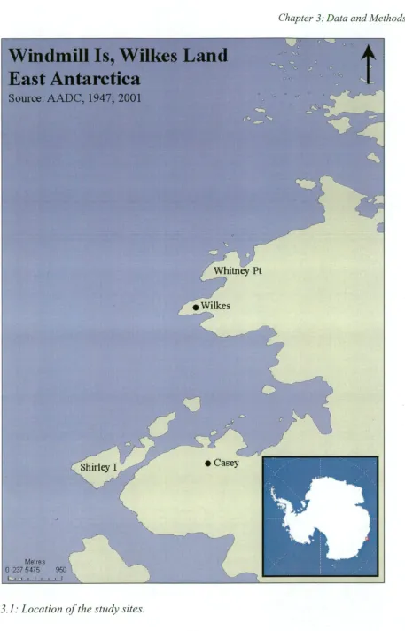
The Windmill Is are the islands and coastline covering an area of about 75-801= 2 around Casey (66°17'S, 110°32'E) Wilkes Land, East Antarctica (Fig. 3.1). They comprise four large peninsulas and more than 30 islands (Murray and Luders, 1990; Kirkup et al., 2002). During summer, the Windmill Is contain the only extensive areas of snow-free land for about 800km of coast around Casey (Murray and Luders, 1990; Kent et al., 1998).
The Windmill Is contain extant penguin colonies on fourteen islands and peninsulas. The region's total population was estimated at 93 092 ±9300 pairs in 1990 (Woehler et al., 1991). Historically, colonies have also existed in other parts of the region, such as the Bailey Peninsula (Emslie and Woehler, 2005). Colonies have been monitored on Shirley I, Whitney Pt, Blakeney Pt, the Frazier Is, Odbert I, Ardery I and Peterson I during the period of human habitation.
3.1.2 Geology
Windmill Is, Wilkes Land
East Antarctica
Source: AADC, 1947; 2001
Whitney Pt
[image:48.562.51.508.41.753.2]Metres 0 2375475 950
3.1.3 Weather
The weather around Casey is frigid-Antarctic (Melick et al., 1994). Weather observations between 1989 and 2004 showed that in the warmest month, January, the mean daily maximum temperature was 2.1°C and the mean minimum was -2.6°C. October was the coldest month of the breeding season and also the time when Adelie penguins arrived at the colonies. During October, the mean daily temperature range was -15.3°C to -8.3°C. The area had a modelled mean annual snowfall of 224.6mm (snow water equivalent) (Bureau of Meteorology, 2004). Between 1996 and 2006, monthly mean wind directions ranged between 92.3° and 186.1°, with the prevailing winds coming from ESE. During the Adelie penguin breeding seasons in this decade, the mean wind speed was 12.64 knots, with a mean monthly maximum wind gust of 65.06 knots. During that decade, breeding seasons had a mean 32.5 days in which winds exceeded gale force (37kts) (AADC, 2006).
3.1.4 Human history
Humans have visited and occupied the Windmill Is since the USA Navy's Operation Windmill in 1947-48. The USA established the Wilkes research station (66°15.4'S, 110°31.5'E) in 1957. The Wilkes base was handed over to the Australian government in 1960. The Australians inhabited Wilkes until 1969, when they shifted to the Casey Tunnel (66°16.7'S, 110°31.5E), which is located between the current Casey site (66°15.9'S, 110°31.8'E) and the coast. In 1989, the station was shifted to its current site (Woehler et al., 1991; Bureau of Meteorology, 2006). Personnel in both the Australian and American programs undertook scientific research at both Shirley I and Whitney Pt (e.g. Penney, 1968; Kent et al., 1998; Woehler et al., 1994). In 2005/06, Casey housed 53-60 personnel during summer, and 20 during winter.
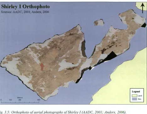
3.1.5 Shirley I