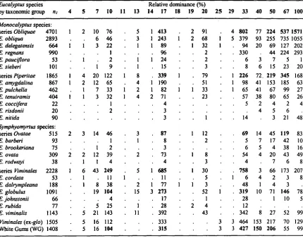
Predicting eucalypt distributions
in Tasmania
An application of generalised linear modelling
Volume Two
Kristen J. Williams B.Sc.(Hons)
Submitted in fulfilment of the requirements
for the degree of
Doctor of Philosophy
Volume Two of Two
Probability
of
occurring
Environmental gradient
7.1 Introduction
The previous experimental chapters have been stages in the development of an empirical analysis of Eucalyptus species' distributions in Tasmania. In order to predict species' distributions from
an ad hoc set of compiled ecological data, important statistical and ecological assumptions of the
data and its analysis were considered; these were: (i) the sampling adequacy of eucalypt forest habitat (Chapter 2); (ii) the sampling domains for individual species' occurrences and their representativeness (Chapter 3); and the suitability of deriving (iii) resource (Chapters 4 & 5) and (iv) productivity gradients (Chapter 6) as predictors of plant distribution patterns. The current chapter applies the fmdings of previous chapters to the development of a realised niche model for
Eucalyptus globulus subsp. globulus (hereafter expressed as E. globulus) in Tasmania. In doing
so, aspects of the ecology of this species are considered in the context of its physiological tolerance, competition, predation, disturbance and historical processes.
Eucalyptus globulus is a Symphyomyrtus species of open forests and woodlands in southeastern
Australia. Its natural range forms part of the native forest wood resource, and its rapid growth and good wood properties have lead to intensive research into its selective breeding and plantation silviculture (e.g. Borralho & Potts 1996; Bennett et al. 1997). Eucalyptus globulus
occurs throughout coastal regions of eastern Tasmania (Williams & Potts 1996, p. 69) where its spring and summer flowering are also important to the breeding success of swift parrots, a threatened species in Australia (Brereton 1997). In these regions it is widespread as a minor species in wet and dry sclerophyll forest stands that are usually dominated by species from the subgenus Monocalyptus (e.g. Duncan & Brown 1985; Kirkpatrick etal. 1988a). Few populations
extend far inland from the coast where there are larger seasonal and diurnal temperature ranges, and winter frosts are common (Kirkpatrick 1975a, b). Several highly disjunct populations are also known from western and southwestern coastal areas, and occurrences on King Island are believed to be remnants of their former extent (e.g. Wells 1989). Eucalyptus globulus also occurs
on mainland Australia where it is generally restricted to southern coastal Victoria around Cape Otway, the Strzelecici Ranges and Wilsons Promontory (e.g. Kirkpatrick 1975a, b; Jordan et al.
1993). However, as the current set of ecological data does not include representative sampling for forest habitats in western regions and King Island, only the populations in eastern regions of Tasmania (Finders Island to Recherche Bay) were considered in this analysis of its realised niche.
Despite little variation in key taxonomic traits (e.g. capsule morphology, Jordan et al. 1993), Eucalyptus globulus is not a genetically homogenous species in Tasmania. The accumulated
Chapter Seven: Modelling the Realised Niche
1994a, b; Nesbitt et al. 1995a, b; Jackson 1997; Kelly 1997) indicates considerable genetic
differentiation of northern and southern populations (e.g. Dutkowski 1995; Dutkowski & Potts in prep.; Dutkowslci etal. 1997). The most recent classification distinguishes five major
genetically-differentiated geographical races in eastern Tasmania (Dutkowski et a/. 1997), these are from
north to south: Furneaux Group, Northeastern Tasmania, Southeastern Tasmania, Southern Tasmania and Recherche Bay. A minor southern race (Dromedary) in the Derwent Valley is also recognised.
In Tasmania, E. globulus often dominates grassy dry forest communities in lowland, coastal
regions of the southeast and heathy woodland on Flinders Island (Duncan & Brown 1985). In these situations E. globulus frequently co-occurs with the wide-spread Symphyomyrtus species E. viminalis, and the two species vary in their patterns of relative dominance. However, the most
widespread occurrences of E. globulus are as a minor species in wet and dry sclerophyll forests
(e.g. Kirkpatrick et al. 1988a; Duncan & Brown 1985), but E. globulus then occurs singly or in
pure stands in specific habitats within these forests (e.g. Hogg & Kirkpatrick 1974; Kirkpatrick & Nunez 1980; Kirkpatrick & Marks 1985; Kirkpatrick 1986). Such widespread coexistence between species from different Eucalyptus subgenera, especially in southeastern Australia, has
become known as Pryor's rule (after Pryor 1953, 1959a, b; e.g. Sinclair 1980; Florence 1981, 1996; Kirkpatrick 1981; Austin et a/.1983b, 1996; Noble 1989).
In Tasmania, the Eucalyptus subgenera are represented only by Monocalyptus and
Symphyomyrtus species, reflecting quite different phylogenetic lineages (Ladiges et al. 1995;
Ladiges 1997). Species from either subgenera are reproductively isolated (Ellis etal. 1991), and
with unequivocal differences in physiological traits of leaf chemistry, root system processes, and establishment and regeneration niche processes, their coexistence (and Pryor's rule) may be explained in terms of complementary niche requirements (Noble 1989; see also Florence 1996). The specific ecological role of E. globulus as a Symphyomyrtus species that frequently coexists
with other Eucalyptus species from the subgenus Monocalyptus is poorly understood. However,
it is unlikely that the patterns of co-occurrence represent a simple accident of similar physiological responses or the random outcome of competitive interactions. Rather, mixed-species stands may reflect mechanisms of ecological feedback that promote the retention of forest on a site in the presence of a fluctuating and sometimes harsh environment.
Competitive interactions between species from different subgenera are likely to be diffuse, the outcome of relationships having been largely decided during the 'transient niches' (sensu Noble
1989) of seedling establishment and forest regeneration (e.g. Duff et al. 1983; Stoneman 1994;
Ashton & Martin 1996; Florence 1996). However, co-occurrences between E. globulus and a
phyogenetically related species, such as E. viminalis (both from the series Viminales), are also
quite frequent (e.g. Duncan & Brown 1985). Coexistence between species within subgenera, that are potentially inter-breeding (e.g. Griffin et a/. 1988) and exhibit similar strategies of
patterns of association between E. globulus and E. viminalis are likely to reflect more direct mechanisms of competition. As E. viminalis is a clinal species with E. dalrympleana and E. rubida (e.g. Phillips & Reid 1980), then competitive interactions with E. globulus may also extend to these species. Therefore, the possibility that competitive interactions between
E. globulus and the clinal white gum species may have influenced the extant distributions of either species, is considered in the context of their patterns of co-occurrence and dominance
within the distributional range of E. globulus in eastern regions of Tasmania.
Occurrences of E. globulus in eastern regions of Tasmania also straddle two divergent forest types that are typically dominated by Monocalyptus species from different series. The wet sclerophyll forests are usually dominated by an ash species (e.g. E. obhqua; series Obliquae) (Kirkpatrick etal. 1988a) and the dry sclerophyll forests are most typically dominated by a peppermint species (e.g. E. amygdalina, E. pukhella, E. tenuiramis; series Piperitae) (Duncan & Brown 1985). Continuous ecotonal variation exists between these stand types dominated by
species from either series, and some complex combinations exist. However, quite different
ecological processes are associated with either forest type, requiring different strategies of
regeneration (Florence 1996).
At one extreme, the closed-canopy, wet sclerophyll forests of relatively tall, even-aged trees are
typically subject to infrequent, high intensity and large scale disturbance due to wildfire (e.g.
Gilbert 1959; Luke & McArthur 1978). Adult trees are often killed and forest recovery is largely
through episodic seedling regeneration on an ash-bed, with rapid growth rates and intense
competition for light (e.g. Cremer & Mount 1965; Attiwill 1994; Chambers & Attiwill 1994;
Ashton & Kelliher 1996).
At the other extreme, dry sclerophyll forest can be typified by a multi-aged and multi-layered
canopy, the result of many cycles of variable-scale patch disturbance due to variable intensity
fires and the frequent recurrence of drought (e.g. Withers & Ashton 1977; Duncan 1981;
Williams etal. 1994). Regeneration strategies are equally diverse and may involve coppice recovery from stem or lignotuber buds, or seedling regeneration in larger canopy gaps with the
long-term persistence of lignotuberous seedlings before suppressive or drought conditions are
released (e.g. Noble 1984; Possingham etal. 1995; Strasser etal. 1996; Facelli & Ladd 1996).
Therefore the widespread distribution of E. globulus across both wet and dry forests would suggest a generalised ecological response, or genetically divergent ecotypes.
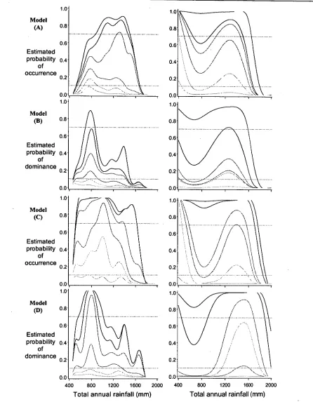
The present chapter largely relies on climatic indices to model the realised niche of E. globulus within its sampling domain corresponding to the eastern regions of Tasmania. Univariate
responses and patterns of occurrence or dominance in wet and dry forests, or with other
eucalypts, are initially examined. These exploratory analyses form a foundation for developing
Chapter Seven: Modelling the Realised Niche
1. What are the important environmental gradients delimiting the distribution of E. globulus and what form does the response of E. globulus take (e.g. simple or complex)?
2. Can biotic explanatory variables, such as forest stand structure (e.g. attributes for stand height and stand cover) and/or response functions for relative dominance be used with abiotic factors to better predict the distribution of E. globulus?
3. If the response shapes are complex, can these be simplified by separating the distribution of E. globulus into different ecological types (e.g. wet sclerophyll or dry sclerophyll forest occurrences)?
4. Can the distribution of E. globulus be clarified by taking into account competition with related species in the series Viminales?
5. Can the models, so developed, be interpreted in terms of known eco-physiological processes and limiting responses?
The ecological response shapes revealed by these models also enable some of the propositions based on the continuum concept (Austin & Smith 1989; Austin & Gaywood 1994) to be
explored. For instance, Austin & Smith (1989) suggested that because of interactions with other species, the shape of a species' realised niche could take complex forms. They indicated that mechanisms associated with the complexity of the ecological responses might include
competitive exploitation of the resource at low levels, light competition with canopy closure at intermediate levels; and at high resource levels, an interaction between competition for light and physiological tolerance of toxic conditions. Where greater partitioning of responses occurred along direct environmental gradients, this was expected to be due to differential physiological adaptations between species.
Theoretically, it may be expected that competition between coexisting species could arise if their physiological optima approximately coincide on one or more environmental gradients of their fundamental niche (Austin & Smith 1989). Interaction between such populations of related species would be expected to lead to a divergence in their ecological optima, since one species will generally have a performance advantage over the other. The species that is the more effective competitor would be expected to maintain its ecological optimum closer to it
physiological optimum (Austin & Smith 1989). Conversely if two species that co-occur do not compete, but instead partition the environment, then it may be expected that their ecological optima are randomly related to each other; that their ecological optima may or may not coincide. In such a case of neutral association, their ecological optima may have little relationship to the position of their physiological optimum, but may be related to other factors of their environment (e.g. competition due to another species, predation, disturbance, the distribution of historical environments). However, if the two species were in a mutually dependent or facultative association, then coincidence between their ecological optima would be expected. Again, this may or may not reflect a coincidence of their physiological optima.
Ecological
performance Pure stands
Mixed-species
stands Pure stands
E. viminalis E. globulus
Environmental gradient
species may occupy a site to the exclusion of the other because it is a more effective competitor of available resources, or it is more tolerant of environmental stress. Either species may vary in this respect by their response to different gradients in water, temperature, light and nutrient status. For example, E. globulus may be a more effective competitor for resources than
E. viminalis when environmental conditions are also associated with warm, equable temperatures and a high substrate nutrient status, dominating at both the mesic and dry end of a gradient. Conversely, on the cooler sites with more variable seasonal and diurnal temperature ranges,
E. viminalis may dominate over E. globulus on both mesic and drought-prone sites. While the two species may appear to coincide along a gradient in nutrient status, and to some extent water supply, they may clearly differentiate along gradients in temperature and its interaction with water.
Mixed species stands may therefore arise because intermediate conditions result in neither species having a distinct performance advantage over the other, relative to the position of their optimum responses (Fig. 7.1). Depending upon their respective position along a key
environmental gradient (e.g. temperature conditions), the symmetry of their competitive
interactions may also shift. Thus, their resulting patterns of co-occurrence in the landscape might be expected to consist of continuous variation in stand dominance among populations comprising both species — following a gradient in the respective symmetry of their competitive interactions and trade-offs in their physiological growth or stress responses.
Figure 7.1 Putative occurrence of pure and mixed-species stands of two closely related species (e.g. E. globulus and
E. viminalis) with respect to an environmental gradient. Mixed species stands exist where symmetric competition leads to stable coexistence since neither species has a complete advantage over the other. As the
environment approaches the optimum habitat for either species, mixed stands are
progressively dominated by the
favoured species, but pure stands are expected in optimum habitat.
In the context of the continuum concept, the outcome of such interactions could be observed as the ecological response from the patterns of presence or absence, or relative abundance, of each species across a range of sites with similar types of environment (Fig. 7.1). Although competition is not expected to be restricted to two dimensions (i.e. due to competitive hierarchies, e.g.
Chapter Seven: Modelling the Realised Niche
1. A competitive interaction (negative) between potentially coexisting species will result in ecological optima that are displaced relative to each other.
2. The most effective competitor will maintain an ecological optimum closer to its physiological optimum than is the case for the other species.
3. Two species that passively co-occur will have ecological optima that are randomly associated with each other (ecological optima may or may not coincide), and may or may not reflect a coincidence with physiological optima.
4. Two species that interact positively will have ecological optima that coincide or nearly coincide, and this also may or may not reflect a coincidence with physiological optima.
A gradient analysis of the distribution of E. globulus could therefore reveal some of the underlying ecological relationships associated with its patterns of occurrence in eastern
Tasmania.
7.2 Methods
7.2.1 Database for occurrences of Eucalyptus globulus
A sample of E. globulus habitats (c. 0.25 ha plots) were obtained from an ecological dataset that was compiled for the general purpose of modelling the distribution of Eucalyptus species in
Tasmania (see Chapters 2 and 3). The appropriate sampling domain for modelling the gradient responses of E. globulus was defined from its known geographic and altitude ranges (Chapter 3).
This sampling domain delineation was believed important because numerous absence values beyond the environmental limits of a species (termed 'naughty-noughts' by Austin 1979) were expected to distort response shapes in subsequent predictive modelling (Austin & Meyers 1996). This sample includes presence, absence, or relative dominance for E. globulus and associated Eucalyptus species. Climatic indices were defined by monthly estimates derived from the spatial
locations (latitude, longitude, altitude) through ESOCLIM (McMahon et al. 1996). A nutrient index
was broadly defined from a classification of parent rock types (after Nix et al. 1992). The majority of habitats in eastern regions of Tasmania are associated with a moderate to high
nutrient status derived from the sedimentary substrates of Permian to Quaternary age, or rocks of
igneous origin (Devonian granite, Jurassic dolerite and Tertiary basalt).
Forest type was readily classified from community attributes associated with these samples. A set
of rules separated the predominantly southern wet eucalypt or northern dry sclerophyll stands by
understorey floristics, canopy height and overstorey tree species by general reference to the
classifications of Duncan & Brown (1985) and Kirkpatrick etal. (1988a), and depending upon the site detail available with each record (see Chapter 3). However, continuous variation between
the floristic and structural composition of the forest stands was evident, and the classification into
types was sometimes arbitrary. A comparison between the eucalypt community variability in the ecological dataset and the published accounts indicated that the forest communities in which
E. globulus is present as the canopy dominant or codominant are adequately represented (Chapter
A previous analysis of the representation of eucalypt forest habitats (Chapter 2) indicated that
samples were reasonably well-represented for eastern regions of Tasmania, but that occurrences
at higher altitudes (i.e. > 600 to 900 m) and in Midland regions were limited. In particular,
despite the large number of samples, the extensive areas of lowland Permo-Triassic sediments in
the Southern Midlands were under-represented, as were samples on Quaternary deposits in the
Northeast region (see Table 2.13). Consistent with this analysis, the sample of E. globulus occurrences (presences and absences) were found to be reasonably representative of its known
geographic range in eastern Tasmania (see Tables 3.6 and 3.16). However, both analyses suggest
that the level of replication associated with these samples would result in predictions with a
resolution of no more than about a 1:100 000 to 1:500 000 mapping scale, assuming consistency
between sample data and mapping data. This represents a classification of ecological variability
at the scale of ecosection to ecodistrict, representing spatial units of 25 to 10 000 ha (Klijn & Udo de Haes 1994). These analyses thus define the limiting resolution for summarising the
realised niche of E. globulus from the current sample, and suggest that some degree of sampling bias associated with under-sampled highland and Midland regions could influence the outcome
and should be taken into account when interpreting mapped predictions and direct gradient
responses.
The sample data for modelling the realised niche of E. globulus therefore comprises 1092 presences that represent approximately two-thirds of its known geographic range, and with a
further 4154 absence records, this geographic representation increases to 81% (Chapter 3).
Taking into account the altitude ranges for E. globulus (generally well below 700 m), the number of absence records reduces to 3980 observations, excluding an unverified outlying presence (830
m near St Marys, northeast Tasmania — see Williams & Potts 1996, p. 70). While this sample
for E. globulus has been classified as reasonably representative of its broad geographic and altitude ranges, it is under-represented for lowland occurrences below 100 m (a.s.1.) (see Table
3.8). Within this sampling domain, occurrences of E. globulus are not specifically related to any particular substrate, although there are more sites than might be randomly expected on Devonian
granites and fewer sites than might be expected on the Mathinna beds (see Table 3.11).
7.2.2 Rank order dominance and the calculation of relative dominance
Canopy dominance
Forest stand dominance has been defined as the relative position of a tree within a canopy. For
example, Florence (1996) refers to the dominant tree or species within a forest stand as that with
the most emergent canopy. Such a species is in a pre-emptive position for intercepting light and
will shade the canopies of adjacent species of lesser height. If these adjacent species are also
shade-intolerant, their growth will be suppressed relative to the dominant. However, in many dry
sclerophyll forest stands, multi-layered, relatively open canopies are common (e.g. Duncan &
Chapter Seven: Modelling the Realised Niche
Ecological dominance
An alternative definition of stand dominance considers the relative abundance of coexisting species, as a general indication of their respective levels of resource use (above and below ground) within the defined area of a forest stand. For example, ecologists generally observe the relationship between forest species by recording both their structural positions within the forest stand (e.g. height and cover) and their relative dominance (e.g. Mackey 1993a, b). This enables species to be qualitatively distinguished, taking into account their different ecological traits and physiological responses that may differentially suit their occupation of the site in which they are found. A definition of stand dominance based on canopy position alone (sensu Florence 1996)
cannot attribute differences to the partitioning of resources between species, and the significance of this variability between sites. However, ecologists are not necessarily completely consistent in their qualitative observations of forest structural and compositional characteristics. Therefore, when these data are compiled, only a more generalised estimate of the overall importance of one species relative to another can be made.
7.2.2.1 Rank-order dominance
The sample of ecological data for eucalypt occurrences was derived from two main sources: floristic surveys (e.g. Duncan & Brown 1985) and forest inventory (e.g. Lawrence 1978). The former records species dominance in the sense of relative abundance (e.g. Braun-Blanquet scores, Mueller-Dombios & Ellenberg 1974), and the latter records stem diameters for individual trees (i.e. basal area). The compiled estimate of dominance by individual Eucalyptus species
therefore consists of the simple rank order of dominance exerted by an individual species, irrespective of the standing biomass, stem frequency or other measure of abundance. This estimate reflects different levels of the presence of a species at a site. The maximum number of levels of dominance possible in a forest stand is then equivalent to the Eucalyptus species
richness of that stand. However, sites will vary in their suitability for forest growth, and in their relative heterogeneity of micro-habitat which could potentially support a range of species. Therefore, for the purpose of comparing dominance across sites, the simple estimate of rank order dominance would need to be standardised to account for the potential confounding effect of site differences.
7.2.2.2 Relative dominance
Standardisation of the estimate for rank order dominance could be considered from two perspectives. In the first case, each site may be viewed as possible habitat for all 29 Tasmanian
Eucalyptus species. In such a case, the rank order dominance of a species at a site may be viewed
Alternatively, the number of species within a site could be viewed as a reasonable indicator of the ecological potential for species to occupy that site. In each case, pure stand occurrences of a species could be taken as a reflection of that species' ability to completely occupy all resources that may be available to eucalypts at that site, irrespective of whether this is a tall, closed forest or a low, open woodland. In addition, such pure stand occurrences could reflect either the competitive ability of a species to exclude all other species, or its tolerance of extreme conditions that physiologically exclude all other species. In the latter case, such a species may be excluded from its physiological optimum by the presence of another species. Nevertheless, these case distinctions are important because they set caveats on the interpretation of realised niche models where species' responses were originally based on the simple observation of species' rank order dominance at a site.
Thus, a species' dominance could be viewed in the context of its ecological importance at a site with respect to the potential for eucalypts to occupy that site at all. For example, a species that exists as a natural monoculture, or that dominate stands with few other Eucalyptus species,
represents a situation of greater ecological consequence for that species than stands in which it may be a codominant among many other species — and then occupying a smaller proportion of the potential resource space available to eucalypts at that site.
7.2.2.3 Calculating relative dominance
Species richness of a site was therefore selected as the most appropriate basis for standardising differences between sites in calculating relative dominance from rank order dominance. This variation in ecological significance is accounted for by standardising the measure of rank order dominance by the counts of the dominance levels recorded for each species (the maximum level for which is equivalent to the Eucalyptus species' richness):
Relative dominance (Eucalyptus species) =
Eucalyptus species richness
Rank order dominance (Eucalyptus species) +
E
rank.1=1
A 'pure' stand occurrence of E. globulus will thus have more weight in an analysis than a mixed
stand occurrence, even if E. globulus dominates this stand. Essentially, each site may be
considered as comprising up to 100% of the resources that can be utilised by eucalypts (or the space that can be occupied by eucalypts), divided between the component Eucalyptus species
according to their ranking in dominance of the site. A species that dominates a site, but coexists with other eucalypts, also dominates the available resources, but not totally, since some space is allocated to the ranking in dominance of associated species. For example, a minor species that has a rank order dominance of one relative to its coexistence with 6 other species (Eucalyptus
species richness = 7), will have a relative dominance of 3.7% (i.e. a stand occupancy rate of 1 in
Chapter Seven: Modelling the Realised Niche
subdominant to one other will have a relative dominance of 33% (i.e. a stand occupancy rate of
one in three), and a species that occurs in a fiure stand, in the absence of other eucalypts will have a relative dominance of 100% (i.e. complete occupation of the site). This measure of relative dominance is an approximation to the measure of percentage dominance discussed by Austin & Smith (1989).
Relative dominance as applied here is effectively a geometric weighting of the importance of a presence of each species at each site. This assumes that rank order dominance, or the relative importance of a Eucalyptus species at a site, is a geometric series resulting from the hypothesis of
niche pre-emption: "the first or dominant species pre-empts, by its competitive success, some fraction of total niche space, that the second species may take a similar fraction of the remaining space, and the third species a similar fraction of the remaining space unoccupied by the first two species, and so on" (initially attributed to Motomura (1932) in Whittaker 1969). Niche pre-emption is the most likely hypothesis for small numbers of species in closely related niches where dominance is well developed (Whittaker 1969).
Statistical error distribution of the relative dominance response
The relative dominance response, which is the percentage dominance of a species calculated relative to the number of coexisting species at a site, is for convenience of discussion and comparison taken as a continuous proportion in the interval [0, 1], rather than a percentage. For the purpose of statistical analysis, the dominance response was treated as proportions sampled from a binomial distribution, bounded by an upper value of 1, for which the logistic function is an appropriate linearising transformation in a regression model (McCullagh & Nelder 1989). In this respect, the percentage dominance was considered to represent the amount of space occupied by the species at a site relative to the total space that can be occupied (100%). That is, the
observation of rank order dominance was taken as an indication of the number of events that were recorded, and the sum of the levels of rank order dominance was taken as an indication of the number of counts that were recorded. The calculation of relative dominance from rank order dominance and Eucalyptus species richness is thus taken to be equivalent to applying
events/counts notation in a logistic regression (e.g. PROC LOGISTIC or PROC GENMOD in SAS Institute Inc. 1990d, 1993, 1997 with SAS MACRO PROCESSING, SAS Institute Inc. 1990e, 1994). The calculation of relative dominance, which also takes into account the absence of a species (i.e. zero stand occupancy rate), is simply a more precise way of representing the occurrence
(presence/absence) response for a species.
7.2.3 Patterns of co-occurrence & dominance between E. globulus and other eucalypts
Many other eucalypts overlap in their geographic and altitude ranges with E. globulus in eastern
al. 1988a). Therefore, to assess the range of potential ecological interactions that may be
associated with occurrences of E. globulus, the patterns of association between E. globulus and
other species is descriptively explored.
7.2.3.1 One or two-way patterns of association within the sampling domain for E. globulus
Relative dominance of each Eucalyptus species
The relative dominance of each of the Eucalyptus species within the geographic and altitude
sampling domain for E. globulus (n = 5071) is indicated by the frequency of observation in each
class of relative dominance. The frequency of observations in each relative dominance class is also indicated for species grouped within taxonomic series. Subgeneric alliances are also shown. In addition, the clinal white gum species (E. viminalis, E. dalrympleana, E. rubida; hereafter
referred to as 'the white gum species') are considered as a separate group, given the expected potential for direct competitive relationships with E. globulus, and especially for the widespread
species, E. viminalis.
Paired comparisons between E. globulus and other Eucalyptus species.
Paired comparisons for the patterns of presence, occurrence and dominance of E. globulus when
associated with another Eucalyptus species were also considered. The observed probabilities of
occurrence (presences versus presences and absences within a class) or frequency of presence (class presences versus total presences across all classes) were assessed in paired associations, irrespective of differences in Eucalyptus species' richness. Dominance levels were determined
from the paired comparisons by considering, in each case, when E. globulus was ranked in
dominance above the other species, irrespective of whether additional species may be ranked higher in dominance than either. Percentage dominance was then estimated as the frequency of
cases where E. globulus was ranked higher in site dominance versus the number of presences for E. globulus in the paired comparison (similar to estimating a frequency of presence, except
estimated by class — defmed as the presence of an another Eucalyptus species).
Spearman correlation coefficients for E. globulus or white gums with other Eucalyptus species
The importance of patterns of occurrence or relative dominance of E. globulus and the
occurrence or relative dominance of other species within its geographic range was generally
considered from their two-way Spearman rank correlation coefficients (using PROC CORR, SAS
Institute 1989a, b). Three sets of correlations were derived. The first is the complete array of two-way correlations between the relative dominances of all species within the sample. The second considers the relationship between E. globulus occurrence (presence/absence) and the relative
dominance of other species, and the third considers these correlations for the white gum species as a group.
Univariate responses of E. globulus to relative stand dominance by other eucalypts.
Chapter Seven: Modelling the Realised Niche
univariate logistic responses to biotic environmental gradients (using PROC LOGISTIC, SAS Institute 1990d, 1997; see description of method in Section 7.2.6). These latter analyses take into account the pattern of absences in addition to presences when considering the relative influence of other species within the geographic and altitude range of E. globulus.
7.2.3.2 Multiple patterns of association between E. globulus and other eucalypts
Descriptive accounts of the multiple patterns of association between E. globulus and other
eucalypts within its geographic and altitude sampling domain were explored using pictorial representations of sets in Venn diagrams (e.g. see theoretical discussion by Lee 1995; Lin & Lam
1997). Groupings were designed to consider the relationships between E. globulus and other
species in broad taxonomic groupings (subgenera, series, species), with particular emphasis given to the manner of association between E. globulus and the white gum species. The Venn
diagram was used to summarise, in simple picture form, three and four-dimensional patterns of association between E. globulus and other eucalypts.
Venn diagrams are illustrated as a set of overlapping ovoids, each ovoid representing a defined grouping of species, or E. globulus. The arcs of the ovoids divide the sample data into classes of
association defmed by the grouping of species indicated for each ovoid. The class frequencies that result in each case are indicated within the arcs, the number of over-lapping arcs indicate the number of classification levels involved. The quantified sets within each series of layered ovoids being either inclusive or exclusive of the conditions thus defined. Each Venn diagram presents groupings based on the sample of occurrences within a domain for E. globulus that is closely
constrained by its altitude limits (< 700 m) and geographic range (n = 1091, no= 3980).
First analysis
In the first analysis, subgeneric patterns of association between Monocalyptus and Symphyomyrtus are considered. An ovoid for E. globulus demonstrates the patterns of
association for this species with related species from the subgenus Symphyomyrtus or with
relatively unrelated species (non-interbreeding) from the subgenus Monocalyptus. Where
presence occurrences for E. globulus are indicated in the overlapping arcs, the number of times E. globulus has been recorded as the stand dominant is contrasted with the records where it is a
sub-dominant or minor species. The sum of the two numbers defines the class frequency for that set. The observed frequency of presence for E. globulus in each set defined by the overlapping
arcs is also calculated (class presences versus total presences across all classes).
Second analysis
In the second analysis, set groupings are based on the series level of taxonomic classification. In this Venn diagram, each of the four Eucalyptus series in Tasmania (Ovatae, Viminales, Oblique
and Piperitae) defme the ovoids, and their overlapping arcs define the sets in which different
define an overlap with the ovoid for the series Viminales species. In these sets for series Viminales species, the number of records which represent presences of E. globulus are
distinguished from those which represent absences. The sum of the two numbers defines the class frequency for that set. Therefore, the observed probability of occurrence of E. globulus for
each set defined by the overlapping ovoids can be calculated (presence versus presence and absence within a class), and is shown as a percentage.
Third analysis
In the third analysis, consideration is given to the more specific relationship between E. globulus
and the white gum species. This Venn diagram presents the manner of association between
E. globulus and white gum species which may be implicated in relatively direct competitive
interactions throughout its environmental range. It also takes into account the manner of association with other Symphyomyrtus and Monocalyptus species. The associations are more
simply presented as set frequencies in the overlapping arcs of the ovoid classes. Previous analyses have defmed the more specific two-way associations between E. globulus and
individual white gum species.
7.2.4 Biotic explanatory variables
Collectively, biotic explanatory variables, such as forest structural attributes and compositional indices of species' richness, may be viewed as indicators of diffuse competition and unknown or undefined environmental factors (Austin & Nicholls 1988). They represent a bioassay of the history of interaction between the vegetation and the environment at a site. Therefore, to assess the relative influence of unexplained variation due to undefined abiotic, biotic and historical factors, several biotic attributes (Table 7.1), discussed in the following sections, were included as candidate explanatory variables in logistic regression models (see Section 7.2.8.2).
7.2.4.1 Disturbance processes and structural dynamics of the eucalypt forest
Several attributes for the habitat context of a Eucalyptus species are generally recorded for a site
as the structural characteristics of the forest stand. These structural observations are made at a single instant in time, also correlated at that time with the occurrence or relative dominance of each Eucalyptus species present within the forest stand. The structural characteristics of a forest
Chapter Seven: Modelling the Realised Niche
In terms of models for the realised niche, indicators of historical processes, even though generally
undefined, may be valuable explanatory variables for predicting species' distribution patterns and
allocating relative importance to different ecological processes: current abiotic environments, disturbance
events, competition, predation, disease, past abiotic environments, biogeographic barriers to dispersal and
migration. In a somewhat different context but nonetheless relevant to this discussion, Florence (1996,
pages 157 & 190-193) recognised six classes of eucalypt forest structure, arising from a continuum in dry
sclerophyll, wet sclerophyll and ecotonal rainforest communities, with which could be associated three
major categories of eucalypt forest regeneration dynamics and their causal agents due to different cycles
of disturbance. These categories and the discussion by Florence (1996), clearly indicate the potential for
interpreting the nature of recurrent cycles of disturbance and recovery in different forest types. The
recorded attributes for the habitat context of a species can therefore be interpreted as a bioassay of,
predominantly, the average regime of successional processes operating within the forest stand. Naturally,
much of this in Australian eucalypt forests can be related to the frequency and intensity of fire events and
the strategies of regeneration employed by component species, in addition to their responses to the
prevailing conditions of climate and nutrition (e.g. Attiwill 1994; Williams etal. 1994; Possingharn etal.
1995; Adams 1996).
7.2.4.2 Structural attributes of the eucalypt forest stand as an indicator of disturbance cycles
In the case of compiled ecological data, the level of structural characterisation of a forest stand, as
suggested by Florence (1996, e.g. see page 193), were not consistently recorded, and so needed to be
generalised to a level that was comparable between sources. For example, ecologists tended to record forest height and cover and the general layering of regrowth, regeneration, tall shrubs, low shrubs, or other
significant feature of the stand (e.g. Peters 1983). However, the level of precision in recording might
depend upon the time available and the purpose intended for the set of samples (Austin 1991a, b). Forest
inventory data records stand structural information for a different reason, and may include the canopy and
height characteristics for each tree within the stand, but in other cases no observations of canopy processes
may be recorded. In the latter instance, forest inventory records are usually supplemented by photographic
interpretations of forest structure by expert observers. The level of resolution available with photographic
interpretations then generally define the limiting resolution for recording structural characteristics of forest
stands with compiled ecological data.
Attributes for forest stand structure, representing the habitat context for a species, were therefore
generalised to reflect a level of consistency between different sources. Although the layering of a forest
canopy was evident from most information sources, and could be used in future applications, a simple
approach was taken to the development of biotic explanatory variables for use in predictive modelling.
This was, to take the maximum canopy height and the cover of the maximum canopy height as the overall
indicator of the forest structure. To some extent this was determined by the way in which forest structure
is observed and interpreted from aerial photographs. The forest type maps for Tasmanian forests (e.g.
Sulikowslci 1995), record the maximum height of the stand as the old growth potential of the forest, and
mixed-species stands of dry sclerophyll forests, and in some cases mature stands of low forest and woodland may be typed as regrowth, it provided a basis for summarising the height and cover of very different forest types on the same scale. Photo-interpreted values of forest structural characteristics were only used where site records were not available for a forest plot.
7.2.4.3 Eucalyptus species richness as an indicator of micro-habitat heterogeneity
Eucalyptus species richness is a compositional attribute of a forest stand. It is also an emergent community
property which is expected to have a bimodal response to direct environmental gradients that reflect the supply of essential plant resources (Austin & Smith 1989). Eucalyptus species richness may also reflect
the levels of environmental heterogeneity inherent to a site, and therefore the cumulative effect of the size, spatial patchiness and relative juxtaposition of micro-habitats. The temporal heterogeneity of regeneration niche conditions is also expected to be important in overall site heterogeneity, and therefore in the
potential for coexistence between species (e.g. Battaglia 1996, 1997). For example, Noble (1989) suggests that coexistence between the Eucalyptus subgenera, Monoca4Vus and Symphyomyrtus may be a finiction
of their different 'transient niche' — a regeneration period in which the combination of conditions favour one species over another. Temporal variation in the coincidence of establishment conditions with the reproductive maturity of coexisting species is therefore likely to result in differential regeneration
successes and the maintenance of spatial mixture of species, despite an apparent uniformity in the climate and fertility of the site and no obvious competitive interactions (e.g. Williams et al. 1994). Alternatively,
an apparent uniformity of aerial environments may not reflect the underground heterogeneity of root system environments (e.g. Wardell-Johnson & Horwitz 1996).
In this context given that different species of eucalypts can be expected to have at least subtle differences in their optimal requirements for regeneration and growth, Eucalyptus species richness could be
considered as an indicator of within-site micro-habitat heterogeneity. A relationship between species' richness and habitat heterogeneity is a common finding of many ecological studies (e.g. Denslow 1995; Pacala & Deutschman 1995; Yamamoto etal. 1995; Mutangah & Agnew 1996). However, the causal
factors associated with such heterogeneity will not be apparent Apart from spatio-temporal variability in climate and disturbance cycles due to fire, other mechanisms of spatio-temporal heterogeneity may be operating within the forest In particular, the environmental preferences and phenological cycles of herbivores, such as the autumn gum moth and the leafblister sawfly, and pathogens such as
Mycosphaerella leaf disease, which are known predators of E. globulus (e.g. Elliott & Bashford 1978;
Farrow etal. 1994; Carnegie etal. 1994; Dungey etal. 1995, 1997), may be additional influential
mechanisms of habitat heterogeneity in eucalypt forests of eastern regions of Tasmania.
The potential for micro-habitat heterogeneity to be important in the distribution of E. globulus has
implications for the interpretation of direct gradient responses from realised niche models. This is because the micro-habitat is the general scale of response by a plant (Neilson et al. 1992), but ecological
Chapter Seven: Modelling the Realised Niche
existence at that site. Rather, the environment of the micro-habitat may be closer to the optimal conditions where it grows best
7.2.4.4 Stand biomass index as an indicator of overall site fertility
Vegetation biomass has frequently been used as an indicator, or bioassay, of the relative fertility or productivity of a site. In fact, the principle underlying forest type mapping is a suggestion that forest height and cover characteristics provide a reasonable indicator of forest growth potential, and when standardised with monitored inventory sites, it can be used in estimates of economic value and crop rotation times (e.g. Bajzak & Roberts 1996; Naesset 1996). These assumptions are also considered here as a possible basis for defining a surrogate factor of site fertility that is additional to the effects of climate.
Existing indices for site nutrient status that were available for modelling the realised niche of eucalypts consists of a very crude estimate of site fertility inferred for parent rock types from a survey of expert opinion (Nix et al. 1992). This measure, while it may be significant in realised niche models, was derived from very low resolution mapping (1:500 000 geological map of Tasmania, Department of Mines 1976), when compared with the scale of observation for eucalypt occurrence (-0.25 ha). As an adjunct, to the estimate of site fertility, it is proposed that biomass could be generally estimated from the stand characteristics of forest height and cover.
In the absence of known relationships with tree form, a simple two stage estimate of forest stand biomass was made from the information about old-growth height and cover. Firstly, it was assumed that the estimate for percentage cover could be used to define the three-dimensional density of a forest canopy within a stand. Secondly, knowing that the proportion of canopy depth to mature tree height must change with the overall height of the forest stand, different assumptions were applied to tall. forest (i.e. 35 m height), being largely wet sclerophyll forest (Wells 1989), as to low forest (i.e. <35 m height), being largely dry sclerophyll forest or subalpine woodland (Williams 1989). It was assumed that the ratio of canopy depth to tree height would be less for tall forest (e.g. 20%) than for low forest (e.g. 25%).
1. Percentage canopy cover (C,) describes the projective foliage area within the sample area (S A, m2) of the plot.
2. Percentage canopy cover (C,) also describes the canopy foliage density.
3. The vertical canopy structure (depth and shape) is defmed as one-fifth of the stand height (H,) in tall forest 35 m) and one-quarter of the stand height in low forest (< 35 m).
If eucalypt height is ?35 metres,
Stand biomass index (G .) = f(projective foliage area, foliage density, canopy depth, stand area) = ((C, + 100) x S, x (C, + 100) x (0.20 x H)) + SA
If eucalypt height is < 35 metres,
En
.
0 ir aan alf uorm •sa4s toampq
Chapter Seven: Modelling the Realised Niche
environment is also considered. The relevance of spatial gradients as co-variates for unexplained spatial heterogeneity associated with plant distribution patterns is also discussed.
Table 7.1 Biotic and abiotic environmental gradients (candidate explanatory variables) that were tested for inclusion in subsequent logistic regression analyses of Eucalyptus species' distribution
patterns. Climatic indices were derived from the monthly ESOCLIM variables (McMahon et al. 1996)
Environmental gradient description Abbreviation Units
Biotic explanatory variables
Percentage eucalypt canopy cover (projective foliage cover) Maximum stand height (of old growth or regrowth eucalypts) Estimated eucalypt stand canopy biomass index
Eucalyptus species richness
C, H, G. 13,
% (or proportion) m
rn3 canopy m" ground count (0-7)
Water
Total annual rainfall Rainfall of the driest month Rainfall of the wettest month Total annual evaporation
Minimum monthly evaporation per year Maximum monthly evaporation per year Number of rain days per year
Minimum number of rain days in a month Maximum number of rain days in a month
CL II a af 14 .1
Cf
mm mm mm mm mm mm days days days TemperatureMean annual mean daily minimum temperature Minimum mean daily temperature of the coldest month Maximum mean daily temperature of the coldest month Mean annual mean daily maximum temperature Minimum mean daily temperature of the warmest month Maximum mean daily temperature of the warmest month Mean annual rate of change in mean daily minimum temperature Minimum month of change in mean daily minimum temperature Maximum month of change in mean daily minimum temperature Mean annual rate of change in mean daily maximum temperature Minimum month of change in mean daily maximum temperature Maximum month of change in mean daily maximum temperature Mean annual mean daily vapour pressure deficit (Landsberg 1986) Minimum mean daily vapour pressure deficit
Maximum mean daily vapour pressure deficit
T
442
J
z
1-■ E-■ E-, oc oc oc oc °C °C °C day' °C day' °C day' °C day' °C day' °C day' KPa KPa KPa LightMean annual flat-surface solar radiation Minimum annual flat-surface solar radiation Maximum annual flat-surface solar radiation Mean annual inclined-surface solar radiation
Minimum annual inclined-surface solar radiation - Maximum annual inclined-surface solar radiation
Mean annual radiation index Minimum annual radiation index Maximum annual radiation index
a
CYCYCY c7O' CY C9 a•MJ m" ground MJ ni2 ground MJ m" ground MJ m" ground MJ m 2 ground MJ m" ground inclined/flat inclined/flat inclined/flat
Nutrients
Nutrient Index (after Nix et al. 1992) N Index 2-9 (norm 0-1)
Spatial covariates
Sample size, plot area Latitude Longitude Altitude SA Lat Long Alt ha °S 0E
metres above sea level
7.2.5.1 Climatic water gradients
monthly estimates of rainfall (PT, mm), pan evaporation (Er, mm) and periodicity of rainfall (Dr, number of rain-days).
The intensity, periodicity and seasonality of rainfall are important factors in determining the supply regime for water. For example, high levels of rainfall during winter (i.e. usually rainfall of the wettest month, P„) may create flooding conditions, and in areas of subdued topography, soils may become water-logged for extended periods. The combination of cool to cold temperatures and the compounding effect of cold air, following similar topographic drainage patterns as water, may further exacerbate the stress conditions experienced by a plant. Conversely, high levels of rainfall during summer (i.e. usually rainfall of the driest month, P„), that result in flooding and water-logged conditions may exacerbate the oxygen debt in soils where warmer temperatures and higher metabolic rates adversely affect rapidly growing fme roots. However E. globulus (and E. viminalis), being a Symphyomyrtus species, has the ability to tolerate flooding through inducible hardening in the production of root aerenchyma and adventitious roots (e.g. Marcar et
al. 1995).
Summer rainfall patterns (including the periodicity of rainfall, usually the minimum number of rain days in a month, D„) are more intimately associated with evaporative demand (i.e. usually maximum monthly evaporation, E,) and the concomitant effects on water deficits, both in the lowering of soil water potentials and increases in vapour pressure. Therefore the overall balance between annual rainfall and evaporation provides an indication of site water relations, and in combination with the annual periodicity of rainfall, these three annual indices (i.e. PT, Er., DO may
be well-correlated with the general patterns of intensity and duration of water deficits. However, for E. globulus which is tolerant of moderate drought stress (e.g. Coreira et al. 1989; White et al. 1994, 1996; Honeysett etal. 1996), it will be the extremes of water deficit during the driest period of summer (typically January and February), determined by the manner of interaction between rainfall, evaporation and rain days (i.e. P,, E,..„, D„), that ultimately determine the trade-offs between competitive growth rates and distributional limits.
7.2.5.2 Climatic temperature gradients
Minimum and maximum temperature
There are two primary sources of climatic information for temperature. One relates to daily minimum temperatures, generally reflecting the overnight minimum temperatures, and the other relates to maximum temperatures, generally reflecting the daytime maximum temperature (see T„iii, and T„,, in Table 7.1). Since plant responses are diurnal, metabolic processes may be affected in different ways by the balance between overnight minima and daytime maxima and the manner in which these change throughout the year.
Chapter Seven: Modelling the Realised Niche
Anekonda etal. 1995). This follows a suggestion from previous studies that respiratory
properties are likely to be the characteristics of plants most closely adapted to the environment so as to optimize survival and reproduction (Hansen et al. 1994, 1996).
The minimum temperature of the coldest month represents the minimum overnight winter
temperature (Tath,4). This is typically July and August in Tasmania. For E. globulus, the minimum
overnight winter temperature may be closely associated with the frost risk at site. The frost sensitivity of this species will result in a limiting response associated with minimum
temperatures, since hardened seedlings of E. globulus are known to be killed by frosts of only —
4°C (Tibbits etal. 1991; see also Hallam etal. 1989; Scarascia-Mugnozza etal. 1989; Volker et al. 1994). This overnight minimum temperature represents a moderate to severe frost in coastal
habitats, but in highland and inland regions it is a more common event throughout winter, and occasional during the growing season (e.g. Bureau of Meteorology 1993). In terms of the long-term average of daily minimum temperature conditions, averaged across each month, the limiting response of E. globulus due to potential frost incidence correlated with the indices for minimum,
overnight winter temperature (Tmin4), may appear to be associated with higher temperatures than the experimentally determined minimum (e.g. —1°C versus —4°C). While this limiting response
may be most clearly distinguished by the winter minimum (Tmi;), mean annual minimum
temperatures (Tinin) at some sites may also be closely correlated with the potential for extended
cold periods and the probability of frost, and therefore with the depressive effect this may have on sapling growth potential (e.g. Turnbull et al. 1993), rather than the limiting effect due to
seedling responses to frost during forest regeneration phases.
The minimum temperature of the wannest month represents the minimum overnight summer
temperature (T x). Summer overnight minimum temperatures could also be related to the
probability of growing season frosts. Cool summer temperatures may also reflect cooler overall growing seasons and given the competitive requirement for a rapid growth response by
E. globulus (e.g. Cotterill et al. 1985; Turnbull et al. 1993), it may reflect a site with poorer
growth potential. For example, the rate of many plant growth processes, such as cell extension in
E. globulus (e.g. Rhizopoulou & Davies 1993), are likely to be affected by overnight
temperatures during the growing seasons, especially where this also corresponds with water supplies for the maintenance of cell turgor.
The maximum temperature of the coldest month represents the maximum daytime winter temperature (T 4). Because of the short mid-winter days in Tasmania, the winter daytime temperature is likely to be more closely correlated with the overnight temperature than would be the case in summer. Therefore, daytime temperature in mid-winter is likely to be related to the incidence of overnight frost and the possible photo-inhibitory effect this may have on bright, sunny days. In many cases, the overnight winter minimum (Trnin ) might be expected to be a
The maximum temperature of the warmest month represents the maximum daytime summer temperature (T). This average summer growing temperature is most likely to be related to the potential photosynthetic productivity of a site. Although E. globulus has adapted its optimum
temperature for photosynthesis to the cool temperate climate (average T = 18.9°C and P = 14.35 gmol" after Battaglia et al. 1996), high temperature inhibition of photosynthesis is not
expected to be a significant factor in delineating its distribution patterns in Tasmania. Rather, the limiting response is expected to be the overall productivity of the climate, of which one factor is temperature.
The general balance of climatic responses to overnight and daytime, winter and summer temperatures are expected to be among the most important factors for distinguishing the habitat of E. globulus from that of other species. Since a clear limiting response of E. globulus is its
intolerance of severe frost (e.g. Hallam et al. 1989), this is expected to be expressed in its
response to the low end of the temperature gradient, but most clearly related to the minimum winter temperature
Three other sets of thermal indices were derived from the minimum and maximum temperature surfaces. These were vapour pressure deficit, reflecting a weighted difference between minimum and maximum temperatures (after Landsberg 1986). And the rate of change in minimum and maximum temperatures as the season progresses from winter through spring to summer, or from summer through autumn to winter.
Vapour pressure deficit
Stomatal functioning is a key factor in the performance of E. globulus when subjected to
moderate drought stress (Pereira & Osorio 1995). Vapour pressure deficit has been demonstrated in its importance to this instantaneous stomatal response of E. globulus (e.g. Osorio & Pereira
1994; Landsberg & Hingston 1996; White etal. 1996). Leaf expansion rates, and therefore
overall growth processes, are similarly sensitive to vapour pressure deficit (Metcalfe et al. 1991).
In addition, leaf expansion in E. globulus appears to be, predominantly, an overnight process,
especially during the driest periods of the growing season (e.g. Rhizopoulou & Davies 1993). Daytime increases in vapour pressure deficits (or relative humidity) therefore lead to stomatal closure and reduced leaf expansion rates, the duration of which depends on ambient conditions and the existing plant water status.
Climatic estimates for vapour pressure deficit can be derived from the minimum and maximum diurnal temperature regimes (Landsberg 1986). Vapour pressure deficit is then based on average conditions within a season or a year, but is likely to be highly correlated with the daytime fluctuations. Mean annual vapour pressure deficit (VpD) can thus be viewed as representing the
average balance between summer and winter conditions for photosynthesis and cell growth. However, the summer vapour pressure deficit (VpD.„) is especially likely to be related to these
Chapter Seven: Modelling the Realised Niche
(VpD4) is not expected to have such a direct influence on growth-related responses, because overnight temperature, in particular, limits photosynthesis and cell growth processes. Therefore winter vapour pressure deficits (Vpo_i) are more likely to be indirectly related to temperature responses associated with cold temperature stress and acclimation. Other temperature gradients may be better descriptors of these physiological responses.
Temperature acclimation environments
The rate of change in minimum and maximum temperature represents the annual climatic cycle of changing nighttime and daytime temperatures between seasons; tracking both the changes in day-length and sun-angles. The southerly location of Tasmanian habitats means that summer and winter day-lengths are highly divergent (e.g. at each solstice — c. 8 hours of daylight in winter versus c. 16 hours of daylight in summer), and the seasonal temperature ranges reflect this variation. In addition, the effect of seasonal variation in sun-angles accentuates the differences in the thermal micro-climate of topography (and other weather parameters) indicated by
combinations of aspect and slope (e.g. Nunez 1980, 1983). The moderating influence of the oceans on coastal habitats, compared with inland regions, is also an important influence on seasonal and diurnal temperature ranges (Hogg & Kirkpatrick 1974). In addition, topography may superimpose the effects of location and continentality, and adjacent sites that reflect different combinations of slope and aspect may experience quite different temperature regimes. For example, an inland site located on the sunny, upper slopes of a northwestern facing knoll, that is elevated above the lines of cold air drainage (e.g. occurrences of E. globulus at Spring
Hill, near Jericho in the Southern Midlands region) may be drought prone in summer but warmed by lower incident sun angles and be favourable for plant growth during winter, than an adjacent site on a lower slope.
The aspect effect may therefore ameliorate the site differences in daytime growing temperatures between seasons, and may to some extent buffer the overnight winter temperatures through thermal mass effects. That is, the seasonal acclimation environment of some aspects in inland regions may not require as large a continual shift in the temperature optimum for metabolism (especially for respiration and photosynthesis), as an adjacent site that is more southerly-facing or subdued in topography. Therefore the balance between overnight and daytime rates of change in temperature may have significant consequences for the rates of acclimation of photosynthetic and respiratory processes. However, other site-related effects due to cold air drainage and the
interaction between sun angle, day length and topography on thermal and other energy processes, may not be directly measurable across many sites at the scale of experience by the plant.
Nevertheless, these site conditions may have some correlation with average climate indices related to temperature, light and water balance.
temperature. Optimal (although incomplete) acclimation responses are only possible with slow rates of change in growing temperatures; plant acclimation responses may not be able to track rapidly changing temperatures. Therefore sites with rapid changes in environmental temperature may be poorer sites for E. globulus acclimation and productivity, quite separate to other
temperature considerations. Sall & Pettersson (1994) also suggest natural selection leads to genetically-related responses by a plant to the temperature environment of its growing conditions. The genetic parameter relevant to this discussion was the rate of change of
acclimation (g) which probably varies in the range, 0.2-0.3° days', depending upon the species and the population. They further speculate that evolution toward maximal net carbon uptake should lead to high levels of net photosynthesis and a quick acclimation response (larger 1.1). For
E. globulus to achieve such a range in its genetic parameters, its preferred habitat might be
expected to have small rates of change in environmental temperatures that can be easily matched. Such habitats in Tasmania tend to occur along the buffered, coastal fringe.
A photosynthetic acclimation response for E. globulus has been recorded as increasing from 17
to 23°C with the mean daily temperature increasing from 7 to 16°C (Battaglia et al. 1996). Since E. globulus largely avoids sites with a high risk of severe frost, the damaging effect of frosts on
rapidly growing spring shoots is not a consideration in this context of acclimation environments (i.e. cues to inhibit growth during early spring, due to the risk probability of late season frosts, are not likely to be relevant adaptive responses for E. globulus). Battaglia etal. (1996) further
report the linear relationship between the optimum temperature for maximum photosynthesis and the environmental temperature of acclimation. These relationships are reproduced in Table 7.2 to reflect rates of change of day time temperature between seasons.
Table 7.2 Seasonal rates of change (i1)
optimum for photosynthesis (Topt) of E.
in environmental temperature (Teff) and the temperature
globulus (calculated from Table 1 in Battaglia et al. 1996).
Dates 11 'ref r 1.1T0,„
(1993 to 1994) (°C day') (°C day')
Oct 28 to Nov 25 0.02069 0.00345
Nov 25 to Dec 21 0.08462 0.05769
Dec 21 to Feb 8 0.02245 0.02041
Feb 8 to Mar 8 0.15000 0 .13214
Mar 8 to Apr 14 0.08649 0.01351
Apr 14 to Jun 21 0.02647 0.04853
It is apparent that the rate of photosynthetic temperature acclimation by E. globulus closely
tracks the rate at which environmental temperatures are changing between months. As the rate of change in environmental temperatures accelerates in autumn (0.15 °C day') so does the rate of acclimation by E. globulus (0.13 °C day'). Although the sample size is small, these responses
appear to match the assertion by Sall & Petterson (1994) that a species, such as E. globulus, with