with Pseudo-Boolean Optimization
Ana Gra¸ca1
, Jo˜ao Marques-Silva2
, Inˆes Lynce1
, and Arlindo L. Oliveira1 1
IST/INESC-ID, Technical University of Lisbon, Portugal
{assg,ines}@sat.inesc-id.pt,[email protected] 2
School of Electronics and Computer Science, University of Southampton, UK
Abstract. Haplotype inference from genotype data is a key computa-tional problem in bioinformatics, since retrieving directly haplotype in-formation from DNA samples is not feasible using existing technology. One of the methods for solving this problem uses the pure parsimony cri-terion, an approach known as Haplotype Inference by Pure Parsimony (HIPP). Initial work in this area was based on a number of different Integer Linear Programming (ILP) models and branch and bound algo-rithms. Recent work has shown that the utilization of a Boolean Satis-fiability (SAT) formulation and state of the art SAT solvers represents the most efficient approach for solving the HIPP problem.
Motivated by the promising results obtained using SAT techniques, this paper investigates the utilization of modern Pseudo-Boolean Optimiza-tion (PBO) algorithms for solving the HIPP problem. The paper starts by applying PBO to existing ILP models. The results are promising, and motivate the development of a new PBO model (RPoly) for the HIPP problem, which has a compact representation and eliminates key symmetries. Experimental results indicate that RPoly outperforms the SAT-based approach on most problem instances, being, in general, sig-nificantly more efficient.
Key words: haplotype inference, pure parsimony, pseudo-Boolean op-timization
1
Introduction
The causes of many common human diseases remain, to this day, largely un-known. Since genetic inheritance is one of the major risk factors for the large majority of diseases, the study of genetic variation in human populations repre-sents one of the critical steps towards a better understanding of the mechanisms of disease.
present in a particular single nucleotide polymorphism (SNP) and other nearby sites. A given combination of alleles in one chromosome is termed a haplotype, and the deviation from independence that exists between alleles is known as linkage disequilibrium (LD).
For genetic inheritable diseases that are due to a combination of allele values in nearby loci, identifying common haplotypes in the population represents a key first step towards the understanding of the pathogenesis of disease. However, current genotyping methods do not provide haplotype information, which is essential for detailed analysis of the mechanisms of disease.
At a given position for which an individual is heterozygous (i.e., inherited different alleles at a given locus), it is technologically not feasible, in general, to identify the particular chromosome that contains each allele. Additional infor-mation can be obtained by genotyping the parents, but significant uncertainty remains. Efficient methods for haplotype inference that can handle large vol-umes of data are therefore crucial, in order to make adequate use of the results of ongoing efforts like the HapMap project [17], an effort that aims at mak-ing available genotype and haplotype information of a significant sample of the human population.
Although a number of different methods has been proposed for the prob-lem of haplotype inference, the Pure-Parsimony criterion [6, 10, 7] represents a well known approach. Haplotype Inference by Pure-Parsimony (HIPP) aims at finding a solution to the problem that minimizes the total number of distinct haplotypes required. The problem of finding such a solution is APX-hard (and, therefore, NP-hard) [10]. Experimental results [6, 18] have shown that the accu-racy of the HIPP approach is comparable with the one obtained with other ap-proaches. However, until recently, HIPP inference methods were severely limited on the size of the problems they could handle. Recently, a SAT based approach for this problem, SHIPs [11, 12], has shown that the use of effective constraint satisfaction methods leads to an efficient solution of this problem.
Motivated by these results, this paper explores an alternative approach. Ex-isting ILP models only have Boolean variables and, therefore, can be solved with Pseudo-Boolean Optimization (PBO) solvers [5, 13]. Hence, this paper starts by considering the utilization of PBO solvers instead of standard ILP solvers. The results are very promising, being competitive with SHIPs. These results motivate the development of a new PBO model (RPoly) for the HIPP problem, which is based on the PolyIP model [1, 8] and, in addition, breaks key symmetries and yields a significantly more compact representation. The results show that RPoly is, in general, more efficient than SHIPs, and capable of solving more problem instances in a given time limit.
0 200 400 600 800 1000
0 200 400 600 800 1000 1200
CPU
time
instances
Class all with 1183 instances
[image:3.595.143.484.140.310.2]RTIP PolyIP HybridIP Hapar SHIPs
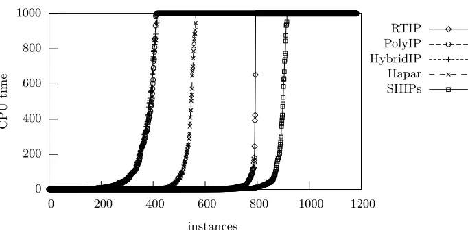
Fig. 1.Relative performance of HIPP solvers
2
Haplotype Inference by Pure Parsimony
A haplotype is the genetic constitution of an individual chromosome. The
un-derlying data that forms a haplotype is generally viewed as the set of SNPs in a given region of a chromosome. Normal cells of diploid organisms contain two haplotypes, one inherited from each parent. The genotype represents the con-flated data of the two haplotypes. The value of a particular SNP may be A, B or A/B, depending on whether the organism is homozygous with allele A, homozygous with allele B or heterozygous.
Starting from a set of genotypes, the haplotype inference by pure parsimony problem consists in finding a minimum set of haplotypes that can be used to derive, by pairwise combinations, the given set of genotypes.
Given a set G of n genotypes, each of length m, the haplotype inference problem consists in finding a setHof 2·nhaplotypes, not necessarily different, such that for each genotype gi ∈ G there is at least one pair of haplotypes (hj, hk), withhj andhk ∈ Hsuch that the pair (hj, hk) explainsgi. The variable
ndenotes the number of individuals in the sample, andm denotes the number of SNP sites. gi denotes a specific genotype, with 1 ≤i ≤n. Furthermore,gij denotes a specific sitej in genotypegi, with 1≤j≤m.
Table 1.Classes of instances used: number of SNPs and genotypes
Class # InstancesminSNPsmaxSNPsminGENsmaxGENs
ms 380 4 57 9 94
phasing 329 14 188 34 90
hapmap 24 4 29 5 68
biological 450 4 77 4 49
Total 1183 4 188 4 94
values 0 or 1, depending on whether both haplotypes have value 0 or 1 at that site, respectively. Heterozygous sites are represented by value 2.
The HIPP problem is to find a minimum-size setHof haplotypes that explain all genotypes inG. For example, consider the set of genotypes: 2120, 2120 and 1221. There are solutions for this example that use six distinct haplotypes, but solution 0100/1110, 0100/1101, 1011/1101 uses only four distinct haplotypes.
Two strings (denoting genotypes or haplotypes) areincompatibleif and only if the strings have at least one site where one string has value 1 and the other string has value 0. Otherwise the strings are said to becompatible.
A comparison of the performance of alternative approaches to the HIPP problem is summarized in Figure 1. A universe of 1183 problem instances is used, from which 854 instances were taken from [12] and the remaining (harder) instances are described by Schaffner [15] and correspond to the SU-100kb, SU1, SU2 and SU3 classes available fromhttp://www.stats.ox.ac.uk/∼ marchini-/phaseoff.html. All problem instances were simplified in a preprocessing step, according to what has been suggested in [2]: duplicated genotypes and sites were removed, as well as complemented sites. For each class, Table 1 gives the number of instances, and the minimum and maximum number of SNPs and genotypes, respectively, after removing duplicated genotypes and duplicated and complemented sites. Themsclass includes the uniform and nonuniform classes of instances that have been used in [2] but extended with additional, more complex, problem instances. Thephasinginstances correspond to the instances described in [15] which were generated to evaluate phasing algorithms. Thehapmapclass of instances is also the one used in [2]. Finally, the instances for the biological class were generated from publicly available data (e.g. [14, 4, 3, 9]).
The HIPP solvers RTIP [6], PolyIP [1], HybridIP [2], Hapar [18] and SHIPs [12] were considered1
. The run times for each solver were sorted and plotted, the cut-off point being 1000 seconds. All results shown were obtained on a 1.9 GHz AMD Athlon XP with 1GB of RAM running RedHat Linux. For the ILP-based HIPP solvers, the ILP package used was CPLEX version 7.5. As can be concluded, SHIPs is the HIPP tool capable of solving the largest number of problem in-stances. SHIPs aborts 268 problem instances out of 1183 instances, whereas RTIP aborts 389 instances, Hapar aborts 619 instances, HybridIP aborts 767 instances and PolyIP aborts 771 instances. Nonetheless, we should note that
1
95% of the problem instances aborted by RTIP were aborted due to memory ex-haustion. Hence, RTIP may be competitive for solving some problem instances but it is not a robust solver.
3
Solving ILP HIPP Models with PBO
This section reviews existing ILP models for the HIPP problem [7, 10]. In addi-tion, the section includes results using a modern Pseudo-Boolean Optimization (PBO) solver instead of a standard ILP solver.
In a pseudo-Boolean formula, variables have Boolean domains and constraints are linear inequalities with integer coefficients,
X
cixi≥n ci, n∈Z, xi∈ {0,1}. (1)
For example,x+ 2y−z≥2 is a pseudo-Boolean constraint (also denoted as PB-constraint). From an ILP point of view, PB-constraints can be seen as a special-ization of ILP where all variables are Boolean. This problem formulation is also known as 0-1 integer programming. From a SAT point of view, PB-constraints can be seen as a generalization of clauses. Furthermore, a pseudo-Boolean for-mula can be extended with an optimization function.
3.1 Exponential-Size ILP Models
The first ILP model proposed for the HIPP problem,RTIP [6], has linear space complexity on the number of possible haplotypes and, therefore, it is exponential on the number of given genotypes.
A Boolean variableyi,uis associated with each pairuof haplotypes that can explain a given genotypegi, and denotes whether this pair of haplotypes is used for explaininggi. A cardinality constraint,
X
u
yi,u= 1, (2)
requires that exactly one pair of haplotypes must be used for explaining each genotype, among all pairs that can explain the genotype. Each candidate haplo-type is associated with a dedicated variablexv, such thatxv= 1 if the haplotype is used. The utilization of a specific pair of haplotypes for explaining a genotype (i.e.yi,u= 1) implies the respectivexv variable,
yi,u→xv, (3)
for each haplotype in the pair. The cost function is used to minimize the number of haplotypes used,
minimizeXxv. (4)
yi,uis such that they are not part of any other pair of haplotypes, then theyi,u variable and the related xv variables can be removed from the formulation. A key drawback of the RTIP model is that the number of candidate haplotypes grows exponentially with the number of heterozygous sites. Hence, RTIP does not scale for large problem instances.
The RTIP model inspired a branch-and-bound algorithm to the HIPP prob-lem, known asHapar [18].
3.2 Polynomial-Size ILP Models
A more recent ILP model, PolyIP [1], is polynomial in the number of sites m
and population sizen, with a number of constraints and variables, respectively, in Θ(n2
m) and Θ(n2
+n m). The PolyIP model represents the 2·ncandidate haplotypes as sequences of Boolean variables, and then establishes conditions for the haplotypes to explain the corresponding genotypes, such that the total number of distinct haplotypes is minimized. Haplotypes are represented with Boolean variables yi j, 1 ≤i ≤2nand 1≤j ≤m, i.e.m variables for each of the 2·ncandidate haplotypes.
First, the PolyIP model defines conditions on the sites, with 1≤i≤nand 1≤
j≤m,
y2i−1j= 0 andy2i j = 0,ifgij = 0,
y2i−1j= 1 andy2i j = 1,ifgij = 1,
y2i−1j+y2i j = 1 ifgij = 2,
(5)
wheregij ∈ {0,1,2}denotes the possible values at each site. Second, the PolyIP model defines conditions for identifying different haplotypes, with 1 ≤l ≤i ≤ 2nand 1≤j≤m. Boolean variabledl i is defined such that dl i= 1 ifhi6=hl. The resulting conditions become
yi j−yl j≤dl i,
yl j−yi j ≤dl i. (6)
If at least one site ofhi andhldiffers, thendl i needs to be assigned value 1. Third, the model introduces thexivariables, denoting whetherhiis different from all previous haplotypeshl, where 1≤l < i, and defines conditions on these variables. Each Boolean variablexiis defined such thatxi= 1 ifhiis unique with respect to the previous haplotypes. Thus, ifhi is unique, then
Pi−1
l=1dl i=i−1; otherwisePil=1−1dl i< i−1. As a result, the condition on variablexi becomes
xi ≥2−i+ i−1 X
l=1
dl i. (7)
Finally, the cost function minimizes the number of different haplotypes,
minimize 2n P i=1
0 200 400 600 800 1000
0 200 400 600 800 1000 1200
CPU
time
instances
Class all with 1183 instances
[image:7.595.140.485.138.314.2]PolyIP PolyPB SHIPs
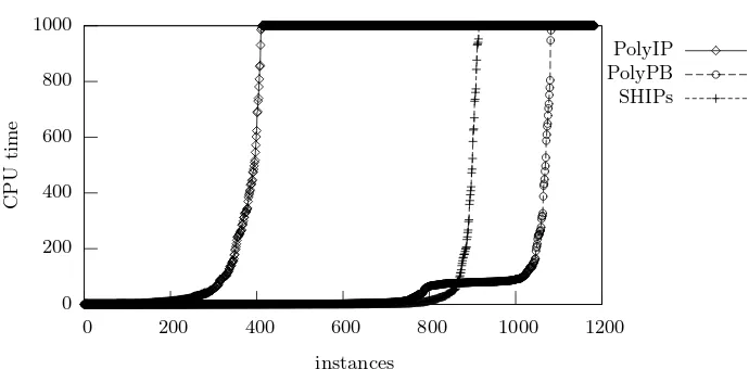
Fig. 2.Relative performance of PolyIP, PolyPB and SHIPs
A number of optimizations have been proposed to the basic PolyIP model [1], with the purpose of improving the quality of the LP relaxation step of standard ILP solvers, and therefore pruning the search space to be handled by the ILP solver.
More recently, the same authors introduced a new polynomial-size formula-tion,HybridIP [2], representing a hybrid of the RTIP and PolyIP formulations. Nevertheless, existing experimental results (see Figure 1) suggest that the per-formance of the two polynomial models does not differ significantly.
3.3 ILP vs. PBO Solvers
As is clear from the description of the ILP models, all variables are Boolean and all coefficients are integer. Hence, the HIPP ILP models are also PBO mod-els, and so PBO solvers can be considered. The results summarized in Figure 1 indicate that the performances of the PolyIP and HybridIP models are sim-ilar. Moreover, the RTIP model is known to be inadequate for larger problem instances, due to the exponential growth of the model in the number of heterozy-gous sites per genotype. As a result, this section only evaluates the performance of the PolyIP model using a PBO solver (hereafter referred to as PolyPB). The PBO solver MiniSAT+ [5] is used on all reported PBO results. Although other PBO solvers analyzed in [13] were considered, MiniSAT+ was by far the most efficient.
10−2
10−1
100
101
102
103
10−2 10−1 100 101 102 103
SHIPs
[image:8.595.188.365.109.289.2]PolyPB
Fig. 3.Run times for PolyPB and SHIPs
by iteratively calling the SAT solver where for each new iteration the objec-tive function is updated until the problem is unsatisfiable. For example, given a minimization problem with an objective functionf(x), MiniSAT+ first runs the solver on the set of constraints (without considering the objective function) to get an initial solutionf(x0) =k. Then it adds the constraintf(x)< k and runs the solver again. If the problem is unsatisfiable, thenkis the optimum solution. If not, the process is repeated with the new smaller solution. Observe that trans-lating to SAT results in an approach that is particularly suited for problems that are almost pure SAT. Indeed, this is the case for the HIPP problem. Hence, one may expect to get a faster procedure with MiniSAT+ than by applying a native PBO solver, not optimized towards propositional SAT.
Figure 2 compares the PolyIP model using the CPLEX solver, the PolyPB model using the PBO solver MiniSAT+ and the SHIPs solver on the 1183 prob-lem instances described in Table 1 for a timeout of 1000 seconds. Clearly, PolyPB outperforms SHIPs in terms of the number of instances solved. Although both solvers are able to solve the majority of the 1183 problem instances within 1000 seconds, PolyPB only aborts 100 instances whereas SHIPs aborts 268 instances. Observe that PolyIP is significantly worse, aborting 771 out of 1183 instances.
10−2
10−1
100
101
102
103
10−2 10−1 100 101 102 103
Without
symmetry
breaking
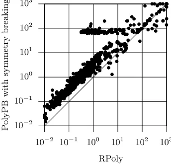
[image:9.595.190.362.122.288.2]With symmetry breaking
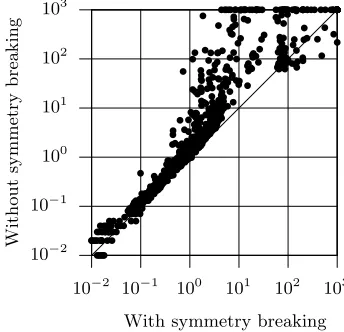
Fig. 4.Run times for PolyPB with and without symmetry breaking
more robust than SHIPs. Finally, there are still 84 instances that both solvers are unable to solve within 1000 seconds.
4
RPoly: an Optimized PolyPB Model
Although the results shown in the previous section are promising, it is possible to further optimize the PolyPB model. Indeed, SHIPs is still showing a better performance in a large number of problem instances, which motivates the in-corporation of some of the SHIPs model features into the PolyPB model. This section addresses optimizations to the PolyPB model with the main goal of re-ducing the run times.
These optimizations are two-fold: (1) the elimination of key symmetries and (2) the reduction of the size of the model. It is well-know that the SHIPs model would not be competitive if it was not for some specific optimizations, which include breaking key symmetries. Symmetries are broken by adding constraints to the model. We have also observed that the PBO instances generated with the PolyPB model are significantly larger than the SAT instances generated with the SHIPs model. The number of constraints in the PBO model can be up to an order of magnitude larger than the number of constraints in the SAT model, whereas the number of variables in the PBO model can be up to a factor of 3 larger than the number of variables in the SAT model.
The resulting model is referred to asReduced Poly model (RPoly).
4.1 Eliminating Key Symmetries
to a HIPP problem were a genotype gi is explained by the pair of haplotypes (h2i−1,h2i), the same genotype gi may also be explained by the pair of haplo-types (h2i,h2i−1). Eliminating this symmetry significantly reduces the number of solutions and consequently reduces the search space.
In practice, this kind of symmetry is eliminated by adding additional con-straints to the model, which guarantee that the elements in a pair of haplotypes are lexicographically ordered. Hence, for each sitegij in a genotypegi we must force the following:
– Ifgi j= 2 and gi j0 6= 2 (∀j0:j0 < j), theny2i−1j−y2i j <0.
Figure 4 compares the performance of the PolyPB model with and without symmetry breaking constraints. Clearly, with a few exceptions (72 out of 1183 in-stances), eliminating symmetries accelerates the performance of the PBO solver. The new model is faster than the PolyPB model for 90% of the instances and up to 2 orders of magnitude. This result comes as no surprise, given the success of the same technique when implemented in the SHIPs model. This result is in-deed significant, as the new model only aborts 47 instances, whereas the PolyPB model aborts 100 instances.
4.2 Reducing the Model
The organization of RPoly follows the organization of PolyIP: two haplotypes are associated with each genotype, and conditions are defined which capture when a different haplotype is used for explaining a given genotype. However, RPoly has a few key differences. First, the set of variables is different. Instead of associating a variable with each site of each haplotype, RPoly only associates variables with heterozygous sites (since the value of haplotypes in the other sites is known beforehand, and so can be implicitly assumed). In addition, each used variable describes the possible pairs of values for the corresponding heterozygous site.
In practice, the model associates two haplotypes,ha i andh
b
i, with each geno-type gi, and these haplotypes are required to explain gi. Moreover, the model associates a variable ti j with each heterozygous site (i, j) (i.e. with gi j = 2). Hence, ti j = 1 indicates that hai j = 1 and hbi j = 0, whereas ti j = 0 indicates that ha
i j = 0 and hbi j = 1 2
. The value of ha
i and hbi at homozygous sites j is implicitly assumed.
This alternative definition of the variables associated with the sites of geno-types reduces the number of variables by a factor of 2. In addition, the model only creates variables for heterozygous sites, and, therefore, the number of vari-ables associated with sites equals the total number of heterozygous sites. As a result, the conditions provided by expression (5) are eliminated. It should also be mentioned that this definition of the variables associated with sites follows the SHIPs model [11, 12].
2
Hence, the symmetry in a pair of haplotypes is broken by considering thattij = 0
Finally, another key modification is that the candidate haplotypes for each genotype are related with candidate haplotypes for other genotypes only if the two genotypes are compatible. Clearly, incompatible genotypes are guaranteed not to be explained by the same haplotype.
The proposed modification implies the use of two additional sets of variables. Variable xp qi
1i2, with p, q ∈ {a, b}and 1 ≤ i2 < i1 ≤n, is 1 if the phaplotype
of genotype i1 and the qhaplotype of genotype i2 are incompatible. Clearly, if genotypesi1 and i2 are incompatible, then the value of x
p q
i1i2 is 1 for the four possible combinations ofpandq. Moreover, two genotypesi1andi2are related only with respect to sitesj such that either gi1 or gi2 is heterozygous at that site. In addition, the model uses variables to denote when one of the haplotypes associated with a given genotype is different from all previous haplotypes. Hence,
upi, withp∈ {a, b}and 1≤i≤n, is 1 if haplotypepof genotypei is different from all previous haplotypes.
The conditions on the upi variables are based on the conditions for the xi variables for the PolyIP model,
^
1≤k<i
(xp ai k∧xp bi k)→upi. (9)
The conditions on the xp qi1i2 variables are all of the following form, for all 1≤j ≤m:
¬(R↔S)→xp qi
1i2, (10)
where the predicatesRandSdepend on the values of the sites (i1, j) and (i2, j), and on which of the haplotypes is considered, i.e., either a or b. Observe that 1 ≤ i2 < i1 ≤ n, 1 ≤ j ≤ m, and p, q ∈ {a, b}. Accordingly, the R and S predicates are defined as follows:
– Ifgi1j6= 2, then R= (gi1j ↔(q↔a)) andS=ti2j.
– Ifgi2j6= 2, then R= (gi2j ↔(p↔a)) andS=ti1j.
– Ifgi1j= 2∧gi2j = 2, thenR=¬(p↔q) andS=¬(ti1j ↔ti2j). Finally, the cost function is given by
minimize n X
i=1
(uai +u b
i). (11)
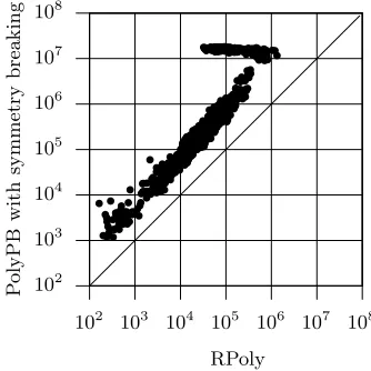
The proposed modifications result in significantly smaller PBO problem in-stances. Figure 5 compares the number of terms for the PolyPB and the RPoly models. The results are consistent and show that the number of terms in RPoly is a factor of 5 to 10 smaller than in PolyPB. Albeit not shown, the number of variables in RPoly can be up to a factor of 3 smaller than the number of variables in PolyPB. We should note that thephasingclass of instances exhibits a different behavior: most of these instances have around 107
102
103
104
105
106
107
108
102
103
104
105
106
107
108
P
olyPB
with
symmetry
breaking
[image:12.595.190.357.121.288.2]RPoly
Fig. 5.Number of terms for PolyPB and RPoly
have a higher number of incompatible genotypes when compared with the other classes of instances. Hence, the impact of the reduced model is much more signif-icant. For the same reason, the impact on the run times is also more significant (see Figure 6 where the run time for thephasinginstances using the PBO model with symmetry breaking is around 102
seconds). As a result, for these instances RPoly can outperform PolyPB by two orders of magnitude.
Finally we evaluate the effect of the reductions described above with respect to the run times. Figure 6 compares the PolyPB model extended with sym-metry breaking constraints and the RPoly model, both using the PBO solver MiniSAT+, on the set of 1183 problem instances and with a timeout of 1000 seconds. With a few exceptions (28 out of 1183 instances), RPoly is consistently faster than PolyPB, and the speedup can reach 2 orders of magnitude. The few exceptions where RPoly is slower are explained by the branching heuristics used by MiniSAT+, which, in some cases, may not select the most adequate variables to branch on.
4.3 RPoly vs. SHIPs
In this section we measure the progress made with this work, by comparing the SHIPs model [12] with the RPoly model. The RPoly model is based on the PolyIP model but uses a PBO solver, MiniSAT+, and introduces key optimizations: the elimination of symmetries between the elements within a pair of haplotypes and the reduction on the size of the model.
num-10−2
10−1
100
101
102
103
10−2 10−1 100 101 102 103
P
olyPB
with
symmetry
breaking
[image:13.595.191.363.123.288.2]RPoly
Fig. 6.Run times for PolyPB with symmetry breaking and RPoly
ber of genotypes, and iteratively reduces the number of different haplotypes until a solution with a minimum number of different haplotypes is found.
Figure 7 compares the RPoly model using the PBO solver MiniSAT+ and the SHIPs solver. For a small number of problem instances (52 out of 1183) SHIPs is faster than RPoly, and the speedup can reach 2 orders of magnitude. However, for most problem instances (1089 out of 1183), RPoly is faster than SHIPs. It should be observed that SHIPs is, in general, slower on very easy problem instances, essentially due to the initial setup time [11]. Nevertheless, the results also clearly show that RPoly is significantly more robust than SHIPs. RPoly aborts on a significantly smaller number of instances, being able to solve more than 96% of the problem instances. Finally, observe that only two instances aborted by RPoly can be solved by SHIPs.
5
Conclusions and Future Work
10−2
10−1
100
101
102
103
10−2 10−1 100 101 102 103
SHIPs
[image:14.595.190.365.112.289.2]RPoly
Fig. 7.Run times for RPoly and SHIPs
The results indirectly suggest that the performance improvements obtained with SHIPs [11, 12] are to a large extent explained by the efficiency of modern SAT solvers. Indeed, SAT-inspired PBO solvers obtain extremely good results with PolyIP and with RPoly, which are PBO models that differ significantly from the SHIPs SAT-based approach. In addition, the different PBO models provide a new, relevant, and essentially endless, source of challenging real problem in-stances for PBO solvers.
Despite the promising results obtained using MiniSAT+ with the RPoly model, several challenges remain. A number of problem instances cannot be solved by any HIPP solver. In addition, larger HIPP instances are expected to be significantly more challenging.
Finally, we should mention that having a competitive HIPP solver allows us to extend the pure parsimony approach with some ideas which are on the basis of other haplotype inference approaches. This will enable us to develop parsimony-based methods that explicitly incorporate genetic models (e.g. as in Phase [16]), with the objective of improving the accuracy of the reconstructed haplotypes.
Acknowledgments This work is partially supported by Funda¸c˜ao para a Ciˆencia e Tecnologia under research project POSC/EIA/61852/2004 and PhD grant SFRH/BD/28599/2006, and by INESC-ID under research project SHIPs.
References
2. D. Brown and I. Harrower. Integer programming approaches to haplotype
infer-ence by pure parsimony. IEEE/ACM Transactions on Computational Biology and
Bioinformatics, 3(2):141–154, 2006.
3. M. J. Daly, J. D. Rioux, S. F. Schaffner, T. J. Hudson, and E. S. Lander. High-resolution haplotype structure in the human genome.Nature Genetics, 29:229–232, October 2001.
4. C. M. Drysdale, D. W. McGraw, C. B. Stack, J. C. Stephens, R. S. Judson, K. Nandabalan, K. Arnold, G. Ruano, and S. B. Liggett. Complex promoter and coding regionβ2-adrenergic receptor haplotypes alter receptor expression and
predict in vivo responsiveness. InProceedings of the National Academy of Sciences of the United States of America, volume 97, pages 10483–10488, September 2000. 5. N. E´en and N. S¨orensson. Translating pseudo-Boolean constraints into SAT.
Jour-nal on Satisfiability, Boolean Modeling and Computation, 2:1–26, March 2006. 6. D. Gusfield. Haplotype inference by pure parsimony. In14th Annual Symposium on
Combinatorial Pattern Matching (CPM’03), volume 2676, pages 144–155, February 2003.
7. D. Gusfield and S. Orzach. Handbook on Computational Molecular Biology, vol-ume 9 ofChapman and Hall/CRC Computer and Information Science Series, chap-ter Haplotype Inference. CRC Press, December 2005.
8. B. Halld´orsson, V. Bafna, N. Edwards, R. Lippert, S. Yooseph, and S. Istrail. A survey of computational methods for determining haplotypes. In Proceedings of the First RECOMB Satellite on Computational Methods for SNPs and Haplotype Inference, volume 2983 ofLNBI, pages 26–47, February 2004.
9. D. L. Kroetz, C. Pauli-Magnus, L. M. Hodges, C. C. Huang, M. Kawamoto, S. J. Johns, D. Stryke, T. E. Ferrin, J. DeYoung, T. Taylor, E. J. Carlson, I. Herskowitz, K. M. Giacomini, and A. G. Clark. Sequence diversity and haplotype structure in the human ABCD1 (MDR1, multidrug resistance transporter). Pharmacogenetics, 13:481–494, November 2003.
10. G. Lancia, C. M. Pinotti, and R. Rizzi. Haplotyping populations by pure
parsi-mony: complexity of exact and approximation algorithms. INFORMS Journal on
Computing, 16(4):348–359, March 2004.
11. I. Lynce and J. Marques-Silva. Efficient haplotype inference with Boolean satisfi-ability. InNational Conference on Artificial Intelligence (AAAI), July 2006. 12. I. Lynce and J. Marques-Silva. SAT in bioinformatics: Making the case with
hap-lotype inference. InInternational Conference on Theory and Applications of Sat-isfiability Testing (SAT), pages 136–141, August 2006.
13. V. Manquinho and O. Roussel. The first evaluation of Pseudo-boolean solvers (PB’05). Journal on Satisfiability, Boolean Modeling and Computation, 2:103–143, March 2006.
14. M. J. Rieder, S. T. Taylor, A. G. Clark, and D. A. Nickerson. Sequence variation in the human angiotensin converting enzyme. Nature Genetics, 22:59–62, May 1999. 15. S. Schaffner, C. Foo, S. Gabriel, D. Reich, M. Daly, and D. Altshuler. Calibrating a coalescent simulation of human genome sequence variation. Genome Reasearch, 15:1576–1583, November 2005.
16. M. Stephens, N. Smith, and P. Donelly. A new statistical method for haplotype reconstruction.American Journal of Human Genetics, 68:978–989, February 2001. 17. The International HapMap Consortium. A haplotype map of the human genome.
Nature, 437:1299–1320, October 2005.