Multifractal modelling of liquid water clouds : cloud spatial structure and its effect on the solar radiation field

(1)

MULTIFRACTAL MODELLING OF LIQUID

WATER CLOUDS:

CLOUD SPATIAL STRUCTURE AND ITS

EFFECT ON THE SOLAR RADIATION FIELD

by

Kurt S. Fienberg, B.Sc.(Hons)

C

Submitted in fulfilment of the

requirements for the degree of

Doctor of Philosophy

University of Tasmania (August, 2003)

(2)

/ 28 August 2003

Declaration

I

hereby declare that this thesis contains no material that has been accepted for the award of any other degree or diploma in any tertiary institution, and to the best of my knowledge contains no copy, paraphrase or material previously published or written by another person, except where due reference is given in the text.

I

28 August 2003

Authority of access

(3)

Abstract

At any point in time a significant fraction of the globe is covered by liquid water clouds. Understanding the relationship between cloud and solar radiation is therefore of great importance for both climate modelling and remote sensing. Previous studies have found that cloud spatial structure has a significant effect on cloud albedo, with spatial inhomogeneities leading to less reflection of solar radia-tion than was predicted by the tradiradia-tional homogeneous cloud model. This thesis investigates further the consequences of cloud spatial variability on atmospheric radiation, with the aim of developing methods to improve radiation modelling and remote sensing of cloud properties.

The basis of this study is the quantification of the scaling and intermittency of liquid water fields using a multifractal model. The fractionally integrated flux (FIF) model is used to both describe and numerically simulate cloud fields, with model parameters being determined from aircraft measurements made during 98 flights over northern Tasmania, Australia. The aircraft data set is divided into three broad cloud types: stratocumulus, altostratus and low level cumulus. The horizontal fluctuations in all three cloud types are shown not only to be scale invariant and non-stationary, but also to have very similar statistics with only one out of three model parameters varying significantly between cloud types.

Clouds with horizontal structure described by the FIF model but constant ver-tical profiles are then used in Monte Carlo radiative transfer calculations. The differences between the multifractal and homogeneous cloud results are larger than those previously reported for marine stratocumulus, due to the larger degree of inhomogeneity in the cloud types considered. The results of the Monte Carlo simu-lations are used to derive the "effective optical properties" of the multifractal cloud fields, defined as the optical properties of a homogeneous cloud producing the same radiative transfer results as the multifractal cloud. This allows the well-known and efficient radiative transfer techniques for homogeneous cloud to be applied to mul-tifractal cloud. The effective optical properties were found to vary with the spatial scale under consideration, and an empirical parameterisation for the effective op-tical properties is presented that is a function of spatial scale, mean cloud opop-tical depth and single-scattering albedo.

(4)

(5)

Acknowledgements

I would like to thank everyone who has assisted me in this doctoral project, including:

• Hydro Tasmania for their funding and support.

• Andrew Lenton, Alex Nazarov, Christina Nebel, Graham Vertiga,n, and Ian Searle for the collection of the aircraft data and other aid.

• My supervisor Manuel Nunez for his consistent interest, guidance, and assis-tance in all aspects of the project.

(6)

3.1 Introduction

3.2 Measured multifractal statistics of liquid water content

48

49 3.2.1 The data set

49 3.2.2 Energy Spectra

51 3.2.3 The universality parameters

57 3.2.4 Diurnal cycle of stratocumulus clouds

64 3.2.5 Annual/Seasonal cycle of stratocumulus clouds

66 3.3 The probability distribution and cloudy fraction

67 3.4 Summary of Chapter 3

77

4 Radiative properties of horizontally multifractal clouds 79

4.1 Introduction

79 4.2 The Cloud and Radiation Models

80 4.2.1 Numerical generation of multifractal cloud fields

80 4.2.2 Monte Carlo radiative transfer calculations

82 4.3 Conservative Scattering Results

83 4.3.1 Definition of the effective optical depth approximation

85 4.3.2 Parameterization of the effective optical depth

90 4.4 Non-Conservative Scattering Results

97 4.4.1 Consistency of the approximations for absorbing clouds

101 4.4.2 Empirical parameterization

104 4.4.3 Error analysis

110 4.5 Accuracy of the approximation under different conditions 112

4.5.1 Varying the asymmetry parameter

112 4.5.2 Varying the fractal model parameters

118 4.5.3 Reflected radiance distributions

124 4.6 Comparison with the EHCA

130

(8)

5 Radiative properties of 3-dimensionally multifractal clouds 135

5.1 The modelling 137

5.2 Conservative scattering results 139

5.3 Non-conservative scattering results 150

5.4 Summary of Chapter 5 158

6 Transmitted radiation under cloudy skies 1 163

6.1 VSP radiance measurements 165

6.1.1 VSP Description 165

6.1.2 Measurement Acquisition 169

6.2 Radiance modelling 170

6.2.1 Cloud optical depth retrieval 172

6.3 Comparison of VSP radiance measurements with model output. 175 6.4 Paranieterisation of multifractal-cloud radiance distribution 179

6.5 Summary of Chapter 6 184

7 Comparison of satellite cloud property retrieval with in situ

mea-surements 186

7.1 Overview 186

7.2 Objective Analysis of Multifractal Fields 188

7.2.1 Method description 190

7.2.2 Numerical Simulation 196

7.2.3 Simulation of upscaling aircraft data 198

7.3 Data Acquisition Methods 200

7.3.1 Satellite Retrieval 202

7.3.2 Aircraft Data 205

7.4 Comparison of results 206

(9)

8 Conclusion 215

8.1 Summary of Results

215 8.1.1 Cloud Spatial Structure

215 8.1.2 Radiation modelling

219

8.1.3 Remote sensing

222

(10)

Chapter 1 Introduction

1.1 Motivations

Low-level, mainly liquid water clouds have been estimated to cover an average of approximately one quarter of the globe [Hartman et al., 1992]. This means

(11)

can cover the wide spatial and temporal scales over which clouds occur in the atmosphere.

In the case of climate modelling, it has long been recognised that a significant proportion of the earth's radiation budget can be attributed to cloud radiative forcing [e.g. Wielicki et al., 1995; Mitchell, 1989]. However, clouds influence the

radiation budget in a variety of ways, both cooling the earth by increasing the albedo of the earth-atmosphere system and heating the earth by lowering the level of outgoing longwave radiation. While cirrus clouds are usually high, cold and optically-thin, and hence have a net heating effect, low level clouds have a net cooling effect because they are optically thick, reflect a relatively large amount of solar radiation, and are warm enough to have little net effect on longwave radiation

[Rossow and Lacis, 1990]. Of these two cases, global radiation studies have found

that the net radiative forcing by clouds is greatest in regions of low level cloud, and that the greatest effect is the reflection of shortwave radiation [Harrison et al.,

1990; Ramanathan et al., 1989; Rossow and Zhang, 1995] . Cahalan et al. [1994a]

estimated that a 10% change in the global average albedo of stratocumulus cloud would produce a 5°C change in the equilibrium surface temperature, equivalent to the change in surface temperature since the last ice age. From another point of view, this means that if global circulation models are incorrect in their predictions of liquid water cloud albedo then surface temperature predictions would contain significant errors. This is particularly important when considering that not only do clouds affect the climate but also changes in climate can affect cloud formation - clouds are formed by dynamic atmospheric processes affected by global warming or cooling [Rogers and Yau, 1989] leading to a range of possible feedback mechanisms.

This makes accurate cloud modelling necessary for research into climate change.

(12)

of cloud on the radiation budget. These include: global surveys of cloud properties to develop cloud climatologies [e.g. Han et al., 1994; Kawamoto et al. 2001]; the estimation of rain rates and precipitation area [e.g. Lensky and Rosenfield, 1997]; the investigations of the effects of weather modification through cloud-seeding [e.g. Sassen and Zhao, 1993]; the estimation of radiation levels at the surface [e.g. Pinker et al., 1995]; the validation or initiation of numerical cloud models [e.g. Fouilloux and Iaquinta, 1997]. Because of the vantage point they occupy, high above the earth's surface, satellite platforms are able to cover a wider range of spatial scales than ground based or aircraft measurements. This is of great advantage in measurement programs involving liquid water clouds because, as will be examined later in this thesis, their properties and structure fluctuate widely over a wide range of scales [Davis et al., 1996a]. Many techniques for the remote sensing of cloud properties have been developed and they utilise many wavelengths of radiation from radar [e.g. Belton et al., 1980; Lin et al., 2002], through microwave [e.g. Simmer et al. 1989] and thermal infrared [e.g. Liou et al., 1990], to the solar spectrum [e.g. Nakajima and King, 1990]. However, the scope of this work is restricted to the last of these, as the bulk of global cloud data is obtained from satellite observations of reflected solar radiation.

1.2 Radiative transfer under cloudy conditions

(13)

model is known as the plane-parallel homogeneous (PPH) cloud model. However, real clouds do not conform to the PPH model, and this has consequences for ra-diative transfer. Clouds with inhomogeneous liquid water fields have been found to have a significantly lower average reflectance (and higher average transmittance) than a PPH cloud field with the same mean liquid water content, if the observa-tion scale under consideraobserva-tion exceeds a photon mean-free-path length [Davis et

(14)

culation methods for radiation in inhomogeneous cloud fields - such as Monte Carlo radiative transfer [Marchuk et al., 1980], the diffusion approximation approach [e.g. Cu and Liou, 2001], or the spherical harmonic discrete ordinate method [Evans,

1998] - are generally much more time consuming.

Several faster, approximate methods of radiative transfer have been developed for these applications. The first is the independent pixel approximation (IPA)

[Cahalan et al., 1994b], in which PPH cloud calculations are performed for pixels

at a scale equal to or smaller than a photon mean-free path length, and then these results are averaged over whatever scale is being considered. The IPA avoids the effects of sub-pixel scale variability because liquid water content variability at scales smaller than the mean free path length does not have a significant effect on the radiation field [Marshak et al., 1998]. The area averaging then reduces the error

due to horizontal transport of radiation. If the area under consideration is small enough that horizontal transport of photons is significant, the variant known as the non-local IPA (NIPA) [Marshak et al., 1996] may be used instead to take this

into account. There is no particular cloud model inherent in the IPA, so some cloud model must be chosen to determine the distribution of the cloud liquid water content. Calculations performed using the IPA are much faster than Monte Carlo radiative transport code, but if the pixels or grids under consideration are at the " meso-scale (or larger) the IPA calculations are still many times slower than PPH calculations, because they effectively require tens or hundreds of PPH calculations per grid point.

(15)

(16)

1.3 Cloud spatial structure and the approach taken

in this thesis

To implement any of these radiative transfer schemes, an accurate model of cloud structure is required. Over the last two decades the need for a realistic cloud model for radiative transfer has led various researchers to investigate cloud spatial structure and to develop inhomogeneous cloud models. This has occurred along side a general recognition that atmospheric structures and processes occur over a wide range of scales, and as part of the development of a paradigm of scale invariance and (multi)fractal analysis. Lovejoy [1982] first suggested that cloud spatial distributions could be modelled as a fra,ctal structure. Various measurements since then, including Cahalan and Joseph [1989], Malinowski and Zawadzki [1993], and Davis et al. [1996a], have shown that cloud structure is scale invariant, and hence that a fractal model is applicable. These studies have generally concentrated on overcast marine stratocumulus cloud. Multifractal analyses to further quantify the intermittency of cloud liquid water content have been performed [Davis et al., 1994; Marshak et cd.,1997], also on marine stratocumulus. In this study an attempt is made to significantly extend this data set and begin a move toward a more complete climatology of cloud internal structure.

A range of multifractal models have been developed to describe scale invari-ant processes, including the lognormal model [Kolmogorov, 1962] and the bounded cascade model [Cahalan, 1989; Cahalan et at., 1994a]. For thorough reviews of mul-tifractal modelling and analysis, the reader is referred to Schertzer and Lovejoy

(17)

[e.g. Wilson et al., 1991], as well as for modeling other atmospheric quantities in the "unified scaling model" of the atmosphere [Schertzer and Lovejoy,1985; Chin-girinskaya et al., 1994; Lovejoy and Schertzer, 1995a]. The FIF model has the advantages over other multifractal models of being able to be adjusted to a wider range of statistics [Davis et al., 1994] and of being based on the symmetries of the equations governing atmospheric turbulence. While in general multifractals could require an infinite number of parameters to completely define them, this model posits that atmospheric phenomena fall into universality classes of multifractals defined by three parameters. These are stable, attractive multifractal processes. Although there has been some debate about the mathematical existence of these classes due to a possible divergence in the small scale limit, this seems to be re-solved by taking alternate routes to universality - see Schertzer and Lovejoy [1997] for details.

Measurements have shown, for example, that turbulent velocity fields [Chin-girinskaya et al., 1994; Lazarev et al., 1994] and rain radar reflectivities [Tessier et al., 1993; Lovejoy and Schertzer, 1995] can be described by these universality classes. Analysis of cloudy satellite images have shown that the statistics of cloud radiances also closely fit these universal multifractals [Lovejoy et al., 1993; Tessier

et al., 1993; Lovejoy et al., 2001a]. However, the FIF model has not yet been fitted to direct in situ measurements of cloud liquid water content. This is of importance considering the non-linear relationship between liquid water content and the radi-ation field, and between liquid water content and precipitradi-ation. This is highlighted by the fact that when examining satellite images of cloudy atmospheres, Tessier et al. [1993] found different values for the FIF parameters at different wavelengths.

(18)

to directly determine the FIF model parameters for three different categories of liquid water clouds. In this manner multifractal analysis is extended to cloud types other than the marine stratocumulus that have been the focus of previous analysis. Subsequently, the radiative properties of such multifractal clouds are investigated, with an eye to determining if there are differences between these clouds, described by the FIF model, and those previously examined using the bounded cascade model (with marine stratocumulus parameters). An effective properties approximation is developed for use in radiative transport calculations, in an approach similar to that taken by

Szczap et al.

[2000a;b;c] in developing the EHCA. As in the

EHCA, the focus is on meso-scale pixels suitable for moderate resolution remote sensing or regional climate models. However, this approach is expanded to other liquid water clouds apart from overcast marine stratocumulus, and to include a direct dependence on pixel or grid size. The effects of such an approximation on some applications, such as the remote sensing of cloud properties or determining radiation at the surface, are also examined, as are the radiative implications of vertical variations in the liquid water field.

1.4 Thesis structure

The general goal of this work is therefore to improve the understanding of cloud spatial structure and determine how this knowledge can be used in radiative transfer applications, such as existing climate models and remote sensing algorithms. With this is mind, the structure of the thesis is given as follows:

(19)

Monte Carlo radiative transfer model used to determine the radiative prop-erties of multifractal clouds. Also presented in this chapter is a summary of multifractal statistics and analysis. In general, chapter 2 describes the major tools and methods used later in the thesis.

• Chapter 3 focuses on the analysis of the in situ measurements of cloud liquid water fields. The data is shown to fit the multifractal model and the associated multifractal parameters are empirically determined for three different cloud types. The diurnal and seasonal variation in stratocumulus spatial structure is also examined in this chapter.

• Chapter 4 is a presentation of the results of radiative transfer calculations carried out using clouds with horizontal spatial inhomogeneities described by the FIF model, but with a homogeneous vertical structure. The effective opti-cal properties of both absorbing and non-absorbing clouds are parameterised, and the accuracy of the parameterisation under different conditions is tested. A comparison of our results with the EHCA is also made.

• Chapter 5 describes the results of radiative transfer through clouds with a multifractal structure in the vertical as well as horizontal dimensions, in order to determine the errors that result from the earlier assumption of vertical homogeneity.

(20)

the same total transmittance, and these results are compared to radiometric measurements.

• Chapter 7 presents a comparison of cloud properties derived from satellite remote sensing with those found from in situ measurements. The result of us-ing the effective optical properties approximation in cloud property retrieval, instead of the PPH model alone, is examined. Also investigated is the impact of multifractal cloud structure on the comparison of data sets measured at different resolutions.

• Chapter 8 concludes this thesis and contains a summary of results, as well as recommendations for further study.

(21)

Chapter 2 Cloud and Radiation Models

Many of the results that appear later in this thesis are produced in the framework of two key models: the FIF multifractal model that describes the spatial statistics of the cloud liquid water content field, and the Monte Carlo simulations that calculate the radiative properties of clouds given their spatial structure. In this chapter these two models are described, along with the analysis technique used to determine the parameters of the multifractal model from measured cloud fields, and the numerical method used to generate cloud fields.

2.1 The multifractal cloud model

(22)

choice for phenomenological or statistical modelling. The original fra,ctals used to model clouds and rain were monofractal models [e.g. Mandelbrot 1983] - geomet-ric models containing 'simple' scaling which is characterized by a single (generally non-integer) fractal dimension. However, this approach has been found to be in-sufficient to fully describe the statistics of cloud fields [Davis et al. 1994; Schertzer

and Lovejoy 1985] and multifractal models which require multiple parameters to describe their scaling behavior have been developed. For a more general review of multifra.ctal models see Davis et al. [1990] and for multifractal modelling applied to remote sensing applications see Lovejoy et al. [2001b].

It should also be noted that in this work all scaling is assumed to be isotropic, that is the scaling is assumed to be the same in all dimensions. This assumption is made because the primary data set examined here is one dimensional horizontal aircraft flight data, and hence the data is not available to analyse any anisotropy of scaling, or to implement the framework of generalised scale invariance developed by Schertzer and Lovejoy [1987;1991].

2.1.1 The cascade process

The universal FIF multifractal model [Schertzer and Lovejoy, 1987; 1991] which is used here, was developed out of the theory of turbulent velocity cascades. It is based on three properties of the (incompressible) Navier-Stokes equations that govern atmospheric turbulence: 1) scaling symmetry or invariance under dilations

(zooms); 2) conservation of a quantity with changes of scale - the energy flux, E,

(23)

being made up of substructures on a smaller scale, which are in turn made up of even smaller structures, and so on. This downwards cascade will only end when a scale is reached that is so small that frictional losses of energy dominate, which in the atmosphere is on the order of millimetres. Mathematically, this process can be represented by a multiplicative cascade, where at each step down in scale the substructures are formed by multiplying the parent structure by different (random) factors. That is, if Eeddy is a variable representing a cascade structure at a large

scale then the values of the substructures are given by

Esubeddy = Eeddy•PE, (2.1)

where me is a (stochastic) multiplicative factor. A schematic representation of this

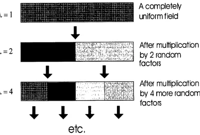
process is shown in Figure 2.1.

In the velocity cascade process, the energy flux E is conserved with the change of

scale but the velocity fluctuations are not. In the model used here this conservation is canonical, i.e. statistical - in the average over the entire ensemble rather than in any particular realisation. Following the convention of labelling the scale under consideration, or resolution, by the ratio

A

L

max

1

(2.2)

where Lmax is the greatest length in a data set and 1 is the length of grid sides at

current scale, then the following scaling relation for the velocity field (v) measured at scale A [Kolmogorov, 1941; Obukhov, 19491:

(24)

The cascade process in one dimension:

2 =1

.7 -..., ,-,-,.-f -,--i•-•,-.+4.

t- - ■ - +.4. , , . f- ..

...1.3....-1.49-...- .

---' ----!-- .14i : ,4 -:--,---+----₁_-_'_-_i

-t-i-r-

.,...1.,..1.4_4.1-1.7.,_,_, _{----t-z-- ,}

1 III • 1._ . , ...-4- .•,---, r. ,---,--,---,-,,,,-,••• .7--*. ,- 1.--r.

A completely

uniform field

2 =4

After multiplication

by 2 random

factors

After multiplication

by 4 more random

factors

[image:24.559.95.497.261.532.2]

4441

etc.

(25)

where Av(l) = v(x + 1) — v(x). So as the cascade process continues from large to small length scales, the velocity fluctuations decrease on average, although the ensemble-mean energy flux is constant. As each area on a larger scale is divided into smaller areas, in the cascade process, the redistribution of energy is uneven, leading at much smaller scales to some (randomly distributed) areas of extremely high values and many others with very little energy or velocity. In this way a very intermittent velocity field is formed.

This model of the spatial distribution of turbulent velocity fields can be extended to cloud fields. Schertzer and Lovejoy [1987], constructed the FIF model for clouds and rain, where the transport of liquid water content (p) by the turbulent velocity field leads to the formation of the same type of cascade for liquid water as exhibited by velocity. This cascade produces an inhomogeneous field that obeys a scaling law of a similar form to that respected by velocity [Obukhov, 1949]. Specifically, this is:

Ap(1) ix (2.4)

(26)

general, and the field (p and the parameter

H

can be calculated from the aircraft liquid water data. For a positive value of

H

the observed field p is non-stationary, while the field cp is always stationary. This means that is often easier to deal with the flux field than use the density field directly.

The flux of liquid water cp can be calculated from the observable p by using a power-law filter, multiplying in Fourier space by 'kr [Schertzer and Lovejoy, 1991], where k is the wavenumber. Alternatively, the field p can be produced from a known flux (p by filtering by Ik1-11, also known as fractional integration [Wilson et al., 1991], and this gives the model its name. This is further outlined in section 2.1.6.

2.1.2 Multifractal Statistics

The statistics of a multifra,ctal field can be described by the formalism of the codi-mension [Schertzer and Lovejoy, 1992; Mandelbrot, 1991]. The codicodi-mension is used to define the statistics of the multifractal field in a scale independent manner. For any (normalised) multifractal field x A measured at the scale A the codimension, c(-y), is defined by the following relationship, in terms of the probability distribution:

Pr(xA > Al Pe., A-47), (2.5)

(27)

are described in section 2.1.3. If the codimension c(y) is known then we have a statistical description of the multifractal.

Another useful statistic for a scale invariant field x x is the universal scaling exponent, K(q), which is defined in terms of the scaling properties of the qth order statistical moment:

<4 >.

A K (q) , (2.6)

where the brackets < . > indicate ensemble averaging. Note that the multifractal field xA must be normalised so that < xx > = 1. Like c(-y) the function K (q) is independent of scale. Also like c(-y), the function K(q) could theoretically be of almost any form, but the K(q) of the universality classes of the FIF model is described in section 2.1.3. Thus there are two statistical functions describing the multifractal, one related to the scaling of the probability distribution, the other to the statistical moments. However the description using codimensions and the description using the universal scaling exponent are interchangeable because the functions c(-y) and K(q) are related by the Legendre transform [Parisi and Frisch, 1985]:

K(q) = mlax(q-y — c('y)), (2.7)

c(7) = mr(q-y — K(q)). (2.8)

The only restriction on the c(y) and K(q) functions for multifractals is that they be convex functions (positive second derivative). Thus either one of these functions is sufficient to describe the fractal properties of a field, because one can be derived from the other.

(28)

that their codimensions, c,(-y(p) and cp(ryp), are identical, that is

cp('lp) = c(p(7,p)• (2.9)

The fluctuations in the observed field, Ap, also have the same codimension func-tion but the related scaling exponent funcfunc-tion K(q) is modified by the parameter H according to equation (2.4) to give:

K1 (q) = K(q) — qH. (2.10)

Thus the statistical properties of the observed field are directly and relatively simply related to the those of the underlying flux. And because the flux field is stationary, it is often easier to work with than the non-stationary field p.

2.1.3 Universality classes

(29)

universal exponents [Schertzer and Lovejoy, 1991]:

c(-y) =

K(q) =

1

C₁_{(G-711w + V} e CI exp (. — 1) fli (q

. _

q)

Ciqln q

a1 a = 1

1 a = 1

(2.11)

(2.12)

with c+, = 1. The two parameters in equations (2.11) and (2.12), C1 and a, therefore fully define the statistics of the conserved flux in universal multifractal processes. The statistics of the field with non-conserved fluctuations can then be found using equations (2.9), (2.10) and the non-conservation parameter

H.

Hence

there are three basic universal parameters required to describe any field in this scheme:

• C1 is a measure of the mean inhomogeneity or intermittency, as it is the codimension of the mean field value. In the case of the conserved flux, it is the fixed point of c(7). A totally homogeneous field has C1 = 0.

• a is a measure of the degree of multifracticality. This means that it determines the magnitude of the departures from the mean, and the radius of curvature of the codimension function. While C1 is a measure of the sparseness of the mean process, a is a measure of how much the sparseness varies as you move away from the mean. A geometric fractal, or monofractal, has a = 0.

• H

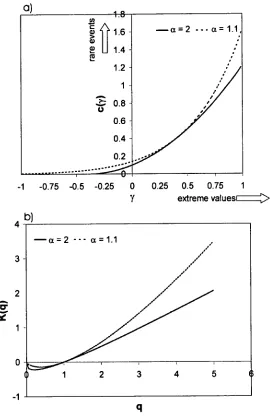
is a measure of the departure from conservation of the fluctuations of the

(30)

By varying these three independent parameters the FIF multifractal model can be used to describe or simulate a wide range of statistical behaviour. Examples of the functions c(7) and K(q) for several different parameter values are shown in Figure 2.2a and Figure 2.2b respectively. The parameter values appropriate for cloud fields are determined from aircraft measurements of cloud liquid water in Chapter 3.

2.1.4 'Bare' and 'dressed' quantities and multifractal phase

transitions

It must now be noted that the relationships for c("y) and K (q), described by (2.11) and (2.12) respectively, are only seen to hold in observed data up to some critical value of -y or q, above which the behaviour of these functions becomes linear [e.g.

Tessier et al., 1993; Chigirinskaya, 1994]. This behaviour at extreme 1, and q is known as Self Organised Criticality (SOC) and is described further in Schertzer and Lovejoy [1992] and Bak et al. [1987].

(31)

ra

re

eve

n

ts

—a= 2 - - a =1.1,

a)

IS: 0.8

0.6

0.4

0.2

-1 0 0.25 0.5 0.75 1

[image:31.556.144.414.169.586.2]

extreme values' >

Figure 2.2: Examples of the functions: a) c(7) and b) K (q) , for two values of a

and for C1 = 0.4. Note that K (q) must pass through the origin and (1, 0), and that

(32)

same spatial statistics for low values of the exponents q (or 7), and for the univer- sality classes of the FIF model, these are described by (2.11) and (2.12). But while the bare quantities follow these relationships for all values of q (or 7), the dressed

.1.1q1c

quantities have a critical-order moment qD (and corresponding 7D = (TD)) above

which the functions K (q) are not well defined because the statistical moments di-verge [Schertzer et al., 1993]. For dressed quantities of dimension D, the critical value qD is given by:

K(qD) — (qD — 1)D. (2.13)

However, for any particular measurement with a finite number of sampled points, the maximum value of q (or 7) for which K(q) (or c(7)) is well defined may be less than qD and is determined by the number of samples as well as the

di-mension [Schertzer and Lovejoy, 1992]. In this case the critical order qs below which

the structure functions show the behaviour predicted by the FIF model (equation 2.12) is predicted to be [Tessier et al., 1993]:

/.1)

+

D

s

Via

=

C1 )

where the sampling dimension Ds is given by D, = log N,/ log As . Here A, is the

maximum scale ratio in the measurements (i.e. maximum length divided by length of smallest resolution) and Ns is the number of realisations measured. For example,

if the data set were 5 aircraft flights measuring cloud properties at resolution of 100m for a total path of 100km per flight, then Ns would be 5, A, would be 1000

(=100km/100m) giving D, = 0.23.

The maximum q below which measured values of the universal exponent K(q) are well defined is therefore the smaller of qD and qs. The value of qD represents a

(33)

while q, is determined by the number of realisations sampled - this indicates that once the value of q, exceeds qD then any further increase in the number of sam-ples studied will not enlarge the range of exponents for which information can be obtained.

So for dressed quantities such as integrated measurements, the function K (q) (and c(7)) does not conform to equation (2.12) when q > min(qp, q,), but is instead linear in q. This change in the behaviour of the statistics of a measured multifractal field at a critical exponent is labelled a "multifractal phase transition" [Schertzer et

al., 1993]. Examples will be seen in the statistics of in situ measurements of liquid water content that are examined in Chapter 3.

2.1.5 Double trace moment analysis

The method used in this work to determine the multifractal behaviour of cloud liquid water content is the Double Trace Moment (DTM) technique of Lavallee et

al. [1993]. This method is summarised below for a one dimensional data series, such as the liquid water content measured from aircraft-mounted instruments. It can be used to test scaling and universality, and determines the parameters of the FIF model.

(34)

and differences are taken between the adjacent points in the data series, since this approximates the effect of multiplying by the wavenumber k in Fourier space. This

will produce the correct results as long as H is less than 1. If the resolution of the

sensor is at scale A', then the "pseudo-flux", co y , at point x is given by

40A, (x)

=

IP(x

+

Axv) — p(x)I (2.14)

where AxA, is the distance between adjacent points at resolution A' (AxA, = Lmax /A'). The flux is then raised to a exponent, n

,

and integrated to give a field at a lower resolution A. This field is labelled the "71-flux" I-1,71) and is given by:

Hi

ll)

(Xi) = (2.15)

with x1+1 = xi + AxA , i = 1, 2, ...., A, and Ax), is the distance between adjacent

points at resolution A (ax,. =

L

max

/A).

The double trace moment of the field at the scale A is then found by raising H(x) to a second exponent (q), summing over

the entire range (i.e. summing over all x i) and then taking the ensemble average, i.e.

A

TrA (WI )q = (E[H(An)(Xi)]q) (2.16) e

with an independent second exponent, q, being used. This process is repeated for

various values of exponents

n

and q, and for a range of scales A (all lower resolutions

than A'). If the process modelled is scale invariant then [Tessier et al., 1994

TrA((plij )q pc AK(q,n)-(q-1) _(2.17)

where the double exponent K(q,n) has been introduced. When n

=

1 the usual

(35)

a universal (FIF) multifractal the following holds [Lavanee et al., 1993]:

K(q,n)

=

qaK(q). (2.18)

Therefore a graph of log K(q, n

)

versus log 7? for a range of values of n should produce a linear relationship, the slope of which is a. The intercept of the line is log K(q) and hence, with a known a, the parameter C1 can be found using equation (2.12). This can be done for various values of q to improve the accuracy of the parameter derivation.

It should be noted here that when considering dressed multifractal fields, such as measurements with resolution above the homogeneity scale, the double exponent K(q, n

)

is affected by undersampling problems at high values of q or 1). This means that like K(q), the double exponent has critical order values above which it is not well defined and observations will not follow the relation (2.18). This problem should occur when the value of max(qn, n) is greater than min(qs , qp), where qs and

qD are the critical exponents defined in the previous section. As long as only values

of n lower than this are considered, then the relation (2.18) holds and can be used to find the parameters a and C1.

With a and C1 estimated, the parameter

H

can then be found from the energy spectrum, E(k), defined by

E(k)

_{= (}

_I

"(

k)1

2 +

IX-

0

2 ) ,

(2.19)

(36)

exponent, )3, is related to the parameter

H

by [Lovejoy and Schertzer, 1995b]:

/3 = 1 — K(2) + 2H,

and hence substituting from equation (2.12) for K(2) and rearranging, the following expression for

H

is obtained:

H

= 3 -1 Ci (2" — 2)

2 2(a — 1) (2.20)

In this manner all three of the parameters of the FIF model can be estimated using this technique.

2.1.6 Numerical simulation of multifractal fields

In order to use multifractal clouds in radiative transfer calculations, a method of numerically generating FIF multifractal fields is required. The generation technique used here is the "continuous cascade" method developed by Pecknold et al. [1993],

and it is summarised below. In this method the Fourier space techniques are used to generate a multifractal field at any scale.

As described in section 2.1.1, a multifractal cloud liquid water field p A at scale A can be generated from the stationary (multifractal) flux field (p), using Fourier

filtering. The question is then how to generate a stationary multifractal field such as

cpx . To determine the stochastic generation process, first we consider the properties

of the multifractal field co A and then find a random generation process that produces fields with these properties.

(37)

section 2.1.2; scale invariance; the multiplicative nature of the cascade process, as was described by equation (2.1) and shown in Figure 2.1. Scale invariance and the multiplicative nature of the cascade combine to give the following relationship between the field values at the same point but at two different scales:

=

WAWA, (2.21)

where A and A' are two spatial scales, so that AA' is a third scale at higher resolution than either of the two. Equation (2.21) is a result of scale invariance - it is saying that zooming in from scale A to scale AA' is the same as going from the top scale (A = 1) to A'.

Since it is often easier to deal with additive properties than multiplicative ones, it is convenient to introduce the generators FA of the multifractal field

(pA

such that

at each point

cloA =

exp(rA). (2.22)

Determining the generators FA is then sufficient to find the field (p A - so the goal is

now to find generators F A that satisfy all the known properties of the multifractal field. The multiplicative property of the field, (2.21), becomes an additive property of the generators so that

F

AA

, = FA' +

FA (2.23)

If the field is normalised so that <

cp), >=

1 then the definition of the universal

exponent function K (q), given by equation (2.6), gives

(exP(grA)) = (

A) = ,)

K(q). (2.24)

(38)

gives

exp(KA (q)) = AK(q) =< exp(qFA) > . (2.25)

This means that the function K),(q) describes how the statistical moments vary with A and is the 2nd Laplace characteristic function of the generator FA i.e. the logarithm of the Laplace transform of the probability density [Schertzer and Love-joy, 1991]. From this it is possible to determine all the properties required for the generators

r),

and these are [Pecknold et al., 1993]:

1. The set of generators must be stable under addition so that equation (2.23) always holds, i.e. the random number distribution must be such that the addition of numbers drawn from the distribution produces the same distribu-tion.

2. In order to be certain that the structure functions are finite (and K(q) is well defined) the probability distribution of the generator must fall off faster than exponentially for positive

rA,

as can be shown from (2.24) [Schertzer

and Lovejoy, 1991].

3. From equation (2.25), the Fourier spectrum of FA must fall off as the inverse of the wavenumber k in order to obtain a K),(q) that scales as In A, and hence to produce a K(q) independent of A [Pecknold et al., 1993].

4. If A is the highest resolution then the generator field

rA

must be band limited to between [1, A], since there should be no variations in the field at resolutions higher than A.

(39)

So to determine the generators

r,

the problem is then: what type of random number distribution will fit these 5 criteria? Levy distributions are the only stable, attractive classes of random variables under addition [Feller, 1971], and hence the

only set of distributions that satisfy the first criterion. Levy variables are defined as the limits of the normalised sum of independent random vectors, i.e. a Levy variable S is

X1 + X2 ± Xn

S

71-400 ni/C( (2.26)

where xi are independent random variables in R, and a is the Levy parameter (0 < < 2). To satisfy the second condition listed above we must choose only an extrema' asymmetric Levy distribution for the generators, that is one that has sig-nificantly more large negative values than large positive values, so that (epl) is finite for all q after exponentiation of the generators. A random value from an extrema'

Levy distribution can be calculated using the following expression [Chambers et al.,

1976]:

sina.(1)-400)

S(a) = (cos cl))1/a _{_ 4,) tan (1)}₊w

(r-W7r co2r ))

a1

a = 1 (2.27)

where (Do =- ( 1- 1 1 — al )/a, 41 is a random value drawn from a uniform distribution on (—I, I), and W is a random value drawn from an exponential distribution (Pr(W) = e-w). The random deviates 4:0 and W are mutually independent.

So to satisfy the first two criteria the asymmetric Levy variables are used. Using the relation (2.27) a single independent value S(a) is randomly generated from the

Levy distribution for each point in the field at the finest scale A. To obtain the correct statistics for the multifractal field, as given by (2.11) and (2.12), each of the variables S(a,x) is multiplied by ( 10 1/a [ Wilson et al., 1991]. The conditions 3

(40)

is to apply a fast Fourier transform (FFT) to the field of random Levy variables. The lc' behaviour of the Fourier spectrum demanded by condition 3 is achieved by multiplying the resulting Fourier spectrum by 'kr [Pecknold et al., 1993], where d is the number of dimensions of the field being generated. The fourth condition is

satisfied by filtering out any of the spectrum outside of the desired range of [1, A], i.e. multiply by the function f

(k,

A) which is 1 for lki < A and decays exponentially

for lki > A. The exponential decay is used instead of a sharp cutoff to zero because sharp cutoffs cause sinusoidal 'ringing' effects when transformed back to real space. Finally the difference between the FFT and the continuous Fourier transform is taken into account by multiplying by the following factor [Pecicnold et al., 1993]

k-ddk isd(A) 17,A •

ka

This gives a final expression for the field of generators of

(2.28)

)1/-

rA

= ((

c

_{a —}

1

1 S(a, k) IkI f (k, A) tcd(A)) (2.29) where ,§(a, k) is the Fourier transform of the field of random Levy variables, and

(41)

4

-

a)

30

25

20

(p 15

10 -

5

0

b) 100

90 80 70 60

(p 50

40

30

20

10

C 1 =0.8

C1 =0.4

C 1 =0.0E

o

50 100 150

X

200 250 300

50 100 150 200 X

[image:41.557.133.396.180.563.2]

250 300

(42)

0 50 100 150 200 250 3.5

3 -

2.5

2

1.5

1

0.5 -

—

X

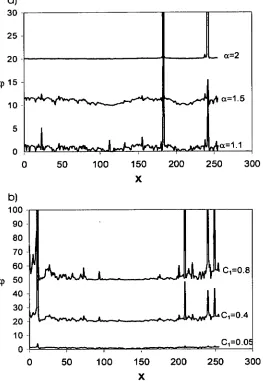
the field and the multifractal parameter a are the same quantity, i.e. multifractals generated using this method have a multifractica,lity parameter a equal to the Levy parameter used in their generation.

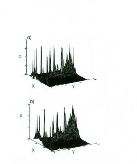
[image:42.557.136.413.264.468.2]

Generating the non-stationary field

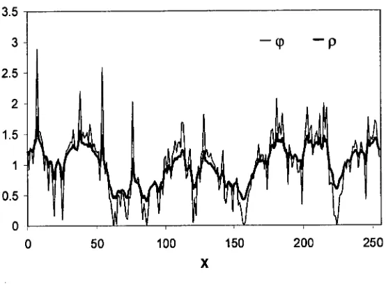
Figure 2.4: A numerically generated flux (pA in one-dimension, and the field PA that results from fractionally integrating the flux with

H =

0.3. Both fields are normalised so that the mean is one. Parameters are a = 1.5, C1

-=

0.1 and A = 256.

(43)

(1)

[image:43.556.82.524.67.596.2]

p

Figure 2.5: Examples of 2d multifracta1 generation with scale A =

128,

a = 1.5, C1 = 0.1. a) shows the flux field cp and b) shows the fractionally integrated field

(44)

then taking the inverse transform, that is

P = -

7.-1

(4

3 (k)ikl

-H

) ,

(2.30)

where -0(k) is the Fourier transform of the field of random Levy variables, and T - ' is the inverse Fourier transform function. This is known as fractional integration because if

H

is a positive integer then the result is the same as integrating the

field

H

times. This process allows the liquid water content field to be simulated

at any scale A by fractionally integrating the flux field, yoA, numerically generated as described above. The final step in generating the liquid water content field is to multiply

p

by the desired mean of the entire field (since the mean of the

field generated by the process so far is one). An example of the one dimensional simulated field

(pA

and the resulting PA are shown in Figure 2.4 for A = 256 and

H =

0.3. Note that the general effect of the fractional integration from

cp

A

to

PA is

a smoothing of the field. Figure 2.5 shows the same results for an example value of a two dimensional flux field (p A and the resulting PA with A = 256 and

H =

0.3.

It will be seen in section 3.2 that these simulated fields closely reflect the statistics of cloud liquid water.

A summary of all the steps taken in generating the multifractal liquid water content field is shown in flow diagram form in Figure 2.6.

2.2 Monte Carlo Radiative Transfer

(45)

ci))

Fourier transform

S (k, a) = F(S(

FA —

jig

-4 S

(k, ce)ild

cPA (X) =

exP(FA (x))

viv

Inverse transform

FA(x) = F

-1

(

1-

A(c)icd (A))

Generate S(x,a)

Ir

Fourier filter

F(VA)1Cd

This stage generates a random Levy variable at each point in the field at the highest resolution A, using equation 2.27. The variable x is the position, and a is the fractal parameter chosen for the field.

This stage takes a Fast FourierTransform FO, of the field S(x,a). The result is the field S(k,a), where k is the wavenumber

The Fourier transform of the generators TA is found by applying the power law factor Ikrdkt. , where d is the no. of dimensions of the field, and the normalisation factor cl

a - 1 )

The inverse Fourier Transform F- is then applied to the field, with the factor xd being a correction for the use of a FFT rather than a continuous Fourier transform, as given by equation 2.28

The stationary multifractal field yA is then found by taking the exponent of the generator field rA

A non-stationary multifractal field is then found using a Fourier Filter of Ikl-H on the stationary field CpA, where H is the chosen non-stationarity parameter.

(46)

- a large number of photons are traced through the media in question as they are scattered or absorbed. The main drawback of the Monte Carlo method is the relatively large amount of computer time necessary to trace a statistically significant number of photons through the system in order to get reasonably accurate results. A thorough description of the Monte Carlo method in radiative transfer and its various applications can be found in Marchuk et al. [1980]. In this section the basic technique used throughout this study to determine cloud radiative properties is outlined.

In this work the forward simulation method is used. This means that the pho-tons are traced from the time they enter the system until they leave or are absorbed, as opposed to a backwards Monte Carlo method where photons are traced in re-verse out from a fixed detector until they reach a light source. In this case the system in question is either a column of the atmosphere containing a cloudy layer, or simply the cloudy region alone. Both will be used later in this thesis, when the exact geometries used for different applications will be specified.

2.2.1 Photon tracing

(47)

used to trace each photon through the system:

1. The free path length 1 that the photon travels before the next collision is

determined (see section 2.2.2).

2. The possibility of the photon leaving the system is considered. If the photon encounters the top or bottom of the system before travelling a distance 1, the

current weight W is added to the total of the photons leaving the system, and the simulation of this photon is finished. Exiting photons are binned by exit position, exit direction, total path length travelled and number of scattering events before leaving. The horizontal boundaries are considered periodic, so that if they are encountered the photon reappears at the opposite side of the system at the same height.

3. If the photon has not escaped, the position of the next collision are calculated using the transforms x —> x + al, y y + bl, z —> z + cl.

4. The chance of absorption is taken into account. The probability that the photon is scattered at a collision event is the single-scattering albedo, w, of

the medium, so the chance of absorption rather than scattering is (1 — w). The weighting, W, of the photon is reduced to Ww, and the remainder of the weight, W(1 — w), is added to the total absorption in the medium.

5. The direction of the photon after the collision is determined from the phase function of the scattering medium. The phase function, P(0), is the

probabil-ity densprobabil-ity of having a scattering angle 0 between the incoming direction and

(48)

PP of a photon being scattered between 0 and 0 is then

PP(0)= foe P(01)d01 (2.31)

A uniform random number is chosen on [0,1] and PPM is set to this number.

Equation (2.31) is then solved numerically to give the upper limit 0, the

scattering angle. The azimuth angle, 0, of the scattering is then randomly chosen from a uniform distribution on [0, 27r]. If p = cos 0 then the direction of the photon after the collision is found using the transforms:

a —> ap — (b sin 0 + ac cos 0) [(1 — p2) ÷ (1 — C2)} 112 (2.32)

b—> ap — (a sin 0 + bc cos 0) [(1 — p2) ÷ (1 — c2)1112 (2.33)

c --+ cp — (1 — c2) cos (/) [(1 — p2)

÷

(1 — c2)}1 1 2 (2.34)

6. With the new direction, position and weight, return to step 1.

(49)

2.2.2 Maximal Cross-section method for finding free-path

length

The only step not fully detailed in the previous section was the method of deter-mining the path length

1

of the photon before a collision occurs. If the radiance of a beam of radiation in a particular direction is initially 10 , then after a distance

1

the radiance in the beam is

i

/ = /0 exP(— Jo

Oext(x)dx).

(2.35)

where Oext (x) is the volume extinction coefficient in the medium at the position x and is defined as the rate of extinction of a beam of radiation per unit length (with units of m-1). The exponent in (2.35) is the optical depth T along this particular

path, that is

r=

_I

1

f3

est

(x)dx = —

ln —/

o /0 (2.36)

The optical depth is therefore dimensionless. The probability of a photon having a collision in distance

1

is then

PR = L.

The simplest way to randomly generate a free path length

1

for a particular photon is therefore to generate a random

PR

using a uniform distribution on (0, 1). This is then used to give a random value of T using the expression T = - in

PR.

The equation (2.36) is then solved for the

free path length

1.

However this method can be difficult, or at least very time consuming, if the function Oext is complicated, such as a multifractal field on a high spatial resolution grid. Even though the field

f3

ext

is known, to solve (2.36) for

1

in a multifractal field it is generally necessary to accumulate optical depth grid-square by grid-square, and then linearly interpolate in the last grid-square.

(50)

shak et al. [1995] and Marchuk et al. [1980]. This method involves transforming

the integral radiative transfer equation [Marshak et al., 1995]

it •

V/ +13ext (x)/(x, ft) = wfiest J/(x, ST)P(SZ • rndST (2.37)

where

gx, n)

is the radiance at position x and in direction 1, and P is the phase

function. The first term on the left of equation (2.37) is the gradient of the intensity field, the second term represents the extinction of the intensity already travelling in the direction

n,

and the term on the right of equation (2.37) is the scattering source function. Equation (2.37) can be manipulated to give

1IV/+0,,ax /(x, SZ) =i3„,ax rext(x) wP(11 • IT) + (1 t) 6(1— ST)] /(x, ST)da,

O

max Omax

(2.38) where Omax = MaXx Oext (x). Equation (2.38) can be interpreted as the radiative

transfer equation for a fictitious medium in which f3max is the constant extinction

coefficient throughout the medium, and the phase function at any point is a com-bination of:

• wP(11 • ST), which occurs with a probability of r3e

i

t(x)

(physical scattering)

• Oft — ST), which occurs with a probability of 1PeZ(x) . ("mathematical scattering")

The first part of this modified phase function represents the physical scattering. The second part is purely a mathematical construct since the photon always goes in the same direction after it "scatters", because the delta function, 6(11— ST), is only non-zero when ft = ST. The true path length 1 in the real medium is then found

(51)

of solving (2.36) for the path length since the extinction coefficient is constant) until a collision occurs in which there is physical scattering rather than "mathe-matical scattering". Which type of collision occurs is randomly determined by the probability rietl:.(x) of physical scattering.

In summary, the following steps are followed to find the path length

1

in the

(real) medium:

1. Calculate the optical depth covered in the fictitious medium before scattering using T = — In

PR,

where

PR

is a random number from a uniform distribution

on (0,1).

2. The distance travelled is

l' =

Ti-Ana,„ since the fictitious medium has constant

volume extinction coefficient Omax .

3. Determine whether scattering at this point is physical or mathematical, using a uniform random number

R

between 0 and 1. If

R <

13 )

er

(x)

then the

scat-tering is physical, if

R >

)5

eit

(x)

then the scattering is purely mathematical

and the photon continues straight ahead.

4. If the scattering is purely mathematical then return to step 1 and repeat the process, if the scattering is physical then the process stops and the path length in the real medium

1

is the sum of the values of

l'

since the last physical

scattering.

This value of

1

is then used in the Monte Carlo algorithm described in the previous section (i.e. section 2.2.1). The advantage of this method of calculating

1

(52)

calculations in homogeneous cloud fields, but it is much faster for radiative transfer in multifractal clouds at small grid sizes.

2.2.3 Cloud properties

While the cloud properties used in the Monte Carlo simulations throughout this study will vary, it is possible to make some general comments about them here. Throughout this work the inhomogeneity in clouds is assumed to be solely due to variations in the number density of cloud droplets, not in the size of cloud droplets. Therefore the liquid water content varies but the droplet size distribution is constant throughout the cloud. In terms of optical properties this means that the scattering phase function and single-scattering albedo are constant throughout the cloud but the volume extinction coefficient O ezt varies in space. Although in some cases completely homogeneous clouds will be used in calculations for the sake of comparison, more often the focus will be on clouds whose liquid water content is multifractal and generated as was described section 2.1.6. The exact geometry and dimensions of the clouds will be specified later as they vary with the different applications. The resolution of the multifractal cloud is generally 25 m, meaning that the cloud is generated in a grid of cubes that are 25 m x 25 m x 25 m. The scale parameter A will then be given by

_ MaX

25m (2.39)

(53)

clouds [Marshak et a/., 1998; Cahalan, 1989]. This mean free-path length in liquid water clouds varies with the cloud properties but is on the order of 50 m [Marshak

et al., 1998].

If the cloud liquid water content allocated to grid-cube by the multifracta1 gen-eration method is p, then it can be related to the optical properties in the following manner The cloud liquid water content (in units of gm -3 ) at any point is related to the droplet size distribution by

00 4 0

p = DN i -ren(r).dr,

Jo 3 (2.40)

where D is the density of water (in gm-3 ), N is the total droplet number concen-tration (units of m -3 ) and n(r) is the (normalised) probability of the droplet radius being between r and r + Ar, for infinitesimal Ar. On the other hand, the volume extinction coefficient is given by

1.00

Oext = N I _J_o Qextn(r).7rr2dr (2.41)

where the extinction efficiency factor Q ext is defined as the ratio between the ex-tinction cross-section of a particle and its geometric cross-section and is given by the Mie scattering formula for spherical droplets [e.g. Goody and Yung, 1989]. Combining the two relationships (2.40) and (2.41), it can be shown that

3

(2 P

Oext = _{4D ref}

f (2.42)

(54)

n(r)r2 dr, and ref f is the effective cloud droplet radius defined by:

r n(r)r3dr ref

fo" n(r)r2dr . (2.43)

For the UV and visible wavelengths where the droplet radius tends to be signifi-cantly larger than the wavelength, _Qtand therefore

Q is very close to 2

[Stephens,

1976]. For other wavelengths, the Mie scattering formulae can be used to find

Q

for the droplet radius distribution in question, as well as the other single-scattering properties such as the phase function and single-scattering albedo. However Hu and Stamnes [1993] demonstrated that the single scattering properties of clouds varied

with changing effective radius but did not vary much between different shaped ra-dius distributions with the same ref f. In the same work, parameterisations of some of these single scattering properties were developed as functions of ref f and

wave-length, and these are used here to find

Q

and other single scattering properties. Therefore if ref f is chosen, the multifractal liquid water content field can be used in (2.42) to give

Oext

for each grid-cube. Generally a value of approximately 10 pm will be taken, since this is typical for low level liquid water content clouds [Han et al., 1994], but this is varied in some cases.

Apart from )3,t , the other properties required for the Monte Carlo model are the single-scattering albedo w and the phase function P(0). The parameterisation

of Hu and Stamnes [1993] give the w and the asymmetry factor g for each ref I (at each wavelength). The asymmetry factor is defined in terms of the phase function:

g = P(0)cosOde, (2.44)

(55)

only and g = 0 represents perfectly isotropic scattering. For visible wavelengths

and typical ref f values the asymmetry factor of liquid water clouds is approximately

0.85, indicating strong forward scattering. With the known asymmetry factor, the Henyey-Greenstein phase function PHG(0,g) is used in the Monte Carlo radiative

transfer - it is given by

1

-

PHG(0, 9) = (1 _g₂_-_{2g cos 0)}₃_/_2. (2.45)

This phase function, as opposed to a phase function constructed from the Mie scattering theory and typical droplet size distribution, was chosen in order to allow the phase function to be easily varied to test the effect of changing scattering properties on cloud radiative transfer.

Therefore a known liquid water field p and a chosen reff can be used to calculate

all the optical properties required for the Monte Carlo radiative transfer simulations. In this manner the multifractal model of cloud liquid water content and the Monte Carlo radiative transfer model are combined to determine the solar radiation field in clouds.

2.2.4 Whole atmosphere calculations

If we are performing radiation calculations for the whole atmosphere rather than just the cloud, as is done in section 6.2, the scattering properties neeii to be adjusted for non-cloud attenuation, such as Rayleigh scattering, aerosol or molecular absorp-tion (see Goody and Young [1989], Paltridge and Platt [1976], or Chandrasekhar

(56)

function in each grid square is then the weighted average of the phase functions,

with the weighting for each species being given by the value of fl ext for that species.

Similarly, the single-scattering albedo for each grid-square is the weighted average

over all the species, with each value of w being weighted by the value of O ert for

that species. Finally, surface reflectance can be taken into account by including the

chance of the photons being reflected from the lower surface of the system (instead

of passing out of the system), with the probability of reflection being given by the

(57)

Chapter 3 Analysis of in situ measurements

of liquid water content

3.1 Introduction

(58)

et al,

1997;

Davis et al.,

1994] to two other types of low-level liquid water clouds -

altostratus and low-level cumulus clouds. In this case there are two key questions: are they also scale invariant over a range of scales, and if so how do their fractal parameters compare to stratocumulus. In the case of stratocumulus cloud, not only are a significant number of flights added here to increase the data set analysed (over land in this case rather than in purely marine conditions) but an attempt is made to investigate the variability of the multifractal properties over time - both the diurnal and seasonal variations are considered.

To achieve these objectives, this chapter is structured in the following way. Ini-tially, some of the statistics of the liquid water field are presented for all three cloud types (stratocumulus, altostratus and cumulus) and the cloud fields are shown to be scale invariant. Subsequently, the data is compared to the FIF universal multifrac-tal model and the associated multifracmultifrac-tal parameters are empirically determined. The diurnal and seasonal variation in stratocumulus spatial structure is then in-vestigated. In addition, once the spatial distribution of the cloud fields has been parameterised, a relationship is found between mean liquid water content and the percentage of the horizontal layer filled with cloud.

Multifractal modelling of liquid water clouds : cloud spatial structure and its effect on the solar radiation field