Analysis of data to develop models for spray combustion

(1)

University of Southern Queensland

Faculty of Engineering & Surveying

Analysis of Data to Develop Models for Spray

Combustion

A dissertation submitted by

Jason Clarke

in ful…lment of the requirements of

ENG4112 Research Project

towards the degree of

Bachelor of Mechanical Engineering

(2)

Abstract

The design of modern petrol engines has placed an emphasis on lean combustion in

order to increase e¢ ciency, reduce operating noise and reduce pollutants. However,

the closer the engine operates to the lean combustion limit the higher the possibility

of engine mis…res occurring. Mis…res occur when there is not su¢ cient droplet density

around the spark to allow the evaporation of the droplets and hence the release of fuel

to the system.

The advent of injection systems has enabled engineers to control the majority of the

parameters of spray combustion, such as droplet size, droplet density and spray pattern.

Therefore, the ability to model spray combustion would have wide ranging implications

on the automotive industry.

One model which lends itself to the modelling of spray combustion is the Conditional

Moment Closure (CMC) model. However, the behaviour of the terms of the CMC

model, namely the conditional scalar dissipation, conditional source term and the

mix-ture fraction probability density function (pdf), is not understood well for this case.

A number of Direct Numerical Simulations (DNS) have been performed on di¤erent

cases of combustion where fuel droplets are present in cold air and a spark is used to

evaporate the droplets and initiate a ‡ame kernel. Data was collected and models were

developed for the three key terms of the CMC model.

Validation of the …rst order CMC model was performed by attempting to recreate

the behaviour of the DNS data. The performance of the …rst order CMC model was

(3)

conditional mean of the quantities. Another conditioning variable, or second-order

con-ditional modelling, may be needed in order for the CMC model to adequately capture

(4)

University of Southern Queensland Faculty of Engineering and Surveying

ENG4111/2 Research Project

Limitations of Use

The Council of the University of Southern Queensland, its Faculty of Engineering and

Surveying, and the sta¤ of the University of Southern Queensland, do not accept any

responsibility for the truth, accuracy or completeness of material contained within or

associated with this dissertation.

Persons using all or any part of this material do so at their own risk, and not at the

risk of the Council of the University of Southern Queensland, its Faculty of Engineering

and Surveying or the sta¤ of the University of Southern Queensland.

This dissertation reports an educational exercise and has no purpose or validity beyond

this exercise. The sole purpose of the course pair entitled “Research Project” is to

contribute to the overall education within the student’s chosen degree program. This

document, the associated hardware, software, drawings, and other material set out in

the associated appendices should not be used for any other purpose: if they are so used,

it is entirely at the risk of the user.

Prof F Bullen

Dean

(5)

Certi…cation

I certify that the ideas, designs and experimental work, results, analyses and conclusions

set out in this dissertation are entirely my own e¤ort, except where otherwise indicated

and acknowledged.

I further certify that the work is original and has not been previously submitted for

assessment in any other course or institution, except where speci…cally stated.

Student Name:

Student Number:

_____________________________ (signature)

(6)

Acknowledgments

This project was supervised by Dr. Andrew Wandel. I would like to thank him for his

support and technical expertise without which I could not have completed this project.

I would also like to thank my family for their continuing support.

Jason Clarke

University of Southern Queensland

(7)

List of Figures

1.1 Flowchart showing the coupling of CMC and CFD. . . 13

2.1 DNS results for the maximum temperature within the domain for …ve cases of equivalence ratio with droplet diameter constant. . . 27

2.2 Maximum temperature across the domain with a constant equivalence ratio and varying droplet diameter. . . 29

2.3 Conditional temperature over the life of the combustion. . . 31

2.4 Conditional mass fraction of fuel, all zones. . . 32

2.5 Conditional mass fraction of oxidiser, all zones. . . 33

2.6 Average mass fraction of fuel and oxidiser with respect to time. . . 35

2.7 Conditional variance between the species mass fractions. . . 36

2.8 Mixture fraction pdf, all zones. . . 37

2.9 Conditional scalar dissipation, all zones. . . 38

2.10 Conditional generation due to droplet evaporation, all zones. . . 39

(12)

LIST OF FIGURES xi

2.12 Behaviour of the conditional scalar dissipation for each zone. . . 46

2.13 Fit for the conditional scalar dissipation, zone 0. . . 47

2.14 Conditional scalar dissipation, zone 1. Note the transient behaviour. . . 48

2.15 Position of the local maxima with respect to time. . . 49

2.16 Position of the local minima with respect to time. . . 51

2.17 Conditional scalar dissipation, zone 1. Resultant …ts up to the local minima. . . 52

2.18 Resultant …t for the conditional scalar dissipation, zone 1. . . 53

2.19 Conditional scalar dissipation, zone 2. . . 54

2.20 Fit for the zone 2 conditional scalar dissipation until the local minima. . 55

2.21 Fits obtained for the tail of the zone 2 curves. These …ts have not been characterised. . . 55

2.22 Coe¢ cients of the cubic splines shown in …gure 2.21. The …t for coe¢ -cientdis shown as the dashed line. . . 56

2.23 Fit for the tail of the curves using coe¢ cients shown in equation 2.14. Note the inability to accurately predict the location of the minima. . . . 57

2.24 The …nal …t for the conditional scalar dissipation, zone 2, after the cubic splines are forced through the local minima. . . 58

2.25 Fit obtained for the conditional scalar dissipation, zone 3. . . 58

2.26 Conditional generation due to droplet evaporation, all zones. . . 59

2.27 Fit of the conditional generation, zone 0. . . 60

(13)

LIST OF FIGURES xii

2.29 Linear coe¢ cients in the form y=M(x c). . . 62

2.30 Fit for the conditional generation, zones 1–3. . . 63

2.31 Favre averaged mixture fraction for each of the zones with their

respec-tive …ts, case 2. . . 65

2.32 Fits for the conditional scalar dissipation, all zones, case 2. Fits for the

tail are omitted. . . 68

2.33 Fit for the conditional generation, zones 1–3, case 2. . . 70

3.1 Flowchart showing the steps taken when calculating the required

quan-tities using the CMC model. . . 74

3.2 Conditional temperature calculated by the …rst order CMC model (dashed

line) versus the the DNS data (solid line) over one quarter of the life of

the simulation. . . 80

3.3 A plot of …gure 3.2, zoomed in. . . 81

3.4 Conditional temperature calculated by the …rst order CMC model versus

the the DNS data over the life of the simulation. . . 82

3.5 Conditional mass fraction of fuel calculated by the …rst order CMC model

versus the the DNS data over one quarter of the life of the simulation. . 83

3.6 Conditional mass fraction of fuel calculated by the …rst order CMC model

versus the the DNS data over the life of the simulation. . . 84

3.7 Conditional mass fraction of oxidiser calculated by the …rst order CMC

model versus the the DNS data over one quarter of the life of the

simu-lation. . . 85

3.8 Conditional mass fraction of oxidiser calculated by the …rst order CMC

(14)

LIST OF FIGURES xiii

3.9 Variance of the conditional temperature as calculated from DNS data

and the mean conditional temperature calculated from the CMC model. 87

3.10 Variance of the conditional mass fraction of fuel as calculated from DNS

(15)

Chapter 1

Introduction

1.1

Introduction

Increasingly, governments and social pressure have required cars, and therefore engines,

to become more e¢ cient and produce less pollutants. Both Australian and American

governments have pledged to commit to reducing emissions from cars (Gillard (current

August 2010) and Crawley (current May 2010)). Beyond reducing emissions, increased

e¢ ciency of cars also translates to bene…ts for the consumer, with reduced fuel

con-sumption and lower engine noise. For these reasons, both industry and academics have

committed large amounts of resources to increasing the e¢ ciency of cars, and perhaps

of more interest to this thesis, engines.

In the motor industry today, almost all petrol engines have adopted the use of injectors

to supply fuel to the combustion chamber. The use of injectors has allowed a much

greater ability to control the parameters of spark assisted spray ignition than

carbu-rettored engines. Some parameters which may be adjusted are droplet size, droplet

density, spray pattern, spark intensity and duration. The advent of fuel injection has

also meant that the mixing of fuel and oxygen now takes place in the combustion

chamber.

(16)

1.1 Introduction 2

For stoichiometric mixing, the air to fuel ratio (mair=mf uel) should be 14:7for octane

fuels. However, traditionally, the mixture has been ‘rich’, or an air to fuel ratio in

the range of 12:5 13:3 to reduce the chance of engine mis…res. This however leads to unwanted pollutants, such as HC, CO and NOx. In order to design engines which

operate as lean as possible, accurate models of combustion are needed. The focus of

this project is to progress the development and implementation of such models.

The modelling of spray combustion is complex and not thoroughly understood.

Mod-elling of gaseous phase combustion is simpler than droplet combustion because the fuel

is already present in the correct phase. In spray combustion, however, the droplets must

…rst be evaporated by an area of localised high temperature (which may be created by

the spark energy or compression of the gas), and must continue to be evaporated by

the ‡ame front in order to continue releasing fuel to the system (Wandel, Chakraborty

& Mastorakos 2009). The e¤ect of the evaporation of the droplets with respect to the

‡ow …eld and temperature must be accounted for when attempting to model two phase

combustion.

Currently, there are four main methods used for modelling turbulent reacting ‡ows,

such as spray combustion. These are numerical modelling (Direct Numerical

Simula-tions (DNS)), large eddy simulation (LES), turbulent combustion models such as the

Conditional Moment Closure (CMC) model and models implemented in

Computa-tional Fluid Dynamics (CFD) software. LES still requires development for gaseous

combustion. The main disadvantage of numerical modelling is that it is

computa-tionally expensive; currently the processing power of computers has not allowed the

modelling of spray ignition for volumes larger than the order of 1cm3_{. The main}

dis-advantage of CFD is that since little is known about the evaporation of droplets in two

phase combustion, models must be developed to incorporate into the CFD software.

The models for incorporation into CFD software could potentially be developed from

use of the CMC model.

There have been numerous studies into combustion using the CMC model, however

most of the studies have relied on numerical data directly obtained from the use of

DNS, rather than prede…ned models. Prede…ned models for use in CMC modelling

(17)

1.2 Background and theory 3

in the CMC equation in the presence of evaporation. The current study aims to

reduce the gap in knowledge by analysing 3-D DNS data to generate models for the

key coe¢ cients in the CMC transport equation so that large-scale modelling may be

performed for sprays.

The broad objectives of this project are:

Analyse data from numerical simulations performed by Wandel et al. (2009) to

characterise combustion for a small control volume (approximately1mm3) using the CMC model,

verify the models’accuracy by recreating the data the models were obtained from,

code the models into a CFD package to allow for a much larger scale of modelling

to take place, and

model combustion in a simple combustion chamber to investigate the e¤ects of

changing parameters of spark assisted spray combustion.

1.2

Background and theory

1.2.1 O¤er of the project

This project was o¤ered by the faculty under the guidance of Dr. Andrew Wandel.

Andrew has a keen interest in the use of CMC methods to characterise combustion.

This project is an extension of research conducted by Andrew, from which a large

amount of data has been generated. This data has been used in the published paper

Wandel et al. (2009), but all the necessary quantities needed to solve the CMC model

are also present in the data.

1.2.2 Importance of fuel e¢ ciency and low emissions

In recent years, there has been a widespread political and social push for car

(18)

of the speci…c fuel consumption of an automobile per kilometre travelled. Emissions

refer to the production of harmful pollutants, such as HC, CO and NOx. Generally,

fuel e¢ ciency and level of emissions are linked; an increase in fuel e¢ ciency results in

a decrease in the production of pollutants.

Increasing the fuel e¢ ciency of a vehicle has been, and continues to be, the focus

of much research (Taymaz, Cakir & Mimaroglu (2005) and Nabi (2010)). There are

many positives associated with increasing e¢ ciency. Among these are: reduced fuel

consumption (resulting in lower costs of running and longer range of the car), reduced

engine noise, and fewer pollutants. Commercially, the production of e¢ cient cars is of

great importance as the majority of consumers value fuel e¢ ciency when buying a new

car.

There are numerous methods of increasing the brake thermal e¢ ciency of a car. Brake

thermal e¢ ciency is a measure of the output power of a car converted from the energy

stored by the fuel, and takes into account the thermal e¢ ciency of the engine cycle, the

mechanical e¢ ciency and the chemical e¢ ciency. Thermal e¢ ciency may be increased

by increasing the e¢ ciency of the combustion cycles (typically Otto or Diesel cycle)

by increasing compression ratio or decreasing the heat loss from the combustion to the

cooling system. Mechanical e¢ ciency can be increased by reducing any mechanical

losses, such as friction. The chemical e¢ ciency can be increased by ensuring all fuel

that enters the combustion chamber is consumed by the combustion. The …ndings of

this project could lead to an increase in the chemical e¢ ciency of an engine, but the

…ndings could also ‡ow on to reducing mechanical losses.

1.2.3 Background on two phase systems

This project focuses on spark assisted spray combustion, which is found in fuel injected

petrol engines. The presence of two phases (namely fuel in liquid, or droplet form, and

air in gaseous form) presents quite a problem when trying to model combustion. In

fact, the interaction of two phases without combustion is a complex phenomena and

has been the focus of many studies (Bini & Jones (2008) and Lebas, Menard, Beau,

(19)

There are many di¢ culties associated with trying to predict the behaviour of two-phase

mixing. Among these are: the e¤ect of turbulence on the mixing rate, the evaporation

of the liquid phase, droplet breakdown and the tendency of the droplets to coalesce.

These phenomena also prove to be computationally complex.

These problems are ampli…ed somewhat with the mixing occurring concurrently with

combustion. For combustion to take place, energy in the form of a spark must be

added to the system. This also has the e¤ect of evaporating fuel droplets and releasing

fuel to the system. The presence of fuel and oxidiser in gaseous phase, along with

heat from the spark, allows a ‡ame kernel to develop. Once the ‡ame kernel has

grown to a su¢ cient size and heat to stabilise, the spark may be removed. The ‡ame

kernel advances throughout the rest of the combustion chamber, …rst evaporating any

droplets nearby, and then consuming them in the combustion. Several factors in‡uence

the ability of the ‡ame kernel to proceed throughout the combustion chamber. If the

droplet size is too big, too little fuel is evaporated to allow combustion to proceed.

Likewise, if the droplet spacing is too big, fuel may become too sparse. If the spark is

removed prematurely, the ‡ame kernel may not be hot enough to become self sustained.

The ability to model two-phase combustion systems would allow the investigation of

the parameters which would encourage the most e¢ cient combustion.

When trying to model two-phase systems, the required outputs are most often the

mass fractions of each species, and temperature across the domain. The mass fractions

of each species are hard to model, because the rate of reaction between the fuel and

the oxidiser are highly non-linear functions of the mass fractions of fuel and oxidiser,

and the local temperature (Klimenko & Bilger 1999). Further complexity arises from

turbulence in the combustion chamber. This causes areas of highly di¤ering rates

of mixing and therefore the spatial location of combustion in the domain is largely

unpredictable. Also contributing to the di¢ culty of modelling spray combustion in

comparison to single phase systems is that some energy (in the form of a spray or

advancing ‡ame front) is needed to evaporate droplets and thus release fuel to the

system.

Due to the complexity of attempting to model two-phase systems, and in particular

(20)

approach is performing a DNS.

1.2.4 Direct Numerical Simulation (DNS)

DNS is a method of solving the Navier-Stokes equations numerically to describe ‡uid

‡ow. In a similar fashion to CFD, a given control volume is meshed (divided up into

a number of nodes) and the de…ning equations are solved at these points. However,

given that the Navier-Stokes equations are solved directly and without the use of

pre-de…ned models, the grid size must be much smaller than that used in CFD software.

For example Wandel et al. (2009) performed a DNS with a control volume with 1283

nodes. The control volume was cubic with length1:675mm. This equates to approxi-mately1:31 10 5_{m between adjacent nodes. The simulation, performed on a recent,}

commercially available computer, took a period of days to solve.

The computational time required for DNS is further increased when a chemical reaction

(such as combustion) occurs. While there has been some research into reducing the

computing requirements of the chemical reaction of n-heptane fuels (Lu, Law, Yoo &

Chen 2009), performing DNS on combustion any larger than the order of 1cm3 is too computationally demanding. While there has been widespread use of DNS to model the

behaviour of certain systems (Wang & Rutland (2007) and Sreedhara & Huh (2007)),

and it is a useful tool for verifying the results of other less demanding models, DNS

is of little use when modelling large scale systems, such as spray ignition. Therefore,

other methods of modelling large scale systems are needed. One of these methods is

the CMC model.

One of the advantages of using DNS is the ability to record vast amounts of data relating

to the combustion. This data, if analysed properly, can allow for a very thorough

understanding of the behaviour of the combustion. The data may also used to develop

(21)

1.2.5 Conditional Moment Closure model

The CMC model is used for the prediction of turbulent reacting ‡ows. Combustion

may be considered a turbulent reacting ‡ow as the burning of fuel and oxidiser is a

chemical reaction. The main advantage of the CMC model over DNS is that because it

uses prede…ned models, rather than solving the Navier-Stokes equations and reaction

equations directly, it is much less computationally intense and therefore can be used to

model much larger systems.

At the core of the theory behind the CMC model is that fundamental quantities of

combustion, such as species mass fractions, enthalpy and temperature, is conditional

on the mixture fraction (or ‘is a function of’the mixture fraction) (Klimenko & Bilger

1999). The mixture fraction is de…ned as the proportion of the mixture that was

originally fuel. The general form of the …rst order CMC model for homogenous cases

is:

@_hY _jZ_i

@t =hNjZi

@2_hY _jZ_i

@Z2 +hWjZi+hSjZi (1.1)

where:

The angle brackets denote the quantity to the left of the vertical bar is conditional

upon the quantity to the right (is the average of the left given a particular value

of the right),

Z =mixture fraction, or proportion of the mixture that was originally fuel,

hY _jZ_i = mass fraction of fuel or oxidiser,

hN_jZ_i=conditional scalar dissipation (equivalent to viscosity),

hW_jZ_i=conditional chemical source term (gain/loss due to chemical reactions),

hS_jZ_i=conditional generation due to droplet evaporation.

For stoichiometric combustion of n-heptane (as analysed in this project), the mean

(22)

The scalar dissipation, chemical source and generation due to droplet evaporation are

all quantities which must be modelled. The models for these terms may be derived

from DNS data, experimental data or analytical equations. One of the aims of this

project is to develop models for these three terms by analysing DNS data generated as

a by-product of the work undertaken in Wandel et al. (2009).

The CMC model is versatile due to its ability to be used for many di¤erent forms of

combustion, as well as the ability to predict many quantities such as mass fraction of fuel

and oxidiser, temperature and enthalpy. Depending on the nature of the combustion,

the form of the CMC model may change (Klimenko & Bilger 1999).

One of the main advantages of using the CMC model is that the quantities do not

need to be modelled with respect to their spatial coordinates, rather the quantities are

only conditional upon the mixture fraction. By reducing the number of independent

variables, the time necessary to model a system using CMC methods is dramatically

less than if DNS were to be used. For example, in the work performed as part of this

project, the time saved when modelling an equivalent system using CMC over DNS

was an order of magnitude of approximately 17000.

Given that the calculated values, such as mass fractions and temperature, are

condi-tional upon the mixture fraction, the distribution of mixture fraction throughout the

domain needs to be known in order to calculate the average values of those quantities.

The average value of any of the quantities calculated with the CMC model is given by

hY _i=

Z 1

0 h

Y _jZ_iP(Z)dZ (1.2)

where P(Z) is the mixture fraction probability density function. Therefore, in order for the CMC model to be useful, and therefore for the ability to verify the CMC model

against other methods, the probability density function must also be known. While

some forms of the mixture fraction probability density function are given in literature

(Sreedhara & Huh 2007), it may also be determined when performing a DNS. Therefore,

as with other terms of the CMC equation such as scalar dissipation, the mixture fraction

(23)

1.2.6 Terms of the CMC model

There are three main terms of the CMC model which require modelling. These are

conditional scalar dissipation, conditional chemical source and conditional generation

due to droplet evaporation.

The mathematical equation de…ning the scalar dissipation is:

N =D(_rZ _rZ) (1.3)

whereD is the di¤usivity and Z is the mixture fraction. The conditional scalar dissi-pation is equivalent to viscosity. Scalar dissidissi-pation is typically high at large values of

mixture fraction, as combustion occurs in rich areas. The combustion releases fuel to

the surrounding air, causing large variations in mixture fraction, and therefore large

gradients of mixture fraction. This in turn causes the scalar dissipation to be large.

The conditional generation due to droplet evaporation is a term which refers to the

contribution of the evaporation of droplets into gaseous phase to the mass fraction

of fuel. As the droplets are evaporated from the high temperature caused by either

the spark or the ‡ame kernel, more fuel is released into the system in gaseous phase.

Therefore, more fuel is present which causes the mass fraction of fuel to increase.

The conditional generation due to droplet evaporation is greater in rich areas where

combustion is more likely to take place.

The chemical source term,_hW_jZ_ican be approximated by an Arrhenius equation and is a function of the mass fractions of fuel and air, and the temperature. Because the CMC

model solves for the mass fractions as well as temperature, _hW_jZ_i can be calculated as the combustion proceeds. The chemical source term used is di¤erent depending on

which quantity is being solved for.

The mixture fraction probability density function may also be determined from DNS

data. Because the mixture fraction can be determined at every node in the DNS, the

relative probability of each value of mixture fraction occurring within the domain can

(24)

1.2.7 Limitations and assumptions of the …rst order CMC model

The …rst order CMC model is useful under many circumstances for modelling

combus-tion. The equation presented above (1.1) is a …rst order CMC model because there

is only one conditioning variable, mixture fraction. However, in certain cases, two

conditioning variables may be needed to fully capture the behaviour of the combustion.

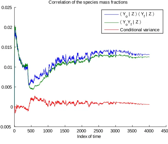
One of the assumptions implicit in the use of the …rst order CMC model is that the

conditional species mass fractions are strongly correlated, or

hY Y _jZ_i=_hY _jZ_{i h}Y _jZ_i+ Y00Y00_jZ (1.4) where the …nal term, DY00Y00_jZE or the conditional variance, is assumed to be neg-ligible. If the species mass fractions are strongly correlated, the conditional average

rate of reaction can be predicted using the conditional moments and the …nal term of

equation (1.4) may indeed be considered negligible.

In single phase systems, it has been found that under most circumstances that the

mass fractions of fuel and oxidiser are strongly correlated and as such the …rst order

CMC model accurately predicts the behaviour. In systems where local extinction and

re-ignition occurs, the mass fractions become less correlated and a higher order version

of the CMC equation is required. It is unclear whether the use of the …rst order CMC

model will accurately model two-phase combustion.

Single phase combustion which experiences local extinction and re-ignition has been

suc-cessfully modelled using a doubly-conditioned CMC model (Kronenburg & Papoutsakis

2005). Signi…cant variation in the values of mass fractions conditional upon mixture

fraction was found around the points at which extinction and re-ignition occurred. The

result of the high variance was that the …rst order CMC equation was unable to fully

predict the reaction rate at these critical points. In order to account for the signi…cant

variation about the mean, a second conditioning variable was introduced. This second

conditioning variable was sensible enthalpy.

There are two main factors which may in‡uence the ability of a …rst order CMC model to

accurately predict spark assisted spray combustion. It is unclear whether the presence

(25)

doubt that a …rst order CMC model will be able to account for signi…cant variations

in the mean occurring in areas adjacent the spark.

The use of a doubly-conditioned CMC model is beyond the scope of this project, but

the work presented here will be able to ascertain the validity or otherwise of the …rst

order CMC at modelling spark assisted spray combustion.

1.2.8 Objectives relating to DNS and CMC

This project will focus on characterising the terms of the single order CMC equation

presented in (1.1). The mixture fraction probability density function will also be

char-acterised. The data required to successfully create models for the CMC terms has been

recorded as outputs from a DNS performed by Wandel et al. (2009). DNS data is

available for several cases of combustion, which will be used to assess the adaptability

of the models created.

The …rst order CMC equation will then be solved numerically, and with the same

boundary and initial conditions as was used in the DNS. The quantities that will be

solved for are conditional temperature and the conditional mass fractions of fuel and

oxidiser. These values will then be checked against the values computed in the DNS.

The two main conclusions that are hoped to be drawn from this work are:

1. That all conditional quantities present in the single order CMC model can be

modelled accurately over the whole life of the combustion, and that these models

may easily be adapted for di¤erent cases of combustion.

2. To prove or disprove that the …rst order CMC model can be successfully applied

to spark assisted spray combustion.

If both of these objectives can be met, further work may focus on:

1. Using the models to predict the behaviour of much larger systems, either through

(26)

1.3 Literature review 12

2. If the …rst order CMC model is not su¢ cient, using the techniques presented in

this thesis to characterise the quantities of the CMC model with respect to two

conditioning variables as per the requirements of the doubly-conditioned CMC

model.

1.2.9 Application of the CMC model to CFD software

The CMC model could potentially be integrated into CFD software in order to model

large, dynamic systems. CFD software has the ability to accurately predict the ‡ow

…eld of a system, however currently the models used may not be suitable for spray

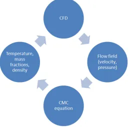
combustion. The ‡ow …eld refers to the velocity and pressure of the system.

Because the outputs obtained from CFD software (velocity, pressure) are inputs into the

CMC equation, and the outputs obtained from the CMC model (temperature, density)

are inputs into the CFD software, the two could be coupled in order to predict the

behaviour of large, dynamic combustion systems. The coupling of CFD and CMC can

be depicted graphically in …gure 1.1.

Each completion of the cycle is equivalent to one timestep. The integration of CMC

models into CFD software could potentially prove to be very valuable, more so with the

increasing computation power available. It could possibly be used to model combustion

in an engine or other large, complex systems.

1.3

Literature review

Literature published on the modelling of turbulent combustion of two phase systems

has been restricted to the last 15 years as the processing power required to perform

numerical simulations has become available. Most literature concerning DNS and CMC

models for spray combustion is published by two bodies, the Combustion Institute and

Combustion and Flame journal. Currently, there is somewhat of a void in the area of

(27)

[image:27.612.194.452.113.367.2]

Figure 1.1: Flowchart showing the coupling of CMC and CFD.

The CMC model and its uses

The most de…nitive article on the subject is Klimenko & Bilger (1999), “Conditional

moment closure for turbulent combustion”. This article aims to review all of the

pre-ceding knowledge of the application of the CMC model to “turbulent reacting ‡ows,

with particular emphasis on combustion”.

The article provides a comprehensive overview of the methods of developing

approxi-mations of the mixture fraction probability density function (pdf) for use in the CMC

model. A combination of , and Gaussian functions is used to model the pdf.

How-ever, this information is not needed in this project as data necessary to model the

pdf forms part of the data collected from the DNS simulations and therefore will be

modelled as per the other quantities.

In this article, the proposed CMC equation is

@Q

dt +hvjZi rQ+

div( _Z_hv”Y”_jZ_iP(Z))

P(Z) _Z hNjZi

@2Q

(28)

where the second and third terms of the left hand side are, for the purposes of this

project, negligible. This equation is largely consistent with that presented in Mortensen

& Bilger (2009).

The work of Klimenko & Bilger (1999) highlights the main void in current literature;

applying models derived from DNS data to the CMC equation.

Mortensen & Bilger (2009) derive equations necessary for CMC modelling for single

phase systems, two phase systems and separated ‡ow systems, with an emphasis on

two phase ‡ows. The article succinctly outlines the di¢ culty of modelling two phase

systems: “Mainstream approaches to modelling gas phase chemistry in sprays usually

assume that it can be treated in much the same way as in single phase systems. Little

attention has been given to the possible e¤ects of strong mixture fraction variations in

the neighbourhood of the evaporating droplets on the chemistry in a turbulent spray

‡ame. Potentially, CMC has the advantage that it can handle complex chemistry and

such e¤ects of the …ne scales of the mixing.”

The CMC equation derived for two phase combustion is

@Q

@t = huijZi @Q

@xi

+_hN_jZ_i@

2_Q

@Z2 +hW jZi

1

h i Zp

@_{h i} _Zp_hu00_iY00_jZ_i @xi

+ Q1; Q (1 Z)

@Q dZ

h jZ_i

h i

1

h i Zp

@(1 Z) _Zp_hY00 00_jZ_i

@Z (1.6)

where the …rst, fourth and sixth terms on the right hand side can be considered

negligi-ble. HereQ is any conditional quantity such asYf,Yo,T andh(enthalpy) and certain

terms, such as_hW_jZ_i;are to be used in their correct form with respect to the quantity being solved for. The article suggests that experimental methods for resolving some of

these terms is likely to be unsuccessful and advocates the use of DNS to fully evaluate

all of the necessary terms.

In addition to the terms shown in the general form of the CMC, equation (1.1), the use

of this form of the CMC model requires the use of the termQ1; : This term relates to

(29)

if the temperature was being solved for, Q1; is the temperature of the droplets. As

with other terms of the CMC model, this term may be determined from DNS data.

Uses of doubly conditioned CMC modelling

The use of doubly conditioned CMC modelling is becoming better understood as cases

where the assumptions of …rst order CMC modelling is invalid are investigated. One

such case of combustion that is not accurately modelled with the …rst order CMC model

is combustion in which local extinction and reignition occurs. Doubly-conditioned

CMC modelling is more complex than …rst order CMC modelling (as is used in this

thesis) as quantities such as scalar dissipation are conditional upon two variables. Kim,

Huh & Bilger (2002) investigated the application of doubly-conditioned CMC modelling

to combustion with local extinction and reignition.

The main focus of the work in Kim et al. (2002) was to investigate the ability of the

doubly-conditioned CMC model to predict the reaction rates of hydrocarbon fuel. A

very simple two step mechanism was used as an approximation of the reaction of the

fuel and oxidiser. "Two step mechanism" refers to the number of reactions required

for the fuel to fully react with the oxidiser. For example, a two step mechanism results

in one intermediate species, with in turn reacts with the oxidiser to form the products.

The results of the singly and doubly conditioned CMC were compared with DNS results.

The quantities investigated were the species mass fractions (including the intermediate

species) and the reaction rates. It was found that the doubly-conditioned CMC model

accurately predicted the reaction rates and species mass fractions, regardless of the

presence of local extinction and reignition. The …rst order CMC model predicted the

behaviour of some, but not all, quantities.

Kronenburg & Papoutsakis (2005) also investigated the use of doubly-conditioned CMC

modelling to identify localised extinction and reignition of the ‡ame kernel. In this

re-port, the conditioning variables were mixture fraction and sensible enthalpy. Modelling

of local quenching and reignition make investigation of ‡ammability limits, ‡ame

(30)

A DNS was performed with parameters such that local extinction and reignition would

occur, and in some cases global extinction would occur. Terms such as scalar

dis-sipation, mass fractions, rate of evaporation and temperature from both the

singly-and doubly-conditioned CMC models were compared with the DNS data. In most

circumstances the doubly-conditioned CMC captured the behaviour of extinction and

reignition quite accurately while single order CMC had some trouble predicting

reigni-tion.

This article demonstrates some of the ‡aws associated with …rst order CMC modelling.

If behaviour occurs which causes a signi…cant variation of the singly conditioned

quan-tities about the mean, the addition of another conditioning variable is needed. While

the events which cause this behaviour (extinction and reigntion) are not present in the

DNS data which has been captured for this project, other events such as the addition

and removal of the spark and evaporation of droplets may have a similar e¤ect.

Uses of DNS

Wang & Rutland (2007) used solely DNS to study the ignition of turbulent n-heptane

jets. The a¤ect of changing two parameters, droplet radius and velocity, was

investi-gated. Important …ndings from the article were that evaporative cooling due to the

evaporation of the spray and turbulent mixing are both important phenomena which

a¤ect the ignition of the jet. This research di¤ers from that being investigated in this

project because this project has a focus on combustion chambers rather than jets.

Other types of combustion

Fairweather & Woolley (2004) attempt to verify the results obtained from combustion

of a turbulent, single phase hydrogen jet with experimental results. The form of the

CMC which was used was not disclosed. Two di¤erent turbulence closure methods were

used to determine which would produce the most accurate predictions.

(31)

CH4-air counter‡ow streams. The form of the CMC model used was

@Q

@t = huijZi @Q

@xi

+_hN_jZ_i@

2_Q

@Z2 +hW jZi 1

e P(Z)

@ @xi

( u00_iY00_jZ Pe(Z)) (1.7)

where the …rst and fourth terms of the right hand side are considered negligible. This

is the simplest form of the CMC model advocated in literature and will form the basis

for the preliminary investigation of the accuracy of the models derived from DNS data

in this report.

Some of the quantities that are predicted with the use of the CMC model are the

mean mixture fraction pro…le at several points axially along the jet, the conditional

mass fractions of the fuel and oxidiser, the conditional temperature and the mean

temperature axially along the jet. The model is deemed to be quite accurate in the

prediction of the above quantities, however the authors do have some reservations about

the ability of the model to predict the release of nitrous oxides.

While this article is of little use in the context of this project, it does serve to

demon-strate the ability of the CMC model to predict a variety of reactions. It also highlights

the relative ease of the prediction of single phase systems.

Speci…c terms of the CMC model

Sreedhara & Huh (2007) investigated the conditional statistics of spray combustion for

two dimensional control volumes, with an emphasis on two dimensional turbulence. A

two dimensional control volume of length 2 cm with 1922 grid points was used. The e¤ect of varying the Sauter Mean Radius (SMR), the level of turbulence and droplet

velocity was investigated. A -function pdf was proposed and validated for the mixture

fraction. A linear …t for the conditional evaporation rate was compared against the DNS

data.

While this article aims to demonstrate the e¤ect of di¤erent parameters on the

evapo-ration and combustion within the control volume, the results are of little value to the

current work for a number of reasons. Several source terms were investigated, but were

not conditional upon the mixture fraction as is required for use in the CMC model. The

(32)

factor which may a¤ect the validity of the results is how turbulence was de…ned within

two dimensions; two dimensional DNS requires the use of arti…cial turbulence whereas

turbulence is a three dimensional phenomenon. Furthermore, the results obtained in

their DNS di¤er from the results studied in this project as they solved an autoignition

problem.

Massebeuf, Bedat, Helie, Lauvergne, Simonin & Poinsot (2006) attempted to quantify

the conditional source term due to droplet evaporation and conditional scalar

dissipa-tion rate which appear in the mixture fracdissipa-tion variance equadissipa-tion (and hence predict

the mixture fraction in a turbulent, two phase combustion). Models were proposed

for these quantities. The work in the article is similar to that of this thesis; deriving

models for CMC quantities.

Coupling of CMC and CFD

The coupling of the CMC model and CFD software has been performed on

compres-sion ignition in diesel engines (Wright (2010) and De Paola, Mastorakos, Wright &

Boulouchos (2008)). There has yet to be an investigation of spark ignition using this

method.

Wright (2010) outlines the basic steps required for the coupling of CMC models and

CFD software, as well as verifying the process against some experimental data. A …rst

order CMC model was used, and the CFD software used was STAR-CD.

The coupling of the CMC model and CFD was similar to that shown in …gure 1.1. The

CFD software, given input parameters such as initial temperature, density, velocity,

mass fractions and velocity, solves for the ‡ow …eld. The CMC model then takes those

outputs (such as turbulence) as input parameters and solves for the conditional species

mass fractions, temperature and enthalpy. A -function approximation for the mixture

fraction pdf is assumed, and is used to return the averages of the calculated values back

to the CFD software. The process is then repeated.

The second part of the article compares the results of the simulation with experimental

(33)

ignition delay (the time required for the fuel to ignite under compression) and mean

pressure rise were the quantities which were compared. The results showed that the

use of CMC and CFD was able to capture some of the behaviour of the compression

ignition. The accuracy of the results may have been a¤ected by a number of factors.

The use of …rst order CMC may have had some e¤ect on the ability to predict the

spatial location of some of areas of ignition, and on other combustion phenomena such

as behaviour at physical boundaries and local extinction and reignition. Also, the initial

conditions of the system would have been approximated to some extent which may have

led to some error.

The work in De Paola et al. (2008) shows a much more thorough discussion of the results

of coupling CMC and CFD for the simulation of an autoignition system. A heavy duty

diesel engine, for which experimental and numerical analysis has been performed, was

chosen. A …rst order, three dimensional version of the CMC model was used.

Some of the challenges of the modelling of a complex physical system, such as the

combustion chamber of a diesel engine, are discussed. Amongst these di¢ culties are:

accurately predicting the initial ‡ow conditions as the air enters the combustion

cham-ber, and the subsequent injection of fuel through the injector; the e¤ect of turbulence

on combustion; the complex nature of the chemical reactions; and the e¤ects of the

physical boundaries such as the piston crown and cylinder walls. Some discussion of

how to overcome these di¢ culties is present.

Again, the CFD software used was STAR-CD. Due to symmetry, a segment representing

one eighth of the combustion chamber was modelled. The use of the combustion

cham-ber as the control volume led to the volume and shape of the control volume constantly

changing as the piston oscillates between Top Dead Centre and Bottom Dead Centre.

How this change in volume was accounted for by the CFD software was discussed. As

the piston moves to the bottom of the stroke, and the expansion chamber expands,

some of the expansion is accounted for by the expansion of the mesh. However, once

the grid length surpasses a certain pre-de…ned length, another horizontal layer of nodes

is added to the grid. The mesh is then stretched again until another layer of nodes is

needed. The result of this is that at TDC there were 3680 cells and at BDC, 26945

(34)

1.4 Consequential E¤ects 20

The grid for the CMC model was di¤erent to that of the CFD grid. A pre-de…ned,

structured physical grid which encompassed the whole of the CFD mesh (the largest

of which occurs at BDC) was overlaid onto the CFD mesh. An algorithm was used to

determine which of the CMC cells were located within the control volume at any time,

and which were located outside of the control volume. The cells outside of the control

volume were discarded. The cells located within the control volume were coupled with

their corresponding CFD cells. The form of the CMC equation which accounts for

physical boundaries was used for cells located on the boundary.

The main method of validating the simulation against experimental data was the mean

pressure versus crank angle. The use of CMC coupled with CFD managed to accurately

predict the peak pressure which occurs slightly after TDC. The increase in pressure is

due to the combustion.

While the focus of the literature presented above is often quite narrow and tends to focus

on speci…c behaviour of di¤erent types of combustion, the methods used to calculate

results is often similar to that which will be used in this report. As the CMC model

lends itself to the simulation of many di¤erent types of combustion, it is envisaged

that the work completed in this report will have broad implications towards further

modelling some of the phenomena described above.

1.4

Consequential E¤ects

It is envisaged that this project will positively impact the engineering community, in

both the academic and industrial …elds. In the academic …eld, it will provide a

pro-gression towards more accurately modelling spray combustion using the CMC model.

In the automotive industry, it may be used as a design tool.

In the academic …eld, there is signi…cant e¤ort currently being put into developing

accu-rate models for spray combustion, as per the articles discussed in the literature review.

The analysis of DNS data to propose models for use in CMC would o¤er researchers

another avenue of predicting the terms of the CMC model, which are currently limited.

(35)

when trying to model certain phenomena or systems.

A greater understanding of spray combustion could lead to the application of the CMC

model to other systems. Some systems that are currently being investigated in literature

are jets, internal combustion engines and the combustion of counter-‡ow streams.

By applying the CMC model to CFD software, it would allow much more large-scale

modelling of real world combustion. This o¤ers the advantage of being able to model

the large scale systems before they are tested experimentally (in a similar fashion to

the modelling of ‡uid ‡ow over a wing before being tested in a wind tunnel).

In relation to industry, it is hoped that this project may prove to be a successful design

tool. The design of injectors could be improved by designing for a spray which gives the

best combustion. Three parameters that could be tweaked using the proposed model

would be droplet size, droplet density and spray pattern. The spark size and location

could also be incorporated.

There are also many articles which focus on improving injector design for the most e¢

-cient design. One article of interest is Reynolds & Evans (2003), “Improving emissions

and performance characteristics of lean burn natural gas engines through partial

strat-i…cation”. The ever increasing research and implementation of strati…ed-charge spark

and compression ignition is of particular signi…cance to the work being undertaken in

this project.

Strati…cation refers to the process of concentrating the injected fuel about the spark

while having the rest of the combustion chamber lean. The resulting air to fuel ratio

averaged over the whole of the chamber is lean, which cannot be achieved with regular

homogenous charge spark ignition. In the process of combustion, the spark ignites the

rich region of air-fuel mixture adjacent to the spark plug, which forms a stable ‡ame

kernel. This then propagates throughout the lean areas of the combustion chamber.

There are two main advantages of using full or partial strati…cation. These are increased

e¢ ciency at light loads and reduced emissions.

The use of strati…cation allows the use of much leaner mixtures than is currently possible

(36)

reducing the fuel injected into the chamber without throttling the air intake. The

pumping losses incurred by having to pump air through a constricted throttle can

a¤ect the e¢ ciency of the engine at low loads quite markedly, therefore varying the

engine output without using a throttle is advantageous.

The test system for the work in Reynolds & Evans (2003) consisted of a single cylinder,

naturally aspirated 4-stroke engine running on natural gas. In order to provide a portion

of the charge as a concentrated rich mass about the spark plug, a custom spark plug

injector was used. About 5 per cent of the mass of fuel was injected this way, giving a

partial strati…ed charge. The other fuel was injected using the existing injection system

and was lean. Using this system, they were about to achieve signi…cant (up to 7%)

reductions in the brake speci…c fuel consumption (a measure of fuel consumed per brake

power output).

The partial strati…cation system also o¤ers reduced levels of emissions, and in

partic-ular, reduced levels of NOx. The production of nitrous oxides is formed in the hot

exhaust gases before they leave the combustion chamber. One method of reducing the

formation of NOx is reducing the temperature of the exhaust gases. This is another

advantage of full or partial strati…cation; the temperature is high in close proximity

to the spark plug, but as the ‡ame front advances to the boundaries of the cylinder it

cools due to the sparse fuel. It was found that an optimum air to fuel ratio could be

found whereby HC and CO emissions were low (due to most of the fuel being burnt)

and NOx emissions were low (due to the cool outer region of the combustion chamber).

Ultimately, it was found that there was a limit to how much the engine output could

be controlled by controlling the air-to-fuel ratio (AFR). The mixture around the spark

had to be su¢ ciently rich to allow a ‡ame kernel to form, and the outer, homogenous

region had to be su¢ ciently rich to sustain the ‡ame kernel as it progressed towards

the cylinder wall. Using a mixture which was too lean would result in mis…res and a

reduction in e¢ ciency and increase in the release of HC and CO. The point at which

this starts occurring is called the ‘lean mis…re limit’.

Using the CMC model with data obtained from DNS would be a very suitable design

(37)

when a ‡ame kernel extinguishes, as well as the temperature in the combustion chamber.

This could lead to the design of more e¢ cient engines, and allow engineers to predict the

(38)

Chapter 2

Analysis of the DNS data

2.1

Overview of the DNS data

Wandel et al. (2009) performed DNS on a small, three dimensional control volume in

order to investigate the characteristics (droplet size and spacing) that would lead to full

combustion of a …ne mist of fuel. The fuel investigated was n-heptane. Navier-Stokes

equations were used to determine ‡uid movement. The control volume was a cube,

with 128 nodes along each edge, with the following characteristics:

Boundaries is the y- and z-directions were periodic (droplets which ‡ow out of the boundary re-enter through the opposite boundary).

Boundaries in the x-direction were “partially non-re‡ecting” (gradient at the boundary is zero, droplets do not re-enter).

Droplets were uniformly distributed throughout y and z co-ordinates, and be-tweenL=4 and 3L=4 in thex-direction.

The spark was centred in the control volume, and deposited energy for a

prede-termined period of time.

(39)

2.2 Selection of the DNS data 25

the duration of the combustion. This data is the basis for the …rst part of this thesis,

analysis of data to develop models for spray combustion.

There are three main regimes (“zones”) that may be observed in a successful burn when

a spark is turned on, then o¤:

Initial zone (<7 s): Little fuel vapour exists, combustion is almost non-existent, there is a rapid release of fuel to the system as the spark evaporates fuel.

Intermediate zone (7 165 s): The spark is either still on, or there is a strong

residual e¤ect from the spark and the droplet evaporation rate becomes

steady-state.

Final zone (>165 s): No residual e¤ect from the spark exists, droplet evapora-tion is steady-state for the remaining droplets (many are completely evaporated),

‡ame propagation is strong.

For the purposes of fully characterising the data, another stage was introduced. This

stage occurs before the initial stage, and for this very brief period, all quantities

ap-proximate the initial conditions before the spark begins evaporating fuel. This stage

will be referred to as zone 0.

2.2

Selection of the DNS data

There were eleven di¤erent sets of DNS data from which to choose. The combustion

di¤ered in two ways; the overall equivalence ratio and the droplet size. The equivalence

ratio, , is a ratio between the mass fraction of fuel that is supplied to the system

and the mass fraction of fuel required for stoichiometric burning. For example, an

equivalence ratio of two suggests that there is twice the amount of fuel present than is

needed for stoichiometric burning.

For the purposes of modelling the terms of the DNS data, a case in which combustion

(40)

point. In order to determine if the combustion indeed continued for the length of the

simulation, the maximum temperature in the domain was plotted versus time. The

maximum temperature was recorded when the DNS was performed.

2.2.1 The e¤ect of the equivalence ratio on combustion

As mentioned previously, in spark ignition systems, the equivalence ratio of the system

may greatly a¤ect the ability of the spark to form a stable ‡ame kernel. If the mixture

is too lean, not enough fuel will be evaporated for the ‡ame to consume. If the mixture

is too rich, not enough oxidiser may be present. Figure 2.1 shows the maximum

temper-ature in the domain over the length of the simulation for various values of equivalence

ratio. The initial diameter of the droplets is held almost constant in each case.

A normalised temperature equal to one refers to the adiabatic ‡ame temperature, or the

maximum temperature the combustion alone can sustain. The maximum temperature

may be greater than one due to the additional energy from the spark.

The graph for the equivalence ratio of 0.5 shows little or no combustion. The normalised

temperature is initially zero, indicating that no energy has been released to the system

yet. As time progresses, the temperature increases as the spark starts releasing energy.

At the peak of the curve, the spark is removed and the system gradually cools back to

its original state. The graph suggests that little or no combustion occurs, because it

seems that there is no other energy released to the system but the spark (the subsequent

graphs show a deviation upwards from the shape of the graph shown for = 0:5).

The maximum temperature shown in the case of equivalence ratio equal to one again

shows little combustion. There is some suggestion that there are small, localised areas

of burning (as evidenced by the slighter higher peak temperature than = 0:5), but these areas do not get su¢ ciently hot to produce a stable ‡ame kernel.

For the system with an equivalence ratio of = 1:5, a ‡ame kernel is formed and continues to burn until the normalised time is approximately0:275, at which point it extinguishes. This can be seen by the tail of the graph gradually returning to the initial

(41)

0 0.01 0.02 0.03 0.04 0.05 0.06 0.07 0.08 0

1 2

φ = 2.0

0 0.01 0.02 0.03 0.04 0.05 0.06 0.07 0.08 0

0.5 1 1.5

φ = 0.5

0 0.01 0.02 0.03 0.04 0.05 0.06 0.07 0.08 0

0.5 1 1.5

φ = 1.0

0 0.01 0.02 0.03 0.04 0.05 0.06 0.07 0.08 0

1 2

M

a

x

im

um

nor

m

al

is

ed

te

m

per

at

u

re

φ = 1.5

Maximum temperature vs. time

0 0.01 0.02 0.03 0.04 0.05 0.06 0.07 0.08 0

1 2

φ = 4.0

[image:41.612.180.468.182.613.2]

Normalised time

Figure 2.1: DNS results for the maximum temperature within the domain for …ve cases of

(42)

The graphs for = 2 and = 4 show that the ‡ame kernel becomes self su¢ cient and

does not extinguish before the end of the simulation. This can be seen by the maximum

temperature becoming steady at approximately 1.0 after the spark has been removed.

These graphs show the impact of the mass fractions of fuel and oxidiser on the

e¤ec-tiveness of the burn. If the system is too lean, the ‡ame is indeed extinguished as not

enough fuel vapour can be supplied. Of particular interest is the behaviour of

equiva-lence ratios1and1:5; while these mixtures were stoichiometric or rich, the combustion was still not e¤ective. This suggests that the droplet size may have been too great.

2.2.2 The e¤ect of droplet size on combustion

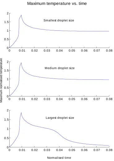
Figure 2.2 shows the maximum temperature for combustion with an equivalence ratio

of2 but with di¤ering droplet sizes.

The droplet sizes are:

Small: 2:783 m

Medium: 3:936 m

Large: 4:821 m.

It can be seen that for a given equivalence ratio, the droplet diameter may have an

e¤ect on the ability of combustion to proceed. In the case where = 2, the largest

droplet diameter cannot sustain the ‡ame kernel.

2.2.3 Selection of the DNS data

In order to characterise the terms of the CMC equation, a case of combustion which is

representative of most combustion will be selected. It is hoped that these models will

be readily adaptable to any other combustion, whether the air to fuel ratio, droplet

(43)

0 0.01 0.02 0.03 0.04 0.05 0.06 0.07 0.08 0

0.5 1 1.5 2

M

ax

im

um

norm

a

lis

ed

t

e

m

p

erat

u

re

M edium droplet size

0 0.01 0.02 0.03 0.04 0.05 0.06 0.07 0.08 0

0.5 1 1.5 2

Sm allest droplet size

Maximum temperature vs. time

0 0.01 0.02 0.03 0.04 0.05 0.06 0.07 0.08 0

0.5 1 1.5 2

Largest droplet size

[image:43.612.138.506.150.669.2]

Norm alised tim e

Figure 2.2: Maximum temperature across the domain with a constant equivalence ratio

(44)

2.3 Overview of important quantities 30

able to predict the behaviour of prematurely ending combustion up until the ‡ame is

extinguished.

The combustion which was chosen for initial analysis in this project is combustion with

an equivalence ratio of two and a droplet diameter of3:936 m:

2.3

Overview of important quantities

The three quantities that will be calculated using the CMC model are conditional

temperature and conditional mass fractions of both the fuel and the oxidiser. The

mixture fraction probability density function may then be used to …nd the mean values

of these quantities at any point in time. The following graphs show the data for each

of these quantities taken from the DNS. They give some insight on how the combustion

behaves.

2.3.1 Conditional temperature

Figure 2.3 shows a plot of the conditional normalised temperature over the life of

the combustion. The conditional temperature highlights the main values of mixture

fraction in which combustion is taking place. The stoichiometric mixture fraction in

this case isZ = 0:062. At low values of mixture fraction (and hence localised lean areas within the mixture), the temperature is low and almost equal to the initial temperature

before the spark was added. However, the temperature increases as the regime becomes

richer, and tends to peak and then plateau at high values of mixture fraction. This

suggests that combustion as expected is occurring in the rich areas while in the lean

areas no combustion occurs. Of particular interest is that combustion seems to occur

only at mixture fractions higher than stoichiometric. This agrees with the data shown

previously which suggested that of all the DNS data produced, only those simulations

with an equivalence ratio of two or higher could sustain combustion for the length of

the simulation. Given that most petrol engines today achieve consistent combustion

with mixture fractions approaching stoichiometric, it would suggest that the droplet

(45)

0 0.05 0.1 0.15 0.2 -0.2

0 0.2 0.4 0.6 0.8 1 1.2 1.4 1.6

Z

N

or

m

al

is

e

d T

e

m

p

e

ratur

e, T

Temperature vs. mixture fraction

[image:45.612.164.461.121.355.2]

Increasing time

Figure 2.3: Conditional temperature over the life of the combustion.

Recall that the conditional temperature is the mean of all the temperatures within the

domain given a particular value of mixture fraction. It was shown in …gure 2.2 that

the maximum temperature in the domain at all times is approximately equal to one,

which contrasts with the mean temperature shown in …gure 2.3 which is much lower.

This suggests that there is high variability of the conditional temperature.

Counter-intuitively, with increasing time, the conditional temperature decreases.

How-ever, the high temperature of the …rst curve occurs while the spark is still present. When

the spark is removed, the temperature decreases and stabilises. It also seems that as

time progresses, the ability of the combustion to occur in lean regions is reduced. This

is due to the reduced temperature of the ‡ame kernel with respect to the spark; the

high temperature of the spark is able to produce fuel more rapidly and thus in areas of

low droplet density is more likely to burn the fuel. Once the ‡ame kernel stabilises, it

(46)

0 0.05 0.1 0.15 0.2 0

0.02 0.04 0.06 0.08 0.1 0.12 0.14 0.16

Z

M

a

s

fr

a

c

ti

on

o

f f

u

e

l, Y

f

Mass fraction of fuel vs. mixture fraction

[image:46.612.159.462.120.354.2]

Increasing time

Figure 2.4: Conditional mass fraction of fuel, all zones.

2.3.2 Conditional mass fraction of fuel

Figure 2.4 shows the conditional mass fraction of fuel as the combustion proceeds. The

blue dots represent the initial mass fraction of fuel before the spark is added. The

oscillation at high values of Z is due to statistical error inherent in the process used to capture data from the DNS. In many ways, this graph rea¢ rms the inferences that

can be made from the graph of the conditional temperature.

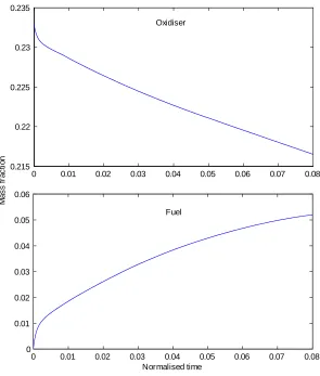
Initially, before combustion occurs, by de…nition the mass fraction of fuel is equal to the

mixture fraction. As combustion proceeds and the fuel is consumed due to it burning

in air, the mass fraction of fuel is reduced. Eventually, it is expected that most of the

fuel has been consumed and the mass fraction of fuel approaches zero.

As can be seen, the fuel is consumed in the rich regions of the domain, while the fuel

present in the lean areas is relatively untouched. This con…rms that combustion only

takes place in rich areas, and in this case the rate of combustio