Analysis and taxonomy of network quality of service (QoS) concepts in the long term evolution/system architecture evolution (LTE/SAE) System

(1)

iii

University of Southern Queensland

Faculty of Engineering and Surveying

Analysis and Taxonomy of Network Quality of

Service (QoS) Concepts in the Long Term

Evolution/System Architecture Evolution

(LTE/SAE) System

A dissertation Submitted by:

Saud Khlaif K Alenazi

In a fulfilment of requirements for:

Courses ENG4111/ENG4112

Toward the Degree of :

Bachelor of Engineering

(Electrical & Electronics Major)

Date of Submission:

(2)

iv

Abstract

Modern mobile communication networks provide a variety of voice and data services.

These services have different Quality of Service requirements and priorities. The

latest set of mobile technology specifications by the 3rd Generation Partnership

Project is referred to as Long Term Evolution/System Architecture Evolution. These

4th generation systems’ features major changes in access and core network as well as

service delivery. The main aim of this project is to investigate performance of the

Quality of Service concept of these systems. This includes an analysis of the

categorisation of the available Quality of Service mechanisms. In particular, the

project investigates and evaluates the performance features of the network. These

performance features include packets’ delay and downstream throughput. Better

performance of loaded network in the presence of Quality of Service mechanism is

one of the main goals of this project. More specifically, speed-up real-time packets as

they are the highest delay sensitive packets. Network simulator, NS2, is used to

emulate a LTE/SAE network and to simulate traffic. Simulation results show that the

throughput and delay of real-time packets are improved in the existence of Quality of

(3)

v

University of Southern Queensland

Faculty of Engineering and Surveying

ENG4111 & ENG4112

Research Project

Limitations of Use

The council of the University of Southern Queensland, its Faculty of Engineering and Surveying, and the staff of the University of Southern Queensland, do not accept any responsibility for the truth, accuracy or Completeness of material contained within or associated with this dissertation.

Persons using all or any part of this material do so at their own risk, and not at the risk of the Council of the University of Southern Queensland, its Faculty of Engineering and Surveying or the staff of the University of Southern Queensland.

The dissertation reports an educational exercise and has no purpose or validity beyond this exercise. The sole purpose of the course pair entitled “Research Project” is to contribute to the overall education within the student’s chosen degree program. This document, the associated hardware, software, drawings, and other material set out in the associated appendices should not be used for any other purpose: if they are so used, it is entirely at the risk of the user.

Prof. Frank Bullen Dean

(4)

vi

Certification

I certify that the ideas, designs and experimental work, results, analyses and conclusions set out in this dissertation are entirely my own effort, except where otherwise indicated and acknowledged. I further certify that the work is original and has not been previously submitted for assessment in any other course or institution, except where specifically stated.

Saud Alenazi

Student Identification Number:

0050077753

Signature:

(5)

vii

Acknowledgments

The author would like to acknowledge the efforts and assistance have been provided by the supervisor, Dr Alexander Kist. Dr Kist deserves thanks for continuous help and support throughout this project. Technical and Academic information have been provided by him, have guided the author to the right and proper way during the project.

(6)

viii

Table of Contents

Abstract ... iv

Limitation of Use...v

Certification...vi

Acknowledgement...vii

Table of Contents...viii

Table of Figures...xiii

Table of Codes...xvi

List of Tables...xvii

Chapter 1 : Introduction ... 1

1.1 Background ... 1

1.1.1 Mobile Systems Evolution ... 1

1.1.2 Long Term Evolution (LTE) ... 2

1.1.3 Long Term Evolution/System Architecture Evolution (LTE/SAE) ... 3

1.1.4 LTE Network QoS ... 4

1.2 Project Aim ... 4

1.3 Research Objectives ... 4

1.4 Dissertation Outline Overview ... 5

1.5 Chapter Summary ... 5

Chapter 2 : Literature Review ... 6

(7)

ix

2.1.1 Traffic Classes ... 6

2.1.2 Quality of Service Differentiation ... 7

2.1.3 LTE QoS Mechanism ... 8

2.2 Packet Scheduling ... 11

2.2.1 Packet Data Protocols ... 11

2.2.2 Packet Scheduling and Transport Channels ... 14

2.3 Throughput and Delay Calculation ... 21

Chapter 3 : Project Methodology and Simulation Model ... 23

3.1 Introduction ... 23

3.2 Network Simulator 2 (NS2) and LTE/SAE virtual network model ... 23

3.3 Network Model and Implementation ... 24

3.3.1 Flow Control ... 28

3.3.2 Network Configuration ... 28

3.3.3 Packet Classification and Scheduling ... 28

3.3.4 Traffic Model ... 29

3.4 Obtaining Results ... 35

3.4.1 Trace file ... 35

3.4.2 AWK Script File ... 36

3.4.3 Random Number Generator ... 40

(8)

x

3.6 Project Timelines ... 41

3.7 Conclusion ... 41

Chapter 4 : Test Scenarios and Simulation Results ... 42

4.2 Conversational Class Test Scenarios and Results ... 43

4.2.1 q0, Scenario 1 ... 43

4.2.2 q0, Scenario 1 Results ... 44

4.2.3 q0, Scenario 2 ... 46

4.2.5 q0, Scenario 3 ... 48

4.2.7 q0, Scenario 4 ... 50

4.3 Streaming Traffic Test Scenarios and Results ... 52

4.3.1 q1, Scenario 1 ... 52

4.3.3 q1, Scenario 2 ... 55

4.3.5 q1, Scenario 3 ... 57

(9)

xi

4.4 Interactive Traffic Test Scenarios and Results ... 61

4.4.1 q2, Scenario 1 ... 61

4.4.3 q2, Scenario 2 ... 63

4.4.5 q2, Scenario 3 ... 65

4.4.7 q2, Scenario 4 ... 67

4.5 Background (Best Effort) Traffic Test Scenarios and Results ... 68

4.5.1 q3, Scenario 1 ... 69

4.5.3 q3, Scenario 2 ... 71

4.5.5 q3, Scenario 3 ... 73

4.5.7 q3, Scenario 4 ... 75

(10)

xii

5.2 Assessment of Consequential Effects ... 79

5.2.1 Sustainability ... 79

5.2.2 Ethical Responsibility ... 79

5.2.3 Risk Management ... 80

5.2.4 Safety and Health Consequences ... 80

5.3 Resources ... 81

5.3.1 Sun Virtual Box ... 81

5.3.2 Ubuntu ... 82

5.3.3 Network Simulator 2 ... 82

Chapter 6 : Overall Summary and Conclusion ... 83

References ... 85

Appendixes ... 90

(11)

xiii

Table of Figures

Figure 1: Digital Communication Standards System (this figure made using MS office

power point) ... 2

Figure 2: Simplified LTE/SAE Network (this figure made using DIA software office power point) ... 3

Figure 3: Definition of QoS differentiation ... 7

Figure 4 : Architecture of LTE bearer service (3GPP TS 36.300) ... 8

Figure 5 : Typical packet protocols for real and non-real time services... 12

Figure 6 : Mapping of traffic classes to scheduling and to transport channels ... 12

Figure 7 : User Plane Protocol Stack ... 13

Figure 8 : Control Plane Protocol Stack ... 13

Figure 9: Principles of input information of cell packet scheduler ... 16

Figure 10 : DCH bit rate allocation ... 17

Figure 11 : the structure of RT and NRT Traffic packet scheduler in eNB (Jungsup Song et all, 2010) ... 19

Figure 12 : Interaction between P, LA &HARQ, in Frequency Domain (Pokhariyal et all, 2007) ... 19

Figure 13 : Mechanism used by the FD scheduler to allocate PRB resources to 1st transmission and retransmission users(Pokhariyal et all, 2007) ... 20

Figure 14 : Network Delay and Throughput Calculation ... 21

Figure 15 : Basic Architecture of Network Simulator (Issariyakul & Hossain, 2009 ) ... 24

(12)

xiv Figure 17 : LTE/SAE Network Model (this figure made using DIA software office

power point) ... 25

Figure 21: Queue classes (this figure made using MS office word and MS painter) .. 29

Figure 22 : RTP Traffic Travelled Initially from UEs ... 31

Figure 23 : RTP Traffic Arrives eNB coming from UEs ... 31

Figure 24 : All RTP Traffics enter the eNB ... 32

Figure 25 : RTP broadcasting ... 32

Figure 26 : Trace File Snapshot ... 35

Figure 27 : Project Tasks Timelines (this figure made using MS office Excel) ... 41

Figure 28 : q0 Received Throughput once q0 Traffic only Available ... 44

Figure 29 : q0 Delay once q0 Trafiic Only Available ... 44

Figure 30 : q0 Received Throughput once q1 UEs has increased ... 47

Figure 31 : q0 Delay once q1 UEs has increased ... 47

Figure 32 : q0 Received Throughput while q2 UE Increasing ... 49

Figure 33 : q0 Delay while q2 UEs Increasing ... 49

Figure 34 : q0 Received Throughput while q3 UEs increasing ... 51

Figure 35 : q0 Delay while q3 UEs Increasing ... 51

Figure 36 : q1 Received Throughput While Only Streaming Traffic is Available ... 53

Figure 37 : q1 Delay While Only Streaming Traffic is Available ... 54

Figure 38 : q1 Received Throughput while q0 UEs increases ... 55

Figure 39 : q1 Delay While q0 UEs increasing ... 56

(13)

xv

Figure 41 : q1 Delay While q2 UEs Increasing ... 58

Figure 42 : q1 Received Throughput while q3 UEs Increases ... 59

Figure 43 : q1 Delay while q3 UEs Increases ... 60

Figure 44 : q2 Received Throughput while Only Class2 Available ... 62

Figure 45 : q2 Received Throughput While q0 UEs Increases ... 63

Figure 47 : q2 Received Throughput while q1 User Equipment Increases ... 65

Figure 48 : q2 Delay while q1 User Equipment Increases ... 66

Figure 49 : q2 Received Throughput while q3 User Equipment Increases ... 68

Figure 50 : q3 Received Throughput, Only q3 Traffic Available ... 70

Figure 51 : q3 Delay, Only q3 Traffic Only ... 70

Figure 52 : q3 Received Throughput, while q0 User Equipments Increases ... 72

Figure 53 : q3 Delay, while q0 User Equipment Increases ... 72

(14)

xvi

Table of Codes

Code 1 : Setting Different Classes' User Equipments Number ... 26

Code 2 : Network Element Definition in tcl file ... 26

Code 3 : Node Connection Script ... 27

Code 4 : Real-time Traffic Simulation with aid of rtp protocol in tcl Code ... 30

Code 5 : Conversational Traffic codes ... 33

Code 6 : TCL Script Streaming Codes ... 33

Code 7 : Class3 codes ... 34

Code 8 : Trace File predifining code in main tcl file ... 36

Code 9 : AWK file Initialization 1 ... 36

Code 10 : AWK Script File Initialization2 ... 37

Code 11 : Throughput Calculation in AWK file ... 37

Code 12 : Delay Calculation Statements in AWK file for Classes 0, 1 and 3 Traffic . 38 Code 13 : Delay Calculation Scripts for Class2 Traffic ... 39

Code 14 : Commands to Run AWK Files in NS2 Terminal ... 39

(15)

xvii

List of Tables

Table 1: QoS Classes (Traffic Classes) ... 7

Table 2: QCI Standardisation ... 9

Table 3 : LTE and WiMax Contrast ... 10

Table 4 : Transport Channels Overview ... 15

Table 5: QoS Classes (Traffic Classes) and Simulation Protocol Used ... 30

(16)

1

Chapter 1 :

Introduction

In this project, a simple Long Term Evolution/System Architecture Evolution (LTE/SAE) model will be implemented and simulated in accordance with practical Quality of Service (QoS) parameters set by the operator and simplified for this project. Specifically, the total throughput, packet delay of this system will be tested when QoS parameters are enabled as well as when they are disabled. Long Term Evolution (LTE) is introduced to deal with the increase in the number of users and the need for high speed communications. It represents the fourth generation and most recent digital technology created since digital communication was invented. The Quality of Service (QoS) mechanism is essential to provide reasonable identification of the Long Term Evolution/System Architecture Evolution (LTE/SAE) System performance. Network Simulator 2 (NS2) tool is the nominated tool for building and testing the system. The expected results should show an improvement in the three tested criteria.

1.1 Background

1.1.1 Mobile Systems Evolution

(17)

[image:17.595.150.474.164.406.2]

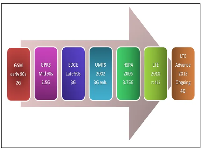
2 first decade of the 21st century. HSPA has improved the data bit rate to reach up to 14Mbps and it is known as 3.75 Generation. However, Long Term Evolution (LTE) is the major key that leads the communication technology to start the 4th Generation level.

Figure 1: Digital Communication Standards System (this figure made using MS office power point)

1.1.2 Long Term Evolution (LTE)

(18)

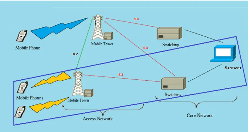
3 1.1.3 Long Term Evolution/System Architecture Evolution (LTE/SAE)

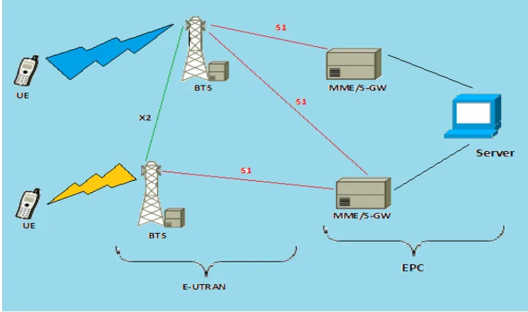
[image:18.595.142.513.486.705.2]

When these two terminologies, (LTE/SAE), come together, this results in LTE network architecture improvement. As a result, architecture complexity is eliminated due to reducing the number of nodes in the core network. Furthermore, the network becomes Flatter Network which means that the communication between stations in the network is performed without mediators such as routers. Therefore, the time taken for packets to travel is minimised which means latency is improved. Some of the nodes are redistributed in the network and/or merged to some other nodes since LTE/SAE elements have the ability to take place and substitute the user and/or control nodes. An example of this is the Radio Network Controller (RNC) that is split between the Access Gate Way (AGW) and Base Transceiver Station (BTS) or what is called (eNodeB). Core Network elements such as SGSN (Serving GPRS Support Node) and GGSN (Gateway GPRS Support Node) or PDSN (Packet Data Serving Node) are combine with the AGW. Figure 2 below shows simplified LTE/SAE network and it shows that the network includes two major parts, E-UTRAN (Evolved Universal Terrestrial Radio Access Network ) and EPC (Evolved Packet Core). UE is connected to the eNodeB via Air interface. The interface that connects the eNodeBs or BTSs together is the Air interface or x2 interface. Network nodes are connected to each other via S1 interface.

(19)

4 1.1.4 LTE Network QoS

When the service is shifted from single user to multi user service, the number of users is increased and higher traffic communication is needed. Therefore, it is important to define Quality of Service (QoS). QoS defines Policies rather than improving service’s features. QoS standardizations are in 3GPP release 8. A general example of QoS is when a supermarket has a policy which states that the customer should not wait for more than 1 minute at the checkout. The QoS in the LTE/SAE network is for both the access and service network.

1.2 Project Aim

The main aim of this project paper is to develop methods and techniques as well as providing measurements and test results analysis of the Long Term Evolution/System Architecture Evolution network environment in accordance to the Quality of Service concept. One more aim of this project is to provide an analysis of the categorisation of the available Quality of Service mechanism. In particular, the paper investigates the concept of bearer, evaluates the performance of the network as well as a number of applications and last but not least, aimed at being simulated in either real-time applications or mathematical model.

1.3 Research Objectives

Number of objectives has been set in order to achieve the main goals of the projects. The following dot points summarize the objectives:

• Researching the System Architecture Evolution/Long Term Evolution system

environment.

• Study and analyse of available Quality of Service mechanisms.

• Develop a mathematical models and/or simulation to evaluate the

performance of Long Term Evolution/System Architecture Evolution network.

(20)

5

1.4 Dissertation Outline Overview

This dissertation includes six chapters. Chapters’ titles and brief description of them are as following:

• Chapter 1: it is the introductory chapter, which includes: introduction,

background information of the project, project aim description, research objectives and dissertation outlines.

• Chapter 2: it is the Literature Review chapter, including a research on the

Quality of Service Mechanisms in regards to increasing the performance of system.

• Chapter 3: this chapter includes the project methodology and the simulation

model description.

• Chapter 4: it shows the test scenarios and simulation results concluded with

the discussion and analysis of results.

• Chapter 5: it includes the consequential effects and project resources.

• Chapter 6: this chapter summarizes and concludes the whole work has been

achieved in this project.

1.5 Chapter Summary

(21)

6

Chapter 2 :

Literature Review

This project covers a number of topic areas. Description of relevant subjects is introduced in this chapter. Literature includes Quality of Service and 3GPP traffic classes, packet scheduling techniques and investigation of throughput and delay calculation.

2.1 Quality of Service and 3GPP Traffic Classes

Long Term Evolution/System Architecture Evolution (LTE/SAE) network, has large variety of standardisations and requirements. These standardisations are made by different international organisations and operators of 3rd Generation of telecommunication technologies. This collaborated work is concluded with number of rules listed in documents. This collaboration project called 3rd Generation Partnership Project. 3GPP has number of releases; each one specific release has a start and end date. The recent updated release once this project has started is release 8. Release 8 has different number of versions. Parts of this release sections, concern of the requirements of network’s Quality of Service. The scope of this project is to look in details to the Quality of Service requirements in relation to traffic. Therefore, the following subsections discuss the traffic classes, quality of service differentiation and Long Term Evolution Quality of Service mechanism.

2.1.1 Traffic Classes

(22)

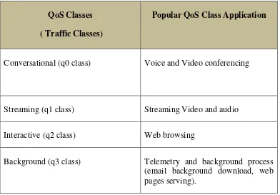
7 V8.0.0.Specifications. Table 1 below shows the four QoS classes and their popular

application.

QoS Classes

( Traffic Classes)

Popular QoS Class Application

Conversational (q0 class) Voice and Video conferencing

Streaming (q1 class) Streaming Video and audio

Interactive (q2 class) Web browsing

Background (q3 class) Telemetry and background process (email background download, web pages serving).

Table 1: QoS Classes (Traffic Classes)

2.1.2 Quality of Service Differentiation

[image:22.595.115.507.122.395.2]

Once the network is not loaded, the Quality of Service differentiation is not required. But once the network gets loaded, the QoS differentiation is highly recommended. The definition of QoS differentiation is depicted in Figure 3 below.

(23)

8 The real-time classes are the ones get benefits from the QoS differentiation, while the best effort classes are not much affected by the technique as they are low-delay service traffic. Ones the eNodeB node has the ability to identify different types of traffics; it can prioritise the traffic in relation to time sensitivity (Holma & Toskala 2007).

2.1.3 LTE QoS Mechanism

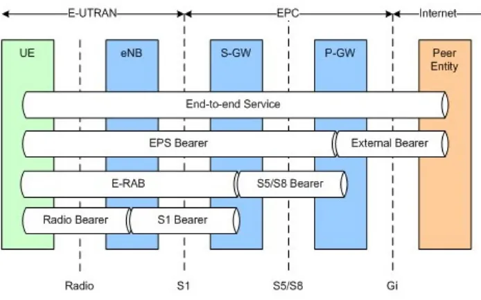
[image:23.595.137.484.469.686.2]

As it is defined in 3GPP TS 36.300, LTE/SAE Quality of service is a set of criteria and improvement parameters that have been defined to the network by the operator. These parameters would define the Maximum Bit Rate (MBR) which is the threshold value of the traffic rate, and they define the Guaranteed Bit Rate (GBR) value. QoS parameters and bearers are controlled by the signalling procedures in the Evolved Packet System (EPS), where the bearer is the mean of

i

dentifying the transfer and control of the stream of data packets and signals, which have been improved in accordance to QoS assigned for the network. The architecture of LTE bearer service is shown in Figure 4 below

(24)

9 Evolved Packet System (EPS) bearer is the stream of packets in between the user equipment (UE) and Packet Data Network Gateway (PDN-GW). Between each specific mobile equipment and service, there is a stream of data called Service Data Flows (SDFs). Evolved Packet System bearer/E-UTRAN Radio Access Bearer (EPS/E-RAB) is the indicator of bearer’s granularity in the radio access network. This means that a specific QoS treatment will be applied to all packets in same EPS bearer. An example of such treatment is a prioritisation scheduling. The Quality of Service Class Identifier (QCI) is to give an identity value to a specific bearer to identify the type of class included in this bearer. The QCI specifications are preset by network’s operator. Once the bearer has been firstly created, the GBR value would specify the type of resources that this bearer need. Services assigned to default bearers will experience Non Guaranteed Bit Rate (Non-GBR). It is standardized that the number of QCI values are unified due to roaming between networks. Table 2 below show this standardisation (Alcatel & Lucent 2009).

QCI Resource

Type Priority

Packet Delay

(ms)

Service Example

1

GBR

2 100 Conversational call

2 4 150 Live Streaming

3 3 50 Real-time gaming

4 5 300 Buffered streaming

5

Non-GBR

1 100 IMS Signalling

6 6 300 TCP-based buffered streaming

7 7 100 Interactive

8 8

300 Background

9 9

(25)

10 Once the call is firstly admitted to the network, it uses a parameter called Allocation and Retention Priority (ARP) to test if the nominated bearer is suitable to its type of traffic. Therefore, the main advantage of ARP parameter is to avoid any prospected risk results from the wrong assigned bearer. In layer two of the transport layers shown in Figure 4, the radio bearer is the stream of data used to transfer data in between the user equipment (UE) and eNodeB and it can be named as X1 bearer. S1 bearer is the stream of data in between eNodeB and Core Network (CN) which is used to transfer data between the Access Network (E-UTRAN) and Core Network (CN). In addition, S5 and S8 bearers are the bearers used in between Core Network elements (Alcatel & Lucent 2009).

According to Vadada (2009), to distinguish between the QoS service differentiation in LTE and QoS differentiation of WiMax, a comparison has been made in Table 3 below.

QoS Transport Unit

Scheduling

Types QoS Parameters

QoS Handling

in the Control

Plane

WiMax Service Flow UGS rtPS nrtPS BE

MSTR≠MRTR Network and user initiated control

LTE Bearer GBR

Non-GBR

GBR=MBR only network

initiated QoS control Table 3 : LTE and WiMax Contrast

The comparison made in Table 3 is generally divided in four items:

• QoS Transport Unit: the transport unit used in WiMax as specified in IEEE

802.16 is the Service flow which is the packets flow connecting the mobile station to base station while LTE uses bearer between the mobile phone and gateway.

• Scheduling Type: WiMax uses different type of schedulers, they are

(26)

11 service (nrtPS) for delay-tolerant traffic which need some rate to be reserved and Best effort (BE) service for usual services where LTE uses Guaranteed Bit Rate and non-Guaranteed Bit Rate bearers.

• Quality of Service parameters: WiMAx lets the operator to predefine traffic

prioritisation and Maximum Sustained Traffic Rate (MSTR) and Minimum Reserved Traffic Rate with different values while LTE state that the operator must set Guaranteed Bit Rate and Maximum Bit Rate at same values.

• Control Plane: in WiMax the network initiated control or the user initiated

control and network initiated control are both available while in LTE only network initiated control is available.

2.2 Packet Scheduling

This Section will discuss number of subsections. These subsections include packet data protocols, transport channels, and packet scheduling techniques have been investigated by number of researchers.

2.2.1 Packet Data Protocols

(27)

12 Figure 5 : Typical packet protocols for real and non-real time services.

The real-time traffics such that conversational and streaming traffic needs guaranteed bit rates where the non-real time traffics doesn’t need guaranteed bit rate. Conversational real-time traffic doesn’t need scheduling and it is transmitted over Dedicated Channel (DCH). Figure 6 below shows the mapping of traffic classes to scheduling and to transport channels.

Figure 6 : Mapping of traffic classes to scheduling and to transport channels

(28)

[image:28.595.128.465.72.275.2]

13 Figure 7 : User Plane Protocol Stack

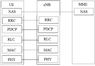
Packet Data Convergence Protocol (PDCP), Radio Link Control (RLC) and Medium Access Control (MAC) layers are terminated in eNodeB. The main functions behind the user plane are scheduling, ciphering, header compression, ARQ and HARQ. The control plane that controls the user plane is as shown in Figure 8 below.

[image:28.595.123.512.427.696.2]

(29)

14 The new layers introduced in Figure 8 are the Radio Resources Control (RRC) that terminated in eNodeB from the network side, and the Non-Access Stratum (NAS) that terminates at the MME from the network side. RRC main functions are radio resource management, scheduling, compression and decompression and many others.

2.2.2 Packet Scheduling and Transport Channels

The packet scheduler in LTE network is located in eNodeB. The air interface measurements is measured by the eNodeB itself and they are forwarded to the packet scheduler. In addition, the information of size of the upstream traffic is provided by user equipment (UE). This section includes the user packet scheduler description

2.2.2.1 Transport Channels for User Scheduler

. There are number of transport channels used in LTE network in regards to packet transfer. These transport channels and their relation to scheduling is discussed in the following subsection.

2.2.2.1.1Common Channel

Common Channels in LTE network are the Random Access Channel (RACH) as an uplink channel, where the downlink common transport channel is Forward Access Channel (FACH). These two channels are used as user data transport channels. The common channels can cause more interference than other channel types due to that they can use soft handover (Holma & Toskala 2009, pp. 271-2).

2.2.2.1.2Dedicated Channel (DCH)

(30)

15

2.2.2.1.3Downlink Shared Channel (DSCH)

This type of channels used for bursty packets transport. It is used with DCH in parallel, if DCH is a lower bit rate channel. It is not suitable in the case of soft handover. It is suitable for the slow start TCP. This channel can be assigned to another UE before the time located for DCH is up, due to this it is called shared channel (Holma & Toskala 2009, pp. 274-5).

Table 4 below shows the transport channels overview.

DCH DSCH FACH RACH

RRC state Cell_DCH Cell_DCH Cell_FACH Cell_FACH

UL/DL Both DL DL UL

Suited for Medium and large data size

Medium and large data size

Small data Small data

Suited for Bursty data

No Yes Yes Yes

Available in first network and terminal

Yes No Yes Yes

Table 4 : Transport Channels Overview (Modified from Holma & Toskala 2009, p. 274)

2.2.2.2 Cell Packet scheduler

(31)

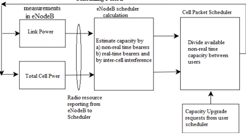
The cell packet scheduler needs number of inputs to do scheduling these inputs are as follow:

• The power value of eNodeB • The estimated load

• Bearers capacity in relation to throughput, especially non • Maximum interference level c

• Requests of bit rate need upgrade.

[image:31.595.126.525.313.534.2]

Figure 1 below shows the main principle of the input information and calculations needed by the cell packet schedule

Figure 9: Principles of input information of cell packet scheduler

2.2.2.2.1Priorities

The Quality of Service parameters are set by operator and it is provided to the EUTRAN network from core network (CN).

includes number of important information such that allocation retention priority and the network traffic classes.

radio resources between users efficiently.

The cell packet scheduler needs number of inputs to do scheduling these inputs are as follow:

The power value of eNodeB The estimated load

Bearers capacity in relation to throughput, especially non Maximum interference level can be tolerated

Requests of bit rate need upgrade.

below shows the main principle of the input information and calculations needed by the cell packet scheduler.

: Principles of input information of cell packet scheduler (Modified from Holma & Toskala 2009, p. 280

Priorities

The Quality of Service parameters are set by operator and it is provided to the EUTRAN network from core network (CN). The quality of service parameters number of important information such that allocation retention priority and ic classes. This information is provided to let eNodeB distribute the radio resources between users efficiently. From these parameters, the packet scheduler 16 The cell packet scheduler needs number of inputs to do scheduling efficiently, and

Bearers capacity in relation to throughput, especially non-real bearers

below shows the main principle of the input information and calculations

Modified from Holma & Toskala 2009, p. 280)

(32)

gets clear picture of how the capacity to be distributed. specified for high priority traffic will use the

low priority will hold until the previous bearer is executed. priority number is assigned to different traffic types.

(Falconio & Dini 2004

• Weighted Fair Queuing (WFQ):

In this strategy, the buffer with the highest number of data will be served first by the link.

• Early Deadline First(EDF):

After assigning a deadline to each packets are the once to be served first.

• Hybrid Algorithm

It is a mix between the WFQ and EDF, where the buffer length, arrival time of packets and the class each packets are belong to are known. The packet to b served is the ones with either highest length, or the lowest deadline figure.

2.2.2.2.2Scheduling Algorithm

In regards to the provided parameters, cell packet scheduler chooses the suitable bearer to every single type of incoming traffic.

[image:32.595.130.537.502.721.2]

below shows the DCH bit rate allocation.

Figure 10 : DCH bit rate allocation

gets clear picture of how the capacity to be distributed. The bearers that they are high priority traffic will use the available capacity while the bearers with low priority will hold until the previous bearer is executed.

priority number is assigned to different traffic types. In one of the relevant studies io & Dini 2004) Examples of prioritisation algorithm are as follow:

Weighted Fair Queuing (WFQ):

n this strategy, the buffer with the highest number of data will be served first Early Deadline First(EDF):

fter assigning a deadline to each packets in the buffer, the lowest deadline packets are the once to be served first.

Hybrid Algorithm:

t is a mix between the WFQ and EDF, where the buffer length, arrival time of packets and the class each packets are belong to are known. The packet to b served is the ones with either highest length, or the lowest deadline figure.

Scheduling Algorithm

In regards to the provided parameters, cell packet scheduler chooses the suitable bearer to every single type of incoming traffic. As an example of this

below shows the DCH bit rate allocation.

: DCH bit rate allocation

17 The bearers that they are capacity while the bearers with low priority will hold until the previous bearer is executed. Different allocation In one of the relevant studies Examples of prioritisation algorithm are as follow:

n this strategy, the buffer with the highest number of data will be served first

packets in the buffer, the lowest deadline

t is a mix between the WFQ and EDF, where the buffer length, arrival time of packets and the class each packets are belong to are known. The packet to be served is the ones with either highest length, or the lowest deadline figure.

(33)

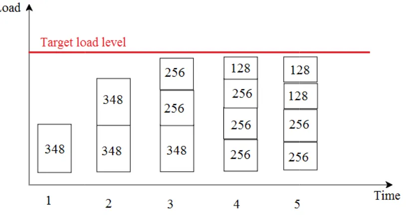
18 The capacity of cell is assumed as 900 kbps. The first user capacity will be 348 kbps; the second one will get the same value once we have only two UE. Once we have 3 users, it is not possible to have 348kbps, then the first one will maintain having 348kbps but the remaining two get 256kbps each and so forth. The downgrading operation represents the bearer bandwidth downgrade. The upgrade operation is permitted in the case that one of the bearers is free of use. This algorithm shows the distribution of resources once there is only one type of traffic classes’ available (Holma and Toskala 2009, p. 282).

Different scheduling schemes can be applied in eNodeB more specifically in Radio Resource Management (RRM) as operator needs. Some of them depend on the channel behaviour and link characteristic. Another Scheduling schemes are in regards to the Traffic Behaviour. At low load system, there is no significant difference between different scheduling schemes. This difference is highly significance in high load systems. One more factor will make the difference more significance is the behaviour of the Traffic. According to Holma & Toskala (2002), number of popular algorithms is discussed in the following three sub-sections.

2.2.2.2.3Fair Throughput Scheduling Algorithm

The scheduler receives information about the bit rate offered in the cell. This available bit rate will be distributed equally between the users. This algorithm can be used for real-time traffic as it can offer a guaranteed bit rate to the users.

2.2.2.2.4Fair Time Scheduling

In this scheduling scheme, all user equipments are assigned at same power. The throughput is distributed in regards to the channel condition. The user equipments enabled to use higher throughput are the user equipments with high channel quality.

2.2.2.2.5C/I Scheduling

(34)

19 Schedulers such as the latest three types, use Time Domain Packet Scheduler (TDPS) followed by Frequency Domain Packet Scheduler (FDPS) phases.

Figure 11 : the structure of RT and NRT Traffic packet scheduler in eNB ( Song et al, 2010)

Once we have more than one traffic class in a system, the classifier is important for the packet scheduling. Different queues with different priorities are set by the classifier for different traffic types. It can be seen from Figure 11 above that the classifier at layer 2 buffer assigning the each stream of one type of traffic with its class (Song et al, 2010). There are different Quality of Service requirements for each class.

The degree of fairness as it is discussed above is achieved with interaction between the HARQ and Packet Scheduler (PS). This interaction is depicted in Figure 12 below.

(35)

20 By looking at Figure 12, it shows the cooperation between the Packet Scheduler (PS), HARQ management and Link Adaptation (LA). These are existed in the eNodeB. Packet Scheduler is the controlling item. Physical Resource Block (PRB) is showing the resolution of the scheduling. In the frequency domain the bandwidth of PRB is 375 kHz minimum for one block and it is 24 PRBs in the 10MHz BW.

The Packet Scheduler will get a help from LA to know the data rate of different users having different PRBs. The Link Adaptation is highly dependent on the Channel Quality Indication (CQI). CQI helps LA as it obtain the users’ feedback. HARQ manager has information about the buffer (Pokhariyal et al 2007).

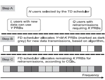
Time Domain (TD) scheduler will identify the number of users N in the highest priority to go to Frequency Domain (FD) Scheduler. TD considers the new data users and keeps in touch with the users with retransmission requests which are not prioritized by TD. FD scheduler’s function is to give M available number of the PRBs to N users. Figure 13 shows the HARQ management steps (Pokhariyal et all, 2007).

Figure 13 : Mechanism used by the FD scheduler to allocate PRB resources to 1st transmission and retransmission

[image:35.595.127.463.470.725.2]

(36)

2.3 Throughput and Delay

According to Oleg Berzin network is provided. T

calculated, the following network example is provided.

Figure 14 : Network Delay and Throughput Calculation

Number of elements and figures in di: is the delay of link where i=1,2,3....L Ri: Link bit rate, where i=1, 2, 3...L P: Number pf payload bit per packet H: number of Header bits per packet K: Number of packets per window

The general equations to find the sent packets’ delay is shown in equation 1 below

For the throughput calculation, it is simply found by dividing the bi taken to be transported.

Throughput and Delay Calculation

Oleg Berzin (2010), throughput and delay calculation method of network is provided. To understand how the packets delay and

calculated, the following network example is provided.

: Network Delay and Throughput Calculation

Number of elements and figures in Figure 14 are to be explained first. di: is the delay of link where i=1,2,3....L

Ri: Link bit rate, where i=1, 2, 3...L P: Number pf payload bit per packet H: number of Header bits per packet

mber of packets per window

∑

Equation 1

For the throughput calculation, it is simply found by dividing the bi taken to be transported.

21 throughput and delay calculation method of nd how the packets delay and throughput are

are to be explained first.

(37)

22 To find a specific link throughput is as follow:

( )

Equation 2

2.4 Chapter Summary

(38)

23

Chapter 3 :

Project Methodology and

Simulation Model

3.1 Introduction

The major goal of this project is to evaluate QoS features of the LTE/SAE network, and to build a model simulating this network. The network performance will be evaluated by analysing the throughput and delay while QoS parameters are enabled as well as when they are disabled. A comparison between the two situations triggered and non-triggered QoS features will be investigated. One more criterion to be examined is the packet flow of information being transmitted edge to edge from the eNodeB to the GateWay.

3.2 Network Simulator 2 (NS2) and LTE/SAE virtual network model

An initial step to complete this project is to be familiarized with the tools required for building a LTE/SAE virtual network. Background knowledge of the LTE/SAE system itself is a supportive factor to build a model. Network Simulator 2 (NS2) is the nominated software simulator to model the system and to obtain accurate results. It is industry approved software that is widely used by communication engineers for networking research. The LTE/SAE model will include the Network Model and Traffic Model. The Network Model includes the following interfaces Air interface and S1 interface. Separating these two models would increase the reusability and flexibility of the LTE/SAE model.

(39)

24 Figure 15 : Basic Architecture of Network Simulator (Issariyakul & Hossain, 2009 )

As it is illustrated in the above figure, the NS2 mainly consists of two main languages, C++ and Object-oriented Tool Command Language (OTcl). C++ in NS2 is mainly existed for simulation objects’ mechanism definition. The OTcl is used for simulation scheduling discrete events’ setting. The main simulation script as shown in the above figure is the very far left item. It is used to set up network topology, links, setting the type of traffic between nodes and much more input arguments. It is run via an executable command ns followed by the name of the script. The name of this project main simulation script is lte.tcl and it is provided in the appendixes. The first right hand item is the output information file, which can be used to obtain and graph the results.

3.3 Network Model and Implementation

LTE/SAE Model and its Implementation in NS2, is a project’s paper investigates Long Term Evolution network performance (Qiu et al, 2009). The results have been tabled in the paper were initially faulty. Starting from this paper, an improved project simulation model is made to test the performance of LTE/SAE network.

(40)

25 Figure 16 : The parts of LTE/SAE network to be simulated

[image:40.595.123.540.71.292.2]

In clearer picture, the LTE/SAE network model to be simulated is shown in Figure 17 below.

Figure 17 : LTE/SAE Network Model (this figure made using DIA software office power point)

The network model needs to be configured on demand therefore; number of elements and bandwidth parameters between them can be changed, added and/or eliminated. The only limitation to the model that is the eNodeB and Gateway which are permanent and fixed and cannot be moved or multiplied.

(41)

26 The following figures of codes show how the network model’s elements built in tcl file

set numberClass0 5 set numberClass1 2 set numberClass2 1 set numberClass3 1

set number [expr {$numberClass0 + $numberClass1 + $numberClass2 + $numberClass3}]

Code 1 : Setting Different Classes' User Equipments Number

The first four lines of the Code 1 above are to set the number of user equipments for each class, where the last line is the total number of user equipments in the network. The steps of defining network’s elements in the script file are demonstrated in Code 2 below

set eNB [$ns node];#this node id is 0 set aGW [$ns node];# this node id is 1 set server [$ns node];# this node id is 2 for { set i 0} {$i<$number} {incr i} {

set UE($i) [$ns node];# node(s) id is > 2 }

Code 2 : Network Element Definition in tcl file

Node 0 in the simulation stands for eNB, node1 refers to Access Gate Way, the Main Server’s number is 2 and any number greater than 2 refers to user equipments.

(42)

27

for { set i 0} {$i<$number} {incr i} {

$ns simplex-link $UE($i) $eNB 10Mb 2ms LTEQueue/ULAirQueue

$ns simplex-link $eNB $UE($i) 10Mb 2ms LTEQueue/DLAirQueue

}

$ns simplex-link $eNB $aGW 100Mb 2ms LTEQueue/ULS1Queue $ns simplex-link $aGW $eNB 100Mb 2ms LTEQueue/DLS1Queue .

$ns simplex-link $aGW $server 1000Mb 2ms DropTail $ns simplex-link $server $aGW 1000Mb 2ms DropTail

Code 3 : Node Connection Script

(43)

28 3.3.1 Flow Control

To avoid any packet loss due to downlink limitation, Flow Control is required. The flow control has been represented in the model with Air interface downlink Queue and S1 interface downlink Queue Script files. Air interface downlink Queue Script file provides the flow with the required information such as average data rate while S1 interface downlink Queue Script File decides whether or not to send the packet to the Air Interface down link queue in accordance to available information. The scripts of the flow control are written in C++ language and they are included in the appendixes.

3.3.2 Network Configuration

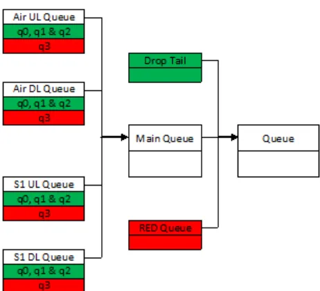
S1 and Air interfaces are to be simulated by setting and implementing queue classes in the network model. These Queue Classes are LTE main Queue, Air interface down link queue, S1 interface Uplink Queue, and S1 interface downlink Queue. In the main class, the condition of whether or not to use these optimization features are defined. Other classes define the interface implementation.

3.3.3 Packet Classification and Scheduling

(44)

[image:44.595.166.397.94.304.2]

29 Figure 18: Queue classes (this figure made using MS office word and MS painter)

3.3.4 Traffic Model

(45)

30 QoS Classes

( Traffic Classes)

Popular QoS Class Application

Simulation Protocol Used

Conversational (q0 class) Voice and Video conferencing Session/RTP

-Session/RTPAgent -Session/RTCPAgent

Streaming (q1 class) Streaming Video and audio CBR/UdpAgent

Interactive (q2 class) Web browsing HTTP/TcpAgent

- HTTP/Client - HTTP/Cache - HTTP/Server

Background (q3 class) Telemetry and background process (email background download, web pages serving).

[image:45.595.113.543.71.470.2]

- FTP/TcpAgent

Table 5: QoS Classes (Traffic Classes) and Simulation Protocol Used

3.3.4.1 Class0 Traffic Simulation

To simulate the conversational real-time traffic, it has been initially simulated by using rtp protocol as Code 4 : Real-time Traffic Simulation with aid of rtp protocol in tcl Code tcl coding below shows

for { set i 0} {$i<$number} {incr i} { set s0($i) [new Session/RTP]

set s1($i) [new Session/RTP] set group($i) [Node allocaddr]

$s0($i) session_bw 12.2kb/s $s1($i) session_bw 12.2kb/s $s0($i) attach-node $UE($i) $s1($i) attach-node $server }

(46)

31 After simulating real-time traffic, unpredicted results for the throughput are obtained where the sent traffic is much lower than the received packets without any packet drop. After observing the traffic by running NAM network animator in NS2, it shows that this traffic is a broadcasting traffic. The following figures will show the traffic animation has been observed.

Figure 19 : RTP Traffic Travelled Initially from UEs

Figure 19 above shows the RTP traffic once it is initially travelling from UEs towards the eNB. Nodes number 3,4 and 5 are the user equipments. Node0 is the eNB. Node 1 is the Access Gate way. And the node number 2 is the main server.

Figure 20 : RTP Traffic Arrives eNB coming from UEs

(47)

32 Figure 21 : All RTP Traffics enter the eNB

Figure 21 above shows the moment that all RTP traffic packets have entered the eNB node.

Figure 22 : RTP broadcasting

Figure 22 above shows the problem clearly where packets are broadcasting traffic, where they are broadcasted to all nodes at the same time, going to all user equipments as well as access gateway. This is not suitable for telephony service.

(48)

33 Code 5 below shows the part of script codes to create conversational traffic

for { set i 0} {$i<$numberClass0} {incr i} { set null($i) [new Agent/Null]

set nullS($i) [new Agent/Null] $ns attach-agent $UE($i) $null($i) $ns attach-agent $server $nullS($i)

set udp($i) [new Agent/UDP] set udpUE($i) [new Agent/UDP]

$ns attach-agent $server $udp($i) $ns attach-agent $UE($i) $udpUE($i)

$ns connect $null($i) $udp($i) $ns connect $nullS($i) $udpUE($i)

$udp($i) set class_ 0 $udpUE($i) set class_ 0

set cbr($i) [new Application/Traffic/CBR] set cbrS($i) [new Application/Traffic/CBR] $cbr($i) attach-agent $udp($i)

$cbrS($i) attach-agent $udpUE($i) $ns at 0.4 "$cbr($i) start"

$ns at 0.4 "$cbrS($i) start" $ns at 40.0 "$cbr($i) stop" $ns at 40.0 "$cbrS($i) stop" }

Code 5 : Conversational Traffic codes

The conversational traffic codes in Code 5 above shows that the traffic are set in both direction where the cbr over udp agent are set at the user equipment side which terminated at the server side, and for the other direction the cbr over udp agent is set at the side of server to simulate the conversational traffic travels from server and terminated at the side of user equipments.

3.3.4.2 Class 1 Traffic Simulation

for { set i $numberClass0} {$i<

($numberClass0+$numberClass1)} {incr i} { set null($i) [new Agent/Null]

$ns attach-agent $UE($i) $null($i) set udp($i) [new Agent/UDP]

$ns attach-agent $server $udp($i) $ns connect $null($i) $udp($i) $udp($i) set class_ 1

set cbr($i) [new Application/Traffic/CBR] $cbr($i) attach-agent $udp($i)

$ns at 0.4 "$cbr($i) start" $ns at 40.0 "$cbr($i) stop" }

(49)

34 While the streaming traffic comes from the server to the user equipments, the traffic agent and protocol to be set in the side of server and terminated at the side of user equipments where the null agent to be set. To avoid any misdistributions of the traffic over networks the number of user equipment must not set as numbers, but it must use a range distribution to avoid distributing more than one traffic type to the same user equipment. This is clearly shown in the first line of the Code 6 above where the first user equipment using class1 is equal to the last one who is using the class0 traffic plus 1. The number assigned to last user equipment to use class1 traffic is equal to number assigned to last user equipment using class0 plus the number of user equipment will use the class1 traffic.

3.3.4.3 Class2 Traffic Simulation

Over TCP Agent, class2 simulation is done by setting HTTP/Server at the side of main server, HTTP/cache at the side of access gateway and HTTP/client at the side of user equipment. The average page size each user can see is 10K. The script of creating this traffic type is attached in the appendixes.

3.3.4.4 Class3 Traffic Simulation

Over TCP agent, FTP protocol in the side of main server is set to simulate class3. This traffic sink at the side of user equipment. Code 7 below shows the script codes of creating class3 simulation.

{$i<($numberClass0+$numberClass1+$numberClass2+$numberCla ss3)} {incr i} {

set sink($i) [new Agent/TCPSink] $ns attach-agent $UE($i) $sink($i) set tcp($i) [new Agent/TCP]

$ns attach-agent $server $tcp($i) $ns connect $sink($i) $tcp($i) $tcp($i) set class_ 3

set ftp($i) [new Application/FTP] $ftp($i) attach-agent $tcp($i) $ns at 0.4 "$ftp($i) start" }

(50)

35

3.4 Obtaining Results

This section discusses the script files used to calculate the required results. This section includes number of subsections as follow, trace file, AWK script files, and Random Number Generator Set.

3.4.1 Trace file

In the tcl script file, predefining the trace file is important, due to that; all information of NS2 based simulation is included in the trace file. This file’s information sample is shown in the Figure 23 below which is a snapshot of one of trace files obtained in this project tests. The format of the trace file lines is shown in Table 6 below.

Figure 23 : Trace File Snapshot

The first symbols in the left hand side in each means as following: (r): Received packet

(+): enqueue (ــ): dequeue

(d): dropped packet

(51)

36 event time

Source Node

Dest. Node

Pkt Type

Pkt Size

Flags

Flow ID

Src Addr

Dest Addr

Seq Num

Pkt ID

Table 6 : Trace File Line Format

In the main tcl file, the trace file must be predefined and it is predefined in this project main tcl file as it appears in Code 8 below.

set f [open out.tr w]

$ns trace-all $f

Code 8 : Trace File predifining code in main tcl file

From this trace file, the simulation results are obtained by reading the file. The way it is followed in this project to obtain the results is by writing a script in an AWK file.

3.4.2 AWK Script File

Two awk script files are used in this project’s simulation to extract the results out from trace file and doing calculation on trace file’s information. The first awk script is to calculate the throughput received, sent and dropped of the first mobile equipment use specific class traffic. The second awk script is used to calculate the time delay of this mobile phone’s traffic.

3.4.2.1 AWK Script to Calculate Throughput

In the beginning of this script, number of initializations are to be set such that Code 9

BEGIN{

flag=0;

UEclass0=-1;

UEclass1=-1;

UEclass2=-1;

UEclass3=-1;

}

(52)

37 In this part of initialization, BEGIN is the start of an awk file and the lines in between curly brackets are for main initialization that if satisfied, actions will be executed or more initialization to be set as shown in Code 10 below.

event = $1; time = $2; node_s = $3; node_d = $4; trace_type = $5; pkt_size = $6; classid = $8; src_ = $9;

Code 10 : AWK Script File Initialization2

The flag=0 is satisfied in initialization 1, then in this code, Code 10, number of actions to be executed which is here giving the columns in trace file realistic names. The dollar sign with numbers refers to the number of column in the trace file’s lines’ format.

if(event == "-" && (node_d == UEclass0) || (node_d == UEclass1) || (node_d == UEclass2) || (node_d ==

UEclass3)) {

if(flag==0) {

start_time=time; flag=1;

}

end_time=time;

ue_r_byte[classid] = ue_r_byte[classid] + pkt_size;} }

if(event == "-" && node_d ==2 ) { if(src == UEclass0) {

ue_s_byte[classid]=ue_s_byte[classid]+pkt_size;

} }

if(event == "d") {

#ue_d_byte[classid]=ue_d_byte[classid]+pkt_size;

Code 11 : Throughput Calculation in AWK file

(53)

38 In the following statement once the node destination is equal to 2 where the sender is the user equipments is used to give a statement to calculate the sent throughput. The last statement is to give a limit where the event is”d” which means the dropped packets calculation.

The resultant throughput is in byte which means that it must be divided by million to get the numbers in MByte.

3.4.2.2 AWK script to Calculate Delay

In this script file, the initialization steps are exactly similar to the previous initialization in the throughput awk file. The statements to limit the calculation are the only difference than the throughput statements.

if (event == "+" && (node_s ==2)) {

packet[pkt_id]=time; }

if (event == "r" && (node_d == UEclass0)) # || (node_d == UEclass1) || (node_d == UEclass3))

{

if(packet[pkt_id]!=0){

delay0[classid,0] = delay0[classid,0] + time - packet[pkt_id];

delay0[classid,1] = delay0[classid,1] + 1; }

}

Code 12 : Delay Calculation Statements in AWK file for Classes 0, 1 and 3 Traffic

(54)

39 statements are only applicable for classes 0, 1 and 3 only where the delay of class 3 traffic is illustrated in Code 13 below.

if (event == "+" && ( node_s==UEclass2 )) {

packet[pkt_id]=time; }

if (event == "r" && (node_d==1) ) {

if(packet[pkt_id]!=0){

delay2[2,0] = delay2[2,0] + time - packet[pkt_id];

delay2[2,1] = delay2[2,1] + 1; }

}

Code 13 : Delay Calculation Scripts for Class2 Traffic

In Code 13 above, the delay calculation is limited by a statement state that once only the sender is the mobile equipment and the receiver is the node 1 which is the aGW where HTTP/Cache is located and the class of traffic is 2. This is only applicable for Class2 traffic which is the interactive traffic.

To run these AWK files in NS2 terminal, the two commands in Code 14 are to be used directly in the terminal under the right directory where this project files located.

awk –f throughput.awk out.tr

awk –f delay1.awk out.tr

Code 14 : Commands to Run AWK Files in NS2 Terminal

(55)

40 3.4.3 Random Number Generator

The Random Number Generator (RNG) is used to provide randomness in the software simulation. These random numbers are generated by selectively choosing a stream of numbers from pseudo random numbers. To provide kind of confidence to any software simulation results, testing the results at different RNG number is required. An example of this is that, a study is to be made on number of supermarket’s customers on Thursday, the long shopping day. Instead of doing the study of one Thursday of single week, the more the number of weeks the more accurate the results will be. This means that the simulation is performed at different situations. RNG can be changed from 1 until 7.6x1022. In this project’s simulation, the results will be obtained at 10 different RNG number representing ten different situations. The confidence interval taking into account is 95% of the mean percent of the results at these ten RNGs.

The code in the main scripts used to set the RNG number is as demonstrated in Code 15 below.

global defaultRNG $defaultRNG seed 10

Code 15 : Setting Random Number Generator Script

3.5 Expected Results

(56)

41 available. It is assumed that the best results will come from the high priority traffic classes.

3.6 Project Timelines

[image:56.595.129.473.226.500.2]

The major tasks and timelines for the project are shown in Figure 24 below

Figure 24 : Project Tasks Timelines (this figure made using MS office Excel)

3.7 Conclusion

In summary, this project aims to investigate the effect of QoS parameters on the Total Throughput and time Delay of the travelling data in the LTE/SAE system. The required improvements in the system criteria are necessary to cope with the higher communication speed, durability and efficiency of the LTE/SAE system. The Network Simulator 2 (NS2) is used to model the system. All results to be analysed to identify the advantages of the QoS features to the system’s services. As a result, LTE philosophy is the key to the present and future of communication technology.

2009-10-14 2009-12-03 2010-01-22 2010-03-13 2010-05-02 2010-06-21 2010-08-10 2010-09-29 2010-11-18 2011-01-07

(57)

42

Chapter 4 :

Test Scenarios and Simulation

Results

4.1 Introduction

The Quality of Service scheduling mechanism used in this project is similar to the mechanism used in real Long Term Evolution Network. This mechanism has a prioritisation method and gives the highest priority to real-time conversational traffic. The main objective of this scheduling mechanism is to meet the quality of service requirements in LTE network. Lower delay of real-time packets is one of these objectives. The throughput is not ignored in the objectives and should be kept away from losing packets as possible. This project objective is to verify how good is the scheduling method in relation to the quality of service requirements has been mentioned above.

Before starting the tests, examining the bottleneck link (between eNB and aGW) is important. To find the maximum number of each class UEs to be served before any packet loss happening and this is can be mathematically calculated depending on the amount of traffic rate per UE and see how many UEs’ traffic can be served by the link. An example of this is the amount of water can be delivered by main pipe once it is fed by multiple sub pipes. By knowing these threshold values, it is easy to test how much effect of other classes’ traffic on the main class traffic that it almost uses the link capacity.

(58)

43

4.2 Conversational Class Test Scenarios and Results

This section includes scenarios and results of the conversational traffic test. The conversational traffic is high sensitive to delay and it is given the highest priority in this project traffic scheduling scheme. The main two performance features is tested and analyzed for this traffic class are the throughput and delay. These two performance indicators are tested in the presence of the traffic scheduling mechanism described in this project. The test has been made at different load amount carried by network’s links. The loading traffics are from the different four classes, once at a time. A comparison is provided between the results once traffic scheduling is enabled as well as disabled. The comparison is made to proof benefits provided by the QoS scheduling mechanism to the conversational real-time traffic as well as to study the effect of other traffic’s classes on class0 traffic.

4.2.1 q0, Scenario 1

This scenario objective is to test the performance of the conversational traffic (class 0) under and over load

• Once QoS parameters are OFF(no prioritisation are applied):

i. Sending conversational traffic only, class0 available and Classes 1,2 and 3 are not available

ii. Increasing the number of UEs having services with class 0 traffic between 1 and 19UEs

iii. Testing the class 0 Delay (the most important performance parameter in regards to the class0) and observe the limit of the link once delay increases, then testing Throughput.

• Once QoS parameters are ON (Scheduling prioritisation are applied):

iv. Sending conversational traffic only, class0 available and Classes 1,2 and 3 are not available

v. Increasing the number of UEs, let’s say between 1 and 19UEs vi. Testing the Delay (the most important performance parameter

(59)

44 vii. Graph the results in comparison with the state of QoS

parameters OFF(it is expected that no difference with the previous Test)

It is expected that the results will be same in both cases as we only have one type of traffic.

4.2.2 q0, Scenario 1 Results

The full results’ tables are available in the Appendixes, and the graphed results only are shown here.

Figure 25 : q0 Received Throughput once q0 Traffic only Available

Figure 26 : q0 Delay once q0 Trafiic Only Available

0.300000 0.320000 0.340000 0.360000 0.380000 0.400000 0.420000 0.440000 0.460000 0.480000 0.500000

0 5 10 15 20

T h ro u g h p u t( M B y te )

Number of q0 UEs

0.001000 0.010000 0.100000 1.000000 10.000000

0 5 10 15 20

D e la y ( S e c)

(60)

(61)

46 4.2.3 q0, Scenario 2

The objective of this scenario is to test the performance of the conversational traffic (class 0) over load with class1

• Once QoS Parameters are OFF (no prioritisation are applied):

o Sending conversational traffic (class0) of the default number of 5 UEs.

o Increasing the number of UEs that they are having services with class1

o Testing the effect of the class 1 on class 0 delay and throughput.

• Once QoS parameters are ON(Scheduling prioritisation are applied): o Sending conversational traffic (class0) of the default number of

5 UEs.

o Increasing the number of UEs that they are having services with class1 between 1 and 15 user equipments.

o Testing the effect of the class 1 on class 0 Delay and throughput.

o Graph and compare them with the state of QoS parameters are off.

(62)

[image:62.595.132.467.393.597.2]

47 4.2.4 q0, Scenario 2 Results

Figure 27 : q0 Received Throughput once q1 UEs has increased

Figure 28 : q0 Delay once q1 UEs has increased

The results have been shown in this scenario’s figures, Figure 27 and Figure 28 are reasonable. Once the QoS mechanism is triggered, the received throughput of the q0 user equipment is remain constant, while it decreases after certain number of user equipments using streaming traffic “11 user equipments” in the case of QoS mechanism is off. The delay of q0 user equipment has increased slowly for the QoS

0.000000 0.100000 0.200000 0.300000 0.400000 0.500000 0.600000

0 5 10 15 20

q 0 T h ro u g h p u t (M B y te ) q1 UE QoS ON QoS OFF 0.001000 0.010000 0.100000 1.000000 10.000000

0 5 10 15 20

(63)

48 mechanism ON. On the other side, the delay has increased rapidly once q1 user equipments reach 11 and up.

The data range of 10 different samples in this test is still not high as shown in figures, which means that the results are more likely to be considered as accurate. The real-time traffic is considered as lost after the number of q1 user equipments is 11 and up.