A dynamo driven by zonal jets at the upper surface: Applications to giant planets

This is a repository copy of A dynamo driven by zonal jets at the upper surface:

Applications to giant planets.

White Rose Research Online URL for this paper:

http://eprints.whiterose.ac.uk/85500/

Version: Accepted Version

Article:

Guervilly, C, Cardin, P and Schaeffer, N (2012) A dynamo driven by zonal jets at the upper

surface: Applications to giant planets. Icarus, 218 (1). pp. 100-114. ISSN 0019-1035

https://doi.org/10.1016/j.icarus.2011.11.014

© 2011 Elsevier Inc. Licensed under the Creative Commons

Attribution-NonCommercial-NoDerivatives 4.0 International

http://creativecommons.org/licenses/by-nc-nd/4.0/

Reuse

Unless indicated otherwise, fulltext items are protected by copyright with all rights reserved. The copyright exception in section 29 of the Copyright, Designs and Patents Act 1988 allows the making of a single copy solely for the purpose of non-commercial research or private study within the limits of fair dealing. The publisher or other rights-holder may allow further reproduction and re-use of this version - refer to the White Rose Research Online record for this item. Where records identify the publisher as the copyright holder, users can verify any specific terms of use on the publisher’s website.

Takedown

If you consider content in White Rose Research Online to be in breach of UK law, please notify us by

arXiv:1106.2701v3 [physics.geo-ph] 22 Apr 2015

A dynamo driven by zonal jets at the upper surface:

Applications to giant planets

C´eline Guervillya,b,Philippe Cardina, Nathana¨el Schaeffera

a

ISTerre, Universit´e de Grenoble 1/CNRS, F-38041, Grenoble, France

b

Department of Applied Mathematics and Statistics, Baskin School of Engineering, University of California, Santa Cruz, CA 95064, USA

January 18, 2012

Abstract

We present a dynamo mechanism arising from the presence of barotrop-ically unstable zonal jet currents in a rotating spherical shell. The shear instability of the zonal flow develops in the form of a global Rossby mode, whose azimuthal wavenumber depends on the width of the zonal jets. We obtain self-sustained magnetic fields at magnetic Reynolds numbers greater than 103

. We show that the propagation of the Rossby waves is crucial for dynamo action. The amplitude of the axisymmetric poloidal magnetic field depends on the wavenumber of the Rossby mode, and hence on the width of the zonal jets. We discuss the plausibility of this dynamo mechanism for generating the magnetic field of the giant planets. Our results suggest a possible link between the topology of the magnetic field and the profile of the zonal winds observed at the surface of the giant planets. For narrow Jupiter-like jets, the poloidal magnetic field is dominated by an axial dipole whereas for wide Neptune-like jets, the axisymmetric poloidal field is weak.

1

Introduction

The zonal (i.e.axisymmetric and azimuthally directed) jet streams visible at the surface of the giant planets are a persistent feature of the fluid dynam-ics of these planets (figure1). The gas giants (Jupiter and Saturn) display a strong eastward equatorial jet, extending to latitudes ±20◦

with a peak velocity exceeding 100 m/s on Jupiter (Porco et al.,2003), and to latitudes

±30◦

-100 0 100 200 300 400 500 zonal wind speed (m/s) -80

-60 -40 -20 0 20 40 60 80

latitude

Jupiter Saturn

-400 -300 -200 -100 0 100 200 300 zonal wind speed (m/s) -80

-60 -40 -20 0 20 40 60 80

Neptune Uranus

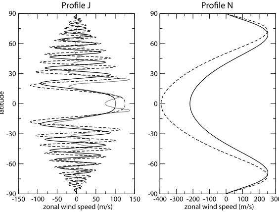
Figure 1: Zonal velocity measured at the surface in the planet’s mean rotat-ing frame for each of the four giants by trackrotat-ing cloud features in the outer weather layer. Profiles adapted from Porco et al. (2003), Sanchez-Lavega et al. (2000), Sromovsky et al. (2001) andSromovsky and Fry (2005).

et al., 2000). At higher latitudes, alternating prograde (eastward) and ret-rograde (westward) jets of smaller amplitude are observed extending all the way to the poles. These profiles are fairly symmetric with respect to the equator. On the ice giants (Uranus and Neptune) the picture is rather differ-ent. A very intense retrograde equatorial current is present with maximum velocity of 100 m/s on Uranus (Sromovsky and Fry,2005) and 400 m/s on Neptune (Sromovsky et al., 2001). At higher latitudes, a single prograde jet of large amplitude is present in each hemisphere. Several decades of ob-servations show that these zonal flows remain approximately steady (Porco et al.,2003).

The origin of these zonal flows and the associated question of the depth to which they extend into the planets’ interiors have been areas of ac-tive research in rotating fluid dynamics for several decades (e.g. Jones and Kuzanyan,2009, and references therein; see also the review byVasavada and

Showman, 2005). In particular, several models have been proposed to

near cloud level. These models are able to reproduce the high latitude struc-tures with alternating eastward and westward jets and a strong equatorial current (e.g. Williams, 1978; Cho and Polvani, 1996). These models tend to produce a retrograde equatorial jet (Yano et al.,2003), so they provide a plausible explanation for the retrograde equatorial flow of the ice giants but not for the prograde flow observed on gas giants. A parametrized forcing such as a strong equatorially-localized baroclinicity is required to force a shallow system to produce a prograde equatorial jet (Williams,2003). The second class of models is deep convection models which simulate most or all of the whole 104km-thick molecular hydrogen layer (Busse,1976;

Chris-tensen, 2001, 2002; Manneville and Olson, 1996). The presence of deep

convection is inferred from the observation that the atmospheres of the ma-jor planets emit more energy by long-wave radiation than they absorb from the Sun. Consequently their atmospheres must receive additional heat sup-plied by the interior of the planet. Recent numerical models using either a Boussinesq approximation (Heimpel et al.,2005) or an anelastic approx-imation (Jones and Kuzanyan,2009) and low Ekman numbers (i.e. strong rotational effect compared with viscous dissipation) display alternating zonal jets at high latitudes. A strong eastward equatorial jet is a robust feature of these models where the Coriolis force dominates buoyancy, in good agree-ment with the gas giant observations. Interestingly, deep convection models suggest that the zonal velocity generated by non-linear interactions of con-vective motions (i.e. the motions directly forced by buoyancy) is roughly geostrophic, that is, invariant along the direction of the rotation axis. This feature is also present in strongly compressible models provided that the Ekman number is small enough, despite the increase of density with depth yielding ageostrophic convective motions (Jones and Kuzanyan,2009;Kaspi et al.,2009). When the convection is more vigorous such that the buoyancy force overcomes the Coriolis force, 3D turbulence homogenizes angular mo-mentum; a retrograde jet forms in the equatorial region and a single strong prograde jet forms in the polar region, in good agreement with the ice giant observations (Aurnou et al.,2007).

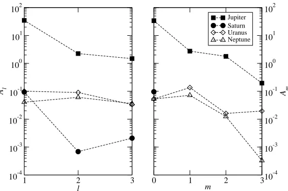
Another feature of the giant planets is their strong magnetic fields (fig-ure2). The observed magnetic fields for gas and ice giants differ drastically (see for instance the recent review byRussell and Dougherty,2010). Jupiter and Saturn have a main axial dipole component (corresponding to l = 1, m= 0 in figure 2), a feature shared with the Earth for instance (Yu et al.,

2010; Burton et al., 2009). Neptune and Uranus, on the other hand, have

0 1 2 3

m

10-4 10-3 10-2 10-1 100 101 102

Am

1 2 3

l

10-4 10-3 10-2 10-1 100 101 102

Al

Jupiter Saturn Uranus Neptune

Figure 2: Spectra of the magnetic field squared amplitude at the planetary radius for degrees l and order m up to 3 obtained from inversion models of the magnetic measurements. The squared amplitude for a given degree l is Al=Plm=0(l+ 1)

(gm_l )2+ (hm_l )2

using a Schmidt normalisation for the spherical harmonics. The squared amplitude for a given mode m is Am=Plmaxl=m(l+ 1)

(g_lm)2+ (hm_l )2

. gm_l and hm_l are the Gauss coefficients in gauss. After Yu et al. (2010) (Model Galileo 15), Burton et al. (2009) (Cassini measurements), Connerney et al. (1991) (model O8) and Herbert

Herbert, 2009). The magnetic field is generated in the deep, electrically conducting regions of the planets’ interiors: a metallic hydrogen layer for Jupiter and Saturn (Nellis et al.,1999;Guillot,2005, and references therein) and an electrolyte layer composed of water, methane and ammonia ( Hub-bard et al., 1991; Nellis et al., 1997) or superionic water (Redmer et al.,

2011) for Uranus and Neptune.

Numerical models of convective dynamos in rapidly rotating spherical shells typically produce axial dipolar dominated magnetic fields for moder-ate Rayleigh numbers and modermoder-ate Ekman numbers (e.g.Olson et al.,1999;

Aubert and Wicht,2004;Christensen and Wicht,2007). To explain the un-usual large scale non-dipolar magnetic fields of Uranus and Neptune, models using peculiar parameter regimes or different convective region geometries have been proposed. The latter models show that a numerical dynamo op-erating in a thin shell surrounding a stably-stratified fluid interior produces magnetic field morphologies similar to those of Uranus and Neptune ( Hub-bard et al.,1995;Holme and Bloxham, 1996; Stanley and Bloxham, 2006).

G´omez-P´erez and Heimpel (2007) obtain weakly dipolar and strongly tilted dynamo magnetic fields when high magnetic diffusivities are used (or equiv-alently small electrical conductivity). Their results show that these peculiar fields are stable in the presence of strong zonal circulation and when the flow has a dominant effect over the magnetic fields. This feature is also empha-sized byAubert and Wicht(2004) who find stable equatorial dipole solutions with a weak magnetic field strength and low Elsasser number (measure of the relative importance of the Lorentz and Coriolis forces) for moderately low Ekman numbers. They argue that the magnetic field geometry of the equa-torial dipole solution is incompatible with the columnar convective motions and thus this morphology is stable only when Lorentz forces are weak.

Although scaling laws derived from numerical simulations of dynamos driven by basal heating convection predict dipolar magnetic field in plan-etary parameter regimes (Olson and Christensen, 2006), recent numerical simulations using more realistic parameter values (lower Ekman numbers) have not produced large scale magnetic fields so far, and require larger mag-netic Reynolds numbers (measure of magmag-netic induction versus magmag-netic diffusion) (Kageyama et al., 2008). Moreover, convection in the interior of Jupiter is often thought to be driven by secular cooling (Stevenson, 2003). Numerical dynamos driven by secular cooling typically produce weak dipole or multipolar magnetic field for larger forcing (Kutzner and Christensen,

re-mains open.

The dichotomies observed in the magnetic fields and in the zonal wind profiles of the giant planets are rather striking. Up to now no study has tried to relate them directly, probably because the former is a feature of the deep interior whereas the latter is a characteristic of the surface. However, if some mechanism is able to transport angular momentum from the surface down to the deep, fully conducting region then the zonal motions may influence the generation of the magnetic field. In the non-magnetic deep convection models (Heimpel et al., 2005; Jones and Kuzanyan, 2009), zonal motions extend geostrophically throughout the electrically insulating molecular hy-drogen layer down to the bottom of the model. On the other hand, due to the possible rapid increase of electrical conductivity with depth in the outer region, Liu et al. (2008) argued that the ohmic dissipation produced by geostrophic zonal motions shearing dipolar magnetic field lines would ex-ceed the luminosity measured at the surface of Jupiter if the vertical extent of this geostrophic zonal motions exceeds 4% of the planet radius. However, the argument ofLiu et al. (2008) is purely kinematic, that is the action of the magnetic forces on the flow and the feedback on the magnetic field are ignored. In a self-consistent magnetohydrodynamic model, the zonal flow would adjust toward a non-geostrophic state due to the action of magnetic forces if the electrical conductivity of the fluid is significant (Glatzmaier

(2008), see also the non-linear numerical simulations of convectively-driven dynamos ofAubert(2005)). In this case, angular momentum may be trans-ported along the magnetic field lines leading to a dynamical state close to the Ferraro state. This state minimizes the ohmic dissipation produced by the shearing of the poloidal magnetic field by the zonal flow as the poloidal magnetic field lines are aligned with angular velocity contours. Both scenar-ios, either geostrophic zonal balance or Ferraro state, imply the existence of multiple zonal jets of significant amplitude at the top of the fully conducting region beneath. The plausibility of each scenario depends on the radial pro-file of electrical conductivity, which is currently not well constrained within the giant planets (Nellis et al., 1999).

in-stabilities. These instabilities are able to generate large scale magnetic fields, and so they are an interesting source of dynamo action under planetary in-terior conditions. In order to test the plausibility of a dynamo driven by this source in isolation, we use an incompressible 3D numerical dynamo model with a zonal velocity profile imposed at the top of a spherical shell contain-ing a conductcontain-ing fluid. We use a dynamical approach, that is non-linear interactions between the flow and the magnetic field are taken into account; therefore the fluid flow is free to adopt a three-dimensional structure as long as it satisfies the imposed viscous boundary conditions.

The dynamics of the deep conducting region is usually assumed to be slower than the dynamics of the outer molecular hydrogen region due to magnetic braking, even if uncertainties remain in the electrical conductivity. The model presented in this paper assumes an idealized one-way coupling between the outer and deep regions. A more realistic model would need to account for the back reaction of the deep layer onto the outer layer; a study of the consistent dynamical interaction of the two layers is beyond the scope of this paper. For studies of more realistic coupling, see promising recent numerical models of self-consistent convectively-driven dynamos in spheri-cal shells including radially variable electrispheri-cal conductivity ofHeimpel and G´omez P´erez (2011) and Stanley and Glatzmaier (2010). In these models, slow convective motions in the interior dynamo region coexist with strong zonal flow near the outer surface. Differential rotation in the interior is only partially inhibited by the strong magnetic field.

In order to assess the role of the zonal wind profile on the topology of the sustained magnetic field, we use both Jupiter-like and Neptune-like zonal wind profiles. In the giant planets, as in rocky planets, it is usually assumed that the dynamo mechanism is driven by convective motions. The giant planets display a strong surface heat flux (with the exception of Uranus) meaning that heat transfer is efficient in the interior of the planet and thus mostly due to convection (Guillot and Gautier,2007, and references therein). Here we want to assess the efficiency of zonal velocity forcing alone, so we do not model convective motions.

The first goal of this work is to quantify what amplitude of the zonal wind insidethe conducting layer is needed to trigger the dynamo instability, so we do not model the exact or realistic coupling between the molecular hydrogen upper layer and the deep, electrically conducting region. Our second goal is to test to what extent the pattern of the zonal flow imposed at the top of the conducting layer influences the topology of the self-sustained magnetic field.

Then we present numerical results from simulations in the non-magnetic case (section 3) followed by results from dynamo simulations (section 4). The application of our results to planetary conditions is discussed in section 5.

2

Model

We model the deep conducting layer of the giant planets as a thick spher-ical shell. At the top of the conducting layer we impose an axisymmetric azimuthal velocity to represent the zonal flow generated in the overlying en-velope. The shell rotates around thez-axis at the imposed rotation rate Ω. The aspect ratio isγ =ri/rowhereriis the inner sphere radius,

correspond-ing to a rocky core, and ro the outer sphere radius, corresponding to the

top of the fully conducting region. The fluid is assumed incompressible with constant densityρ and constant temperature, that is, no convective motions are computed. The assumption of incompressibility is made for simplicity, although the pressure scale height at the depths of the conducting layer is roughly 8000km (Guillot et al.,2004), that is, about 1/5 of the thickness of the layer. The effects of compressibility may well play a role in the dynamics of the conducting regions (see for instanceEvonuk and Glatzmaier, 2004).

if the magnetic forces upset the zonal geostrophic balance. Depending on the magnitude and radial profile of the electrical conductivity, the amplitude of the zonal motions might be reduced, and the zonal flow contours would tend to align with the magnetic field lines, although we do not expect the characteristics of the zonal jets (narrow or wide, relative amplitude of the peaks) to be altered very much.

We use two different synthetic azimuthal velocity profiles for the bound-ary forcing imposed at the top: a multiple jet profile for the gas giants with a profile based on Jupiter’s surface zonal winds (hereafter profile J) and a 3-band profile based on Neptune’s surface zonal winds (profile N).

For Jupiter, we use the profile given in Wicht et al. (2002)

U=U(s)eφ=U0

s r0cos(n0π)

cos

n0π

s−r0

rs−r0

eφ, (1)

wheres=rsinθ,rsis the surface radius of the planet andU0=U(r0, θ=π/2).

n0 controls the numbers of jets. The profile at the radius rs best matches

the observed profile at the surface forn0 = 4 (figure3). The profileU(ro, θ)

is used to drive the flow at the top of our simulated metallic hydrogen layer (figure3). The ratio γs =rs/ro determines the U profile at ro. We choose

γs=rs/ro = 1/0.8 = 1.25 following Guillot et al.(1994).

For the Neptune-like profile, we use the zonal velocity profile measured at the surface of Neptune, approximated by a polynomial of order 10 in latitude. We project this surface velocity profile geostrophically down toro

usingγs= 1/0.85 = 1.18 (Hubbard et al.,1991) (figure3).

The existence of a rocky core at the centre of the giant planets is un-certain and depends on the poorly constrained composition of the planet. Estimates for the core mass are 0₋14m⊕ for Jupiter (total mass 318m⊕), 6−17m⊕for Saturn (total mass 95m⊕) and 0−4m⊕for Uranus and Neptune (total mass 15m⊕ and 17m⊕ respectively) where m⊕ denotes the mass of the Earth (Guillot,2005). If present, the rocky cores are therefore believed to be small. Following the interior model of Jupiter proposed by Guillot et al.(1994) we use an aspect ratio ri/ro = 0.2 for all the simulations

per-formed. The inner core is assumed to be electrically conducting, with the same conductivity as the fluid in the conducting layer. We did not carry out simulations with an insulating core as the effect of the conductivity of the inner core on the dynamo mechanism is believed to be small (Wicht,2002). The velocity boundary condition is no-slip at the inner boundary.

The velocity u is scaled by U0, the absolute value of the azimuthal

Figure 3: Zonal velocity profile imposed at the surface of model J (left) and model N (right) (solid lines). Both profiles are obtained by assuming that the zonal velocities are geostrophic for rs > r > ro and using the profile

represented by a dashed line at the surface of the planet (r = rs): model

J, profile (1) with n0 = 4, γs = rs/ro = 1.25 and U0 = 100; model N:

polynomial fit of order 10 in latitude of the zonal wind profile measured at the surface of Neptune (figure1) with γs = 1/0.85 = 1.18. For comparison

whereρ is the fluid density andµ0 is the vacuum magnetic permeability.

We numerically solve the momentum equation for an incompressible fluid,

Re∂u

∂t +Re(u·∇)u+ 2

Eez×u=−∇p+∇ 2

u+ 1

E (∇×B)×B, (2)

the continuity equation,

∇_{·u= 0, (3)}

and the magnetic induction equation,

∂B

∂t =∇×(u×B) + 1 ReP m∇

2

B, (4)

∇_{·B= 0, (5)}

wherepis the dimensionless pressure, which includes the centrifugal poten-tial.

The Reynolds numberRe=roU0/ν parametrizes the mechanical forcing

exerted on the system by controlling the amplitude of the zonal velocity. The magnetic Prandtl number P m = ν/η measures the ratio of viscous to magnetic diffusivities. The magnetic Reynolds number Rm is defined as Rm = ReP m. The Ekman number E = ν/(Ωr2_o) measures the im-portance of the viscous term over the Coriolis force. The Rossby number Ro=ReE =U0/(Ωro) is the ratio of inertial force to Coriolis force. Note

that in our definition the Rossby number refers to the amplitude of the pre-scribed zonal jets at the surface, and not to the local flow velocity.

The results presented in this paper were obtained with the PARODY code, a fully three-dimensional and non-linear code. The code was derived from

Dormy(1997) by J. Aubert, P. Cardin, E. Dormy in the dynamo benchmark

3

Dynamics without the magnetic field

For a rapidly rotating system in which the Coriolis force exactly balances the pressure force, the Proudman-Taylor constraint states that the flow is z-invariant and follows geostrophic contours. For an incompressible fluid in a bounded container, these geostrophic contours correspond to surfaces of equal height. In a sphere the only geostrophic motions are azimuthal and axisymmetric. In the giant planets’ conducting envelopes, the Ekman number is about 10−₁₆

and the Rossby number is much smaller than 1 (Guillot et al., 2004). In the absence of a magnetic field, we expect the Proudman-Taylor constraint to hold for large scale motions. As we want to reach the dynamical regime in which the flow is strongly geostrophic, the use of small Ekman and Rossby numbers is required. We carried out simulations for 10−5 _{> E >10}−6 _{for model J and 10}−5 _{> E >5}

×10−6 _for

model N. The Rossby numbers are always smaller than 0.1. For the profile J, in cases of low Ekman numbers (E ≤2×10−6_{), we imposed longitudinal}

symmetry by calculating only the harmonics of a chosen order ms. The

required resolution forE= 10−₆

is 500 points on the radial grid andl= 580 spherical harmonics degrees.

3.1 Axisymmetric flow

When the imposed boundary forcing is small enough,i.e.when the Rossby number Ro is less than a critical value Roc, the flow is axisymmetric and

−0.5 0 0.5

(a) Model J

0 1 2 3 4

(b) Model N

Figure 4: Angular velocity uφ/(rsinθ) (left) and streamlines of the

merid-ional circulation (isocontours ofψ=rsinθ∂up_∂θ withup the velocity poloidal

scalar) (right) of the axisymmetric flow in the northern meridional plane. For the meridional circulation, anti-clockwise (clockwise) flows are shown in solid (dotted) lines. The parameter for the simulations are E = 5_×10−₆ and Ro= 0.015 for model J (a) and E = 10−5 _{and Ro= 0.02 for model N}

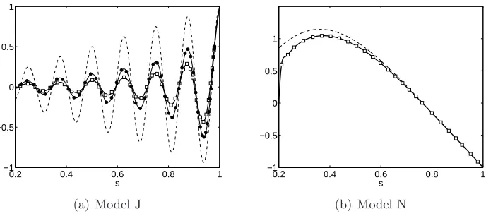
0.2 0.4 0.6 0.8 1 −1

−0.5 0 0.5 1

s

(a) Model J

0.2 0.4 0.6 0.8 1

−1 −0.5 0 0.5 1

s

(b) Model N

Figure 5: Zonal velocity in the equatorial plane for subcritical numerical simulations (solid lines) compared to the zonal velocity at radiusr= 0.98ro

(symbols) and imposed velocity at the top (dashed line) both projected in the equatorial plane for (a) model J (E= 5×10−6 _{(bold solid line and open}

squares) andE = 10−6 _{(thin solid line and black circles)) and (b) model N}

(E = 10−₅

(bold solid line and open squares)).

in the whole volume. The comparison between the zonal velocity just below the Ekman layer and in the equatorial plane (figure5) shows that the zonal velocity is geostrophic in the bulk of the fluid (outside of the boundary lay-ers). For model N (figure5(b)), the zonal jets are wider, so the zonal flow already displays a strong geostrophic structure atE= 10−5_{. Note that the}

azimuthal velocity has to match the no-slip boundary condition at the inner core, and so an internal Stewartson layer forms on the axial cylinder tangent to the inner core (Stewartson,1966).

3.2 Non-axisymmetric motions

3.2.1 Model J

Rossby wave at the onset When the boundary forcing (measured by Ro) becomes greater than a critical value Roc, the axisymmetric basic flow

Figure 6: Non-zonal axial vorticity in the equatorial plane (right) and in a meridional slice (left) for model J atE = 4×10−6 _{and Ro= 1.01Ro}

c (blue:

negative and red: positive). The black curve represents the zonal velocity in the equatorial plane.

by the zonal flow velocity varies withs, implying that it is a single wave.

Wicht et al. (2002) studied the linear stability of the imposed zonal flow (1) in a spherical shell modeling the insulating molecular hydrogen layer of Jupiter (aspect ratio 0.8). ForE = 10−4 _{they found nearly bidimensional}

instabilities that they described as drifting columns aligned with the rotation axis and similar to convective solutions. Although they do not identify these instabilities as waves, their characteristics are very similar to the ones obtained with our non-linear model.

The nearlyz-invariant structure and the prograde drift are two character-istics of Rossby waves propagating in a spherical container. The dispersion relation for the Rossby wave given by a local linear analysis is (e.g. Finlay,

2008)

ωrw(s) =−2Ωβ m/s

k2

s+ (m/s)2

, (6)

where β = h−1_{(dh/ds) = −s/(r}2

o −s2) is related to the slope of the upper

boundary of the spherical container of height h. ks and m/s are the

ra-dial and azimuthal wavenumbers respectively. The theoretical Rossby wave frequencyωrw can be calculated at a given radius assuming ks ≈m/s and

(s2 = 0.87) is the smallest (resp. largest) radius where a significant

vortic-ity associated with the presence of the wave can be seen in the numerical calculations. This strongly indicates that the shear instability occurs as a Rossby wave.

The velocity of the zonal flow U enters the dispersion relation of the Rossby wave through a Doppler shift

ω(s) =ωrw(s) +U(s)

m

s. (7)

As reported earlier,ω(s) is constant in our numerical calculations soωrw(s)

must adapt in the s-direction for the wave to be coherent. In a prograde jet U > 0, ωrw must decrease, which requires a local increase in ks in

equation (6) and so a local decrease in the radial lengthscale, which can be observed in figure 6. For small enough Ekman number (in practice E < 5_×10−6_{), the critical wavenumber m}

c of the Rossby mode is

inde-pendent of E. The radial lengthscale is determined by the width of the jet and the vortices are roughly circular in the equatorial plane (figure 6) suggesting thatmc is controlled by the width of the jets.

In a local approximation that neglects the curvature terms, a criterion of instability of barotropic shear flows has been derived byIngersoll and Pollard

(1982) for an anelastic model in a full rotating sphere and byKuo(1949) for thin stably stratified “weather” layers. Using an inviscid Boussinesq model and for barotropic instability of a zonal flow U in a sphere, this necessary condition implies a change of sign of a quantity ∆ at some radius:

∆ = 2β₋Rodζ

ds, (8)

whereζ is the vorticity of the zonal flow,

ζ = dU ds +

U

s. (9)

that the local criterion does not predict the location of global saturated modes.

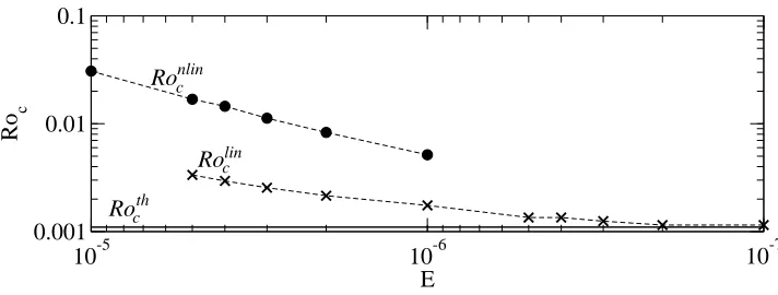
The theoretical critical Rossby number obtained from applying the crite-rion (8) to the profile (1) imposed at the top of model isRoth_c = 0.0011. The threshold of the first instability of the axisymmetric flow, denoted Ronlin

c ,

obtained with the numerical simulations are shown in figure7. Despite the decrease ofRonlin_c with the Ekman number,Ronlin_c is still about four times larger thanRoth_c forE= 10−6 _{because the amplitude of the zonal flow within}

the bulk is reduced by viscous boundary layers in the numerical simulations. Due to computational limitations, it is not possible for us to carry out simu-lations at smallerEwith a fully non-linear code and prove the existence of an asymptotic regime for the inviscid instability threshold. For this purpose we used a dedicated linear code described inA. The linear code calculates lin-ear perturbation solutions to the momentum equation using the geostrophic profileU as the basic flow in the bulk of the fluid. The computational time is greatly reduced by the linear approach but is restricted to an analysis of the instability threshold. The growing solutions obtained with the linear code exhibit very similar features to the Rossby waves in the non-linear sim-ulations (frequency, bidimensional structure, radial extent, location of the maximum amplitude in a retrograde jet). In figure 7 the threshold Rolin_c obtained with the linear code approaches asymptotically the value given by the local theory. For the same Ekman number,Rolin_c is smaller than Ronlin_c since the geostrophic zonal flowU is used in the linear code, that is the jets in the bulk have greater amplitude than in the non-linear code. From our linear computations we conclude that the theoretical criterion (8) is relevant to explain the onset of instability obtained numerically. More details about the onset of the hydrodynamic instability can be found inGuervilly (2010). The characteristic time of the Rossby wave isτrw = 1/ω. At the

instabil-ity threshold, the numerical simulations giveτrw ≈18Ω−1 forE <5×10−6.

The timescale of the zonal jets isτzj =ro/U0 = Ω−1/Ro. ForRo= 0.01, we

have τzj > τrw: the Rossby wave propagation is faster than the advection

of the fluid by the zonal flow. The turnover time of a fluid particle trapped in a Rossby wave is τto = l/Vs where l is the typical radial displacement

of the particle andVs the typical cylindrical radial velocity of the particle.

AtRo= 1.01Roc,Vs is typically 10−2U0. In a rough approximation we use

l=δ, where δ is the width of the jets, δ _≈0.1ro for the profile J. Then we

obtain τto ≈0.1ro/(10−2U0) ≈10Ro−1Ω−1 ≈103Ω−1: the turnover time of

10-7 10-6

10-5

E 0.001

0.01 0.1

Ro

c

Ro

Ro

Ro

nlin c

lin c

c th

Figure 7: Critical Rossby number obtained from fully non-linear numerical simulations for model J (Ronlin_c , circles) compared to the theoretical Rossby number obtained with the local instability criterion (8) using the geostrophic profile (1) U(s, θ = π/2) (Roth

c , black line). The critical Rossby number

obtained from the linear numerical calculation is also shown (Rolin_c , crosses).

thanδ and so the turnover time is slightly overestimated here.

Supercritical regime When the Rossby number is increased in the su-percritical regime, other prograde jets will eventually become unstable. A second Rossby wave appears in the weakly supercritical regime, at Ro = 1.06Roc for E = 5×10−6, with a maximum velocity located in the

retro-grade zonal jet at larger radius than the first wave maxima (i.e. the wave appearing for Ro = Roc) (figure 8(a)). To fill the larger circumference at

larger radius the instability has a slightly larger wave number, m = 22 in-stead of 21, while the radial width of the jet is comparable. The second wave propagates faster, in agreement with the Rossby wave dispersion re-lation (6). Barotropic instabilities tend to broaden and weaken narrow jets by redistributing potential vorticity (see for instance Pedlosky,1979). The smoothing of the jets saturates the amplitude of the Rossby waves. For this slightly supercritical regime the zonal flow profile is only weakly modified. Upon further increasing the forcing (Ro= 2.94Roc), several Rossby waves of

different wavenumbers superpose and interact (figure 8(b)). The structure of the waves and the jets is still mainly bidimensional except in the viscous boundary layers. The typical cylindrical radial velocity is Vs ≈ 0.1U0 and

the Rossby number is 0.05 so the turnover time is about 20Ω−1 _assuming

that the radial displacement l = δ, about the same order of magnitude as the timescale of the zonal jets.

(a) Ro_{= 1}.₀₆Ro_c

u r

−0.1 −0.05 0 0.05 0.1

u_φ

−0.2 −0.1 0 0.1 0.2

(b)Ro= 2.94Ro_c

Figure 8: Snapshots of the radial (left) and azimuthal (right) velocity com-ponents in the equatorial plane for E = 5_×10−6 _{and Ro > Ro}

c for model

J. The velocities are scaled byU0. Foruφthe colorscale has been truncated

(uφ(ro, θ = π/2, φ) = 1). The black curve represents the zonal velocity in

(a)

1 2 3 4 5 6

Ro/Ro_c

0 0.1 0.2 0.3 0.4

(V_s2+V_φ2)1/2

V_φ

V_s

V_φm=0

(b)

Figure 9: (a) Time-averaged zonal velocity in the equatorial plane for E= 5_×10−₆

and different forcings. (b) Amplitude of the non-axisymmetric radial velocity Vs (squares), non-axisymmetric azimuthal velocity Vφ

(cir-cles), non-axisymmetric velocity (V_s2+V_φ2)1/2 (diamonds) and zonal veloc-ity at the radius s = 0.75 (triangles). All velocities were measured in the equatorial plane in the units ofU0. The amplitude of the non-axisymmetric

velocity corresponds to the maximum in a snapshot, whereas the zonal ve-locity amplitude has been averaged in time.

plotted for different Ro up to Ro = 5.88Roc. As the forcing is increased,

the Rossby waves gradually reduce the jet strength and broaden the jet width. For Ro = 2.94Roc, the retrograde jet at s = 0.81 has been mostly

destroyed leading to the widening of the zonal jet width. We note that the zonal flow becomes mostly westward for the strongest forcings. The amplitude of the zonal flow located at s > 0.9 is hardly affected because the threshold to destabilise the outermost jets is high due to the large slope (related toβ in equation (8)). For Ro <2.35Roc, the amplitude of the

non-axisymmetric velocity, relative toU0, increases with the forcing (figure9(b)).

After reaching a maximum, at Ro = 2.35Roc, the amplitude of the

non-axisymmetric flow decreases relative toU0. The “efficiency” of the forcing

to drive the non-zonal velocity is reduced as the Rossby waves smooth the gradient of vorticity and so affect their excitation mechanism.

Figure 10: Non-zonal axial vorticity in the equatorial plane (right) and in a meridional slice (left) for model N atE = 5_×10−6 _{andRo= 1.01Ro}

c (blue:

negative and red: positive). The black curve represents the zonal velocity in the equatorial plane.

3.2.2 Model N

The shear instability takes the form of anm= 2 oscillation in the azimuthal direction (figure 10). It is a single wave propagating eastward with the same frequency over the shell, and is nearly z-invariant. The maxima of the non-zonal vorticity are located on each side of the prograde jet. The characteristics of this wave are similar to the Rossby wave obtained with model J. The frequency of this wave is in agreement with the frequency of a theoretical Rossby wave of wavenumber m = 2 propagating at a radius s = 0.53 (assuming that ks ≈ m/s in the dispersion relation (6)). For

E = 10−₅

and E = 5_×10−₆

, the critical Rossby numbers obtained with the non-linear numerical simulations are respectively Ronlin_c = 0.0335 and Ronlin_c = 0.0325. Using the instability criterion (8) with the profile imposed at the surface we obtain a critical Rossby number of 0.026 in good agreement with the non-linear numerical results when the Ekman number decreases.

4

Magnetic field generation

The non-axisymmetric motions are of prime importance for the dynamo mechanism because a purely toroidal flow cannot generate a self-sustained magnetic field. We note that some axisymmetric poloidal flow is present when Ro < Roc as a weak meridional circulation is created by the Ekman

numbers so we do not expect to find dynamos when the zonal flow is stable, that is when Ro < Roc, in the asymptotic inviscid regime. Indeed we did

not find dynamos whenRo < Roc (up toP m= 10). The non-axisymmetry

associated with the hydrodynamic shear instability is a crucial element for the dynamo process: the stable zonal flow cannot sustain a magnetic field by itself. This is in agreement with the results obtained byGuervilly and Cardin(2010) with dynamos generated by spherical Couette flows (differen-tial rotation between two concentric spheres).

4.1 Characteristics of the magnetic field for model J

We have performed dynamo simulations for Ro= 1.17₋1.76Roc and E =

5×10−6_{. We find that the dynamo threshold occurs at a rather high value}

of the magnetic Prandtl number,P mc ≈5. The critical magnetic Reynolds

number (defined via the maximum forcing velocity) required for dynamo action isRmc ≈20,000 (see section5for an estimate of the critical magnetic

Reynolds number defined via the local velocity). For a given forcing, we have performed calculations just above the critical magnetic Prandtl number, P mc, and up to 2P mc.

The main features of the self-sustained magnetic field can be observed in figures 11 and 12. The magnetic field displays a dipolar symmetry, i.e. antisymmetry with respect to the equatorial plane,

(Br, Bθ, Bφ)(r, π−θ, φ) = (−Br, Bθ,−Bφ)(r, θ, φ). (10)

(a) Axisymmetric magnetic field

Br

-2.568 -1.8₃₄-1.101

-0.367

0.367 1.101

1.834 2.568

(b) Radial magnetic field atr_s

Figure 11: Magnetic field for model J. (a) Snapshot of the axisymmetric magnetic field in a meridional plane: magnetic poloidal field lines (left) and azimuthal magnetic field (right) (blue: negative and red: positive). (b) Map of the radial magnetic field at the surface of the planetrs= 1.25ro in

unit of 10−₃√

ρµ0U0 (solid line: positive and dotted line: negative). The

poloidal magnetic field atr=rs is calculated assuming the region between

ro and rs is electrically insulating. The parameters of this simulation are

E= 5_×10−6_{,Ro= 1.17Ro}

1 20 40 60

l

10-8 10-7 10-6 10-5 10-4 10-3 10-2 10-1

KE toroidal KE poloidal ME toroidal ME poloidal

0 10 20 30

m

10-8 10-7 10-6 10-5 10-4 10-3 10-2 10-1

(a) Kinetic and magnetic energies in the fluid

1 20 40 60

l

10-20 10-18 10-16 10-14 10-12 10-10 10-8 10-6

0 10 20 30 40

m

10-20 10-18 10-16 10-14 10-12 10-10 10-8 10-6

(b)A_landA_matr_s

Figure 12: Magnetic energy spectra for model J. (a): Kinetic (KE) and magnetic (ME) energy per unit volume for each spherical harmonics degree l (left) and mode m (right) in the fluid conducting region given in unit of ρU2

0. (b): Squared amplitudes of the magnetic field, Al (left) and Am

(right) as defined in figure 2, at rs = 1.25ro given in unit of ρµ0U02. Only

generates a magnetic field of small latitudinal scale that decreases rapidly with radius.

The spectrum and map of the radial magnetic field at the surface of our modeled planet (at radius rs = 1.25ro) (Figs. 11(b) and 12(b)) show that

the magnetic field is strongly dominated by the axial dipole. The magnetic field generated at the scale of the Rossby wave (m = 22) is still visible in the spectrum of the magnetic field but its amplitude is weak at this radius: about four orders of magnitude smaller than the amplitude of the axisymmetric mode (note that the spectrum in figure 12(b) represents the squared amplitude of the field).

In all the simulations performed, no inversion of polarity of the axial dipole has been observed. The tilt of the dipole is rather weak, at most 2◦ from the rotation axis. We found a secular variation of the dipole axis of about 1◦

every 1000 rotation periods or alternatively 0.001 global magnetic diffusion time.

Just above the dynamo threshold (P mc < P m 62P mc), the magnetic

field is weak: the magnetic energy contained within the fluid conducting region is only about 5% of the kinetic energy. The magnetic field does not strongly act back on the flow, except to produce its own saturation. A comparison between the zonal flow in the non-magnetic case and in the presence of the dynamo magnetic field does not reveal significant differences. The magnetic field lines of the poloidal field are almost aligned with the rotation axis and the flow structure (see figure11(a)) so the flow disruption due to Lorentz forces is weak.

4.2 Characteristics of the magnetic field for model N

We performed simulations at Ro = 1.05₋1.5Roc and E = 10−5. We find

the dynamo threshold atP mc ≈1, that is, the critical magnetic Reynolds

number isRmc≈4000.

The main features of the self-sustained magnetic field can be observed in figures13 and 14. The self-sustained magnetic field displays an equatorial symmetry,i.e.

(Br, Bθ, Bφ)(r, π−θ, φ) = (Br,−Bθ, Bφ)(r, θ, φ). (11)

(a) Axisymmetric magnetic field

Br

-1.350 -1.350

-1.350 -1.350 -0.450

-0.450

-0.450

-0.450

0.450

0.450

0.450

0.450 1.350

1.350

(b) Radial magnetic field atr_s

Figure 13: Magnetic field for model N (same as figure 11). For the ax-isymmetric azimuthal field, blue corresponds to negative values and red to zero values. The radial magnetic field is plotted at the surface of the planet rs = 1.18ro in unit of 10−5√ρµ0U0. The parameters of this simulation are

E= 10−5_{,Ro= 1.20Ro}

1 20 40 60

l

10-12 10-10 10-8 10-6 10-4 10-2 100

KE toroidal KE poloidal ME toroidal ME poloidal

0 2 4 6 8 10

m

10-12 10-10 10-8 10-6 10-4 10-2 100

(a) Kinetic and magnetic energies in the fluid

1 10 20 30 40 50 60

l

10-22 10-20 10-18 10-16 10-14 10-12 10-10 10-8

0 2 4 6 8 10

m

10-22 10-20 10-18 10-16 10-14 10-12 10-10 10-8

(b)A_landA_matr_s

(l, m) = (2,0) (axial quadrupole) and (l, m) = (4,0) modes. At the sur-face of the planet (figure 14(b)), the magnetic field appears to be mainly axisymmetric (with thel= 2 andl= 4 harmonics degrees dominant). The amplitude of the m = 2 structure is weak, about two orders of magnitude smaller than them= 0 mode but still visible at high latitudes on the map of the radial field at the surface (figure13(b)).

Due to the equatorial symmetry of the field, the magnetic field lines in the equatorial plane are roughly perpendicular to the cylindrical structure of the flow whereas they are nearly aligned at higher latitudes (figure13(a)). As a result magnetic braking acting on the flow is stronger in the equato-rial region than at high latitude regions. In the simulation performed here (P mc < P m 6 2P mc), the magnetic energy is weak compared to the

ki-netic energy (about 5%) so the feedback of the magki-netic field on the flow remains weak. For a stronger magnetic field (at larger magnetic Reynolds numbers), we expect that the flow disruption would become important. As a result the equatorially symmetric solution may become unstable and the magnetic field may switch to an axial dipolar symmetry. This is the result obtained byAubert and Wicht(2004) in convectively-driven dynamos: they found equatorial dipolar magnetic fields for Rayleigh numbers close to the convection onset; these solutions become unstable as the convective forcing is increased and an axial dipolar configuration is preferred.

In summary, the flows driven by the profiles J and N produce very dif-ferent poloidal magnetic fields: mainly a strongly axisymmetric dipole for the profile J and a weak multipolar axisymmetric field dominated by the magnetic field induced at the scale of the Rossby waves for the profile N. In both cases the magnetic field within the conducting region is mainly an axisymmetric toroidal field. The different magnetic field morphology is quite surprising given that the flows are quite similar: strong zonal flows and propagating Rossby waves. In the next section we review the dynamo mechanism that has been proposed to operate for similar flows and suggest the key difference between profiles J and N that determines the topology of their self-sustained magnetic fields.

4.3 Dynamo mechanism

Rossby waves (of wavenumber about 10 for the Ekman numbers and Rossby numbers they investigated). The self-sustained magnetic field has a strong axisymmetric toroidal component and a mostly axisymmetric poloidal com-ponent. SC06 show that the time dependence of the flow is a key ingredient for the dynamo effect: time-stepping the magnetic induction equation using a steady flow taken either from a snapshot or a time-average leads to the decay of the magnetic field. They characterize the dynamo process as an αω mechanism. In mean field theory, the α effect parameterizes the gen-eration of an axisymmetric poloidal magnetic field from the correlation of small scale magnetic field and velocity. The α effect usually requires that the flow possess some helicity, the correlation between fluid velocity and vorticity,H=u_·ω (e.g.Moffatt,1978). Flows displaying a columnar struc-ture aligned with the axis of rotation, such as Rossby waves or convection columns (Olson et al., 1999), typically possess strong mean helicity. As these columns are essentially bidimensional vortical structures, the helicity is mainly produced by the term uzωz. In nearly z-invariant flow, the axial

(z) velocity is mostly due to two terms: the slope effect and the Ekman pumping. The slope effect comes from the combination of mass conserva-tion and impenetrable boundaries: a (cylindrical) radial velocity us creates

an axial velocity uz ∼ zβus with β = h−1(dh/ds). In the limit of rapid

rotation in a spherical container, this contribution is much larger (of order 1) than the Ekman pumping (uz ∼E1/2ωz). However, the axial velocity

produced by the slope effect is phase shifted by π/2 with ωz, and so does

not allow the production of mean helicity. On the contrary, axial velocity produced by Ekman pumping is in phase with the axial vorticity and a dy-namo mechanism based on the Ekman pumping associated to an azimuthal necklace of axial vortices is plausible (Busse, 1975). In a numerical experi-ment at small Ekman numbers (E=O(10−8_{)), SC06 artificially remove the}

Ekman pumping and observe dynamo action with nearly the same threshold showing that the Ekman pumping is unimportant in their dynamo mecha-nism. The crucial importance of the time dependence of the flow and the negligible contribution of the Ekman pumping lead SC06 to consider the in-volvement of the Rossby waves in the dynamo process. They conjecture that the propagation of the Rossby waves yields a proper phase shift between the non-axisymmetric magnetic field and velocity field in order to produce the axisymmetric poloidal magnetic field.

theαtensor, which are the relevant coefficients for theαeffect, are non-zero if and only if the flow pattern is drifting relative to the mean flow.

Tilgner(2008) explains that the time dependence of a velocity field can lead to dynamo action even when any particular snapshot of the velocity field cannot because the linear operator associated with the induction equation is non-normal. In particular, he shows that the simple time dependence of a propagating wave is enough for dynamo action. Several numerical studies report the importance of the time dependence of the velocity field, mainly of oscillating nature (Reuter et al.,2009;Gubbins,2008).

The idea that the propagation of Rossby waves may maintain a dynamo action is very appealing as their presence is ubiquitous in rotating fluid dy-namics. A system in which no wave propagation occurs, and which is unable to produceuz by another mechanism, such as buoyancy, will rely on Ekman

pumping to create axial velocity with the proper phase shift. However, in the limit of small Ekman number, the Ekman pumping vanishes and the dynamo threshold should become infinitely high. The dynamo mechanism relying on the propagation of Rossby waves is robust in the limit of small Ekman number as the presence of these waves does not rely on the action of viscosity.

Due to the close resemblance of the flow (zonal motions and propa-gating Rossby wave) in our 3D numerical model and the kinematic quasi-geostrophic model of SC06, we now try to establish if the dynamo mechanism evoked in SC06 is at work in our 3D model. To formalize their idea, let us first consider a simple theoretical model. The velocity field is composed by a zonal flow,U(s)eφ, and the small scale velocity of a Rossby waveum with

um(s, φ, z, t) = (um_s (s, z)es+um_φ(s, z)e_φ+um_z (s, z)ez)ei(mφ−ωt) (12)

where um_s, um_φ and um_z are complex and ω is the frequency of the wave. The magnetic field is composed of an axisymmetric magnetic field B, and a magnetic field perturbation induced at the scale of the Rossby wave bm

with

bm(s, φ, z, t) = (bm_s(s, z)es+bm_φ(s, z)e_φ+bm_z (s, z)ez)ei(mφ

−ωt)+λt ₍₁₃₎

wherebm

s ,bmφ and bmz are complex andλis the growth rate of the magnetic

cylindrical coordinatesBs andBz are

∂Bs

∂t = − ∂ ∂z u

m

z bms −ums bmz

+η

∇2Bs−

Bs s2 , (14) ∂Bz ∂t = 1 s ∂ ∂ss u

m

z bms −ums bmz

+η_∇2Bz, (15)

where the overbar denotes an azimuthal average. It is immediately apparent that ifum

s (umz ) is out of phase byπ/2 with bzm (resp. bms ), then Bs and Bz

will be decaying in time. If we suppose that Bφ≫Bs, Bz the equations for

bm_s and bm_z are

(λ₋icm s)b

m

s =

im s u

m s Bφ+η

∇2bm_{s −} 2

s2

∂bm φ

∂φ − bm_s

s2

, (16)

(λ₋icm s)b

m

z =

im s u

m

z Bφ+η∇2bmz . (17)

where c = (ω/(m/s)₋U) is the phase speed of the wave relative to the mean flow U. In the case of marginal stability (λ = 0), if we neglect the magnetic diffusivity η then we obtain that bm_s (bm_z ) is in phase with um_s (um_z resp.). Moreover if the axial velocity is mainly due to the slope effect then um

z = zβums and so according to the equations (16)-(17) bmz ≈ zβbms .

This implies that the first term of the right hand side of equations (14)-(15) is almost zero and thus Bs and Bz are decaying. Consequently magnetic

diffusivity at the scale of bm

s and bmz must play a role in the generation of

the axisymmetric poloidal magnetic field by introducing a short phase lag between the velocity and magnetic modes. This phase lag depends on the spatial structures of bm

s and bmz , and hence the terms ums bmz and umz bms do

not cancel out. Note that the importance of magnetic diffusivity is well established in theα effect (Roberts, 2007). On the other hand, if the wave is not propagating, c= 0, then

−im_s um_s Bφ = η

∇2bm_{s −} 2

s2

∂bm_φ ∂φ − bm s s2 , (18) −im s u m

z Bφ = η∇2bmz . (19)

In this case the magnetic field perturbations bm

s and bmz are out of phase

with um_s and um_z (as um_s and um_z are correlated by the slope effect) and so the averaged productsum

zbms and ums bmz are zero. We can conclude that in

b s m and u z m b z m and u s m

(a) Model J

b s m and u z m b z m and u s m

(b) Model N

Figure 15: Non-axisymmetric magnetic field (coloured) and non-axisymmetric velocity (black lines: positive, and gray lines: negative) in a plane a few degree of latitude above the equatorial plane (northern hemi-sphere). Same parameters than figures11 and 13.

field generated at the scale of the waves. As the Rossby wave propagates, the location of the induction of the magnetic field perturbation is forced to drift with the same rate, but with a phase-shift. The phase-shift between the magnetic field perturbation and the Rossby wave depends on both the phase speedc and the magnetic diffusivity η. The argument above implies that this phase-shift is essential for the dynamo mechanism.

Using any particular snapshot of the velocity field for time stepping the magnetic induction in our numerical simulations with models J or N leads to the decay of the magnetic field. The failure of dynamo in the kinematic numerical experiment with both models is readily explained by our simple theoretical model.

In figure 15, we plot the non-axisymmetric components of the velocity, um_z andum_s and magnetic field,bm_s andbm_z obtained in the numerical simula-tions for model J and model N in a plane located just above the equatorial plane (bm

s and bmz are zero in the equatorial plane by dipolar symmetry in

model J). The correlation of um_z with um_s confirms that um_z is mainly pro-duced by the slope effect for both models. For model J (figure 15(a)), we observe thatum

z and bms are in phase so umz bms has a significant amplitude.

However, bm_z is out of phase with um_s , which means that um

z bms ≫ ums bmz .

This may be an effect of the magnetic diffusivity as bm_s and bm_z have dif-ferent spatial structures, or due to radial derivatives of Bs and Bz that

we neglect in equation (17). Consequently um

z bms mainly contributes to the

generation of strongBs and Bz.

patches of bm_s and bm_z are visible in the cyclonic (resp. anticyclonic) vor-tices, out of phase by π/2 withum

s and umz . Consequently these

crescent-shaped structures of bm_s and bm_z do not contribute to the terms um

z bms and

um

s bmz . The presence of these maxima ofbms andbmz are not explained by the

theoretical model (equations (16) and (17)) likely because of the neglect of the axial and radial derivatives of Bs and Bz, which are important in this

region (see figure13(a)). Round-shaped lobes ofbm_s andbm_z of weaker ampli-tude (located in the middle of the gap) are observed in phase withum_s and um

z . Consequently these round-shaped structures of bms and bmz contribute

to the terms um

z bms and ums bmz . Unlike model J (where umzbms ≫ ums bmz ),

um

z bms ∼ ums bmz so only a weak axisymmetric multipolar magnetic field is

maintained in this case. At the surface of the planet this axisymmetric field is the dominant component but in comparison with the strongly axisymmet-ric dipolar field produced in model J, the field is of small amplitude: the amplitude of the axisymmetric radial field is about 10−3√_ρµ

0U0 for model

J at Rm = 1.17Rmc (Ro= 1.17Roc and P m ≈P mc) (figure 12(b)) while

it is only 10−5√_ρµ

0U0 for model N at Rmc = 2.4Rmc (Ro= 1.20Roc and

P m= 2P mc) (figure 14(b)).

The main difference between the Rossby waves in models J and N is their size. The phase speed of the Rossby wave, c _≈ Ωβ/(m/s)2, is about 100 times larger for am= 2 wave than am= 22 wave, for a fixed radiussand rotation rate Ω. On the other hand, the magnetic diffusion acts more rapidly on small scale structures. The typical propagation timescale for a Rossby wave of size d is τrw = 1/(Ωβd) assuming that the radial and azimuthal

lengthscales of the wave are similar. The magnetic diffusion timescale at the scale of the vortexdis τη =d2/η. The ratio of the two timescales is

τη

τrw

= d

3_Ωβ

η . (20)

The dependence to the third power of the size, d _∝ 1/m, shows that the magnetic diffusion timescale relative to the propagation timescale is about three orders of magnitude smaller for anm= 22 mode than anm= 2 mode for the same parameter values. For the simulation presented for model N, the ratioτη/τrw is about 105. For model J the ratioτη/τrw is about 500 so the

compared to the wave propagation to produce a significant enough phase lag betweenbm

s (bmz ) andumz (ums ). Consequently, the termums bmz −umz bms is

weak and leads to little generation of axisymmetric poloidal magnetic field. The last stage of the dynamo mechanism is the generation of the ax-isymmetric toroidal field. It can either be produced from the correlation of small scale velocity and magnetic field (as anα effect) or anω effect, that is the shearing of the axisymmetric poloidal magnetic field by the mean zonal flow U. SC06 find that the ω effect from the Stewartson layer is domi-nant in their numerical model. The zonal shear produced in the Stewartson layer is stronger than the shear we obtained with the profiles J and N, so it is not clear that the ω effect is important in our model prima facie. In α2 _{dynamos, both toroidal and poloidal components are typically of}

sim-ilar magnitudes (Olson et al., 1999). Here, the strong toroidal magnetic field suggests that theω effect is more important. To confirm this, we plot in figure 16 the term responsible for the ω effect in the azimuthal com-ponent of the magnetic induction equation (Gubbins and Roberts, 1987), rBr∂r(r−1U) + r−1sinθBθ∂θ(sinθ−1U). For model J, as we expect, this

term is most significant in the region where the poloidal magnetic field lines are bent and misaligned with the zonal flow structure (see figure11(a)). The correlation of sign and location of the maxima of theω effect in the bulk of the fluid with the axisymmetric azimuthal field indicates that it is mainly generated by theω effect. Note that some ω effect is also present close to the outer boundary, where the poloidal magnetic field lines converge and diverge locally due to induction by the Ekman pumping. However no par-ticularly strong axisymmetric azimuthal magnetic field is produced in this region (figure11(a)) so this small scale field diffuses probably very rapidly. For model N the outer part of the jet (s > 0.5) is retrograde and creates a negative ω effect whose sign and location correlate with the axisymmetric azimuthal field, implying that the main dynamo process in the outer region is indeed the ω effect. However, Bφ and the ω effect are anti-correlated in

the inner region (s <0.5) so another dynamo process such as a correlation of small scale velocity and magnetic field must be at work there.

We have not yet addressed the question of the selection of the axial dipolar symmetry or the axial quadrupolar symmetry. In kinematic dy-namo calculations, Gubbins et al. (2000) show that minor changes in the flow can select very different eigenvectors. For a self-consistent system the selection rules are thus very subtle. As discussed in section 4.2, Aubert

and Wicht (2004) found that axial quadrupolar symmetry is incompatible

(a) Model J (b) Model N

Figure 16: ω effect in the meridional plane in the bulk (outside the Ekman layers) (blue: negative and red: positive). Same parameters than figures11

and 13.

flows. In our simulations of model N, this conclusion suggests that the ax-ial quadrupolar symmetry would be unstable for larger magnetic Reynolds numbers, and an axial dipolar field would be preferred. The selection of a given symmetry does not modify our argument that the wavenumber of the Rossby mode determines the amplitude of the axisymmetric magnetic field since no particular latitudinal symmetry is assumed.

In this study, it appears that the dynamo mechanism relies on a subtle balance between the Rossby wave propagation and the magnetic diffusion and therefore is closely related to the size of the Rossby waves. The dynamo field produced with this mechanism requires high magnetic Reynolds num-bers (Rmc ≈20,000 for model J and Rmc ≈4000 for model N). However,

in the limit of small Ekman number, this dynamo mechanism is expected to keep a finite value of the critical magnetic Reynolds number (Schaeffer

and Cardin,2006), whereas for dynamos that rely on Ekman pumping the

critical magnetic Reynolds number becomes infinitely high.

5

Summary and discussion

5.1 Hydrodynamical instability

In our hydrodynamical simulations, we found that the destabilisation of the zonal flow takes the form of a global (large radial extension) Rossby mode, even though the instability threshold is governed by a local criterion. The wavenumber depends on the width of the jets, and is independent of the viscosity and rotation rate provided that the former is sufficiently small. In the supercritical regime, several Rossby waves appear and saturate the amplitude of the zonal flow in the bulk of the fluid. They produce a widening of the jets and a strong damping of their amplitude, even for relatively small supercritical forcing (Ro= 2.94Roc).

5.2 Constraints on the dynamo mechanism

In the limit of small Ekman number, we find that the Rossby wave ap-pears for Roc ≈ 0.001 for a Jupiter-like zonal wind profile (model J) and

Roc ≈0.02 for a Neptune-like profile (model N). In our numerical

calcula-tions, non-axisymmetric motions are necessary for dynamo action to occur. As the viscosity is large in the numerical simulations compared to the plan-etary values, the Reynolds number is much smaller in the simulations. To reach a sufficiently high magnetic Reynolds number, the magnetic Prandtl number is of order 1, much larger than the expected planetary values. The critical magnetic Reynolds number Rmc is about 20,000 for model J and

4000 for model N. To make this dynamo mechanism work, two constraints must be satisfied: (i) Ro > Roc and (ii) Rm > Rmc. Equivalently this

gives constraints on the amplitude of the zonal motions at the top of the conducting region, U0 > RocΩro, and on the electrical conductivity within

the conducting region,σ > Rmc/(U0roµ0).

The extrapolation of the constraint (i) to the giant planets is straight-forward as the hydrodynamical instability threshold is independent of the Ekman number, which is of order 10−₁₅

−10−₁₆

for Jupiter (Guillot et al.,

2004) and Neptune (Stevenson, 1983). For Jupiter (ro ≈ 56,000 km and

Ω = 1.8_×10−4_s−1_{), the equatorial velocity at the top of the conducting}

region, U0, must be larger than 10 m/s to have Ro > Roc = 0.001. For

Neptune (ro≈21,000 km and Ω = 1.08×10−4s−1),U0 must be larger than

45 m/s to have Ro > Roc = 0.02. For both cases, this constraint is quite

strong as it only allows for a factor 10 decrease of the amplitude of the zonal wind between the surface of the planet and the top of the deep conducting region, independently of the location of the top of this region.

knowing how the critical Reynolds number scales with the Ekman number. When varying the Ekman number from 10−₆

down to 10−₈

, Schaeffer and Cardin(2006) found thatRmc remains constant (of the order of 104 in their

simulations, close to the values found in our study). Based on their results, we assume that Rmc is of the same order of magnitude when the Ekman

number is close to the planetary values. For Jupiter, we obtain that the electrical conductivity should be larger than 30S/m to haveRm > Rmc =

20,000 (usingU0 = 10 m/s). For Neptune, the electrical conductivity should

be larger than 10S/m to have Rm > Rmc = 4000 (using U0 = 45 m/s).

This constraint on the conductivity is less restrictive than the constraint on the amplitude of the zonal motions and should be satisfied in the deep conducting layer of Jupiter (Nellis et al., 1999) and Neptune (Nellis et al.,

1997).

We conclude that the differential rotation imposed by the zonal winds at the top of the conducting regions is a plausible candidate to drive the dynamo mechanism in the giant planets although a strong constraint on the amplitude of the zonal jet applies. Given the assumptions used in our model, such as incompressibility, constant conductivity, unrealistically large viscosity and viscous coupling between electrically insulating and conducting regions, this conclusion remains tentative. However, the robust nature of Rossby waves in the asymptotic limit of small Ekman numbers makes this dynamo mechanism appealing for planetary physical conditions.

5.3 Generation of the axisymmetric field and width of the jets

if a (hydrodynamic or magnetohydrodynamic) mechanism can transport an-gular momentum between the surface and the deep, electrically conducting region.

The critical magnetic Reynolds number of this dynamo mechanism is large. However, in order to compare with other dynamos, a more significant number may be the critical local magnetic Reynolds number associated with magnetic induction by the Rossby wave velocity Rml_c = Vsd/η where Vs

is the typical non-axisymmetric radial velocity and d is the lengthscale of the Rossby mode. For the dynamo obtained in model J (Rmc = 20,000),

Vs≈0.1U0 andm= 22 so we findRmlc ≈570. For the dynamo obtained in

model N (Rmc = 4000),Vs≈0.01U0 andm= 2 so Rmlc ≈130. Thus Rmlc

is roughly 2₋10 times larger than the magnetic Reynolds number needed for dynamo action with a convective forcing (Christensen and Aubert,2006).

5.4 Magnetic field at the planets’ surfaces

In our numerical model, we obtain a peak at small azimuthal scale in the magnetic field spectrum correlated with the width of the hydrodynamically unstable zonal jets. This is a testable prediction as the magnetic mea-surements of the forthcomingJuno mission (arrival at Jupiter in 2016) are expected to be of extraordinary quality due to the absence of a crustal mag-netic field on Jupiter.

For model J, we obtain a secular variation of the dipole tilt of about 1◦ in 1000 rotation periods or equivalently 0.001 global magnetic diffusion time. The dipole is strongly axisymmetric with a tilt that does not exceed 2◦

. On Jupiter, the dipole axis tilt measured with the Pioneer and Voyager data compared with theGalileo measurements is larger (about 10◦

) and displays a secular variation of about 0.5◦

in 20 years (Russell et al., 2001). The strong axisymmetry of the dipolar field of model J is in better agreement with the magnetic field of Saturn with a dipole tilt less than 1◦

(Russell and Dougherty,2010).

5.5 Convective motions within the conducting region

shear instability is only weakly modified by the presence of convection. On the other hand, they showed that the convection onset is strongly influ-enced by the presence of the zonal circulation, with the convection either enhanced or damped depending on the direction of the shear. However, their study is linear, and so the results cannot be extrapolated beyond the weakly non-linear regime of convection. Whether or not our results apply in the presence of convection is a subject for future studies. In the presence of convection (which produces strong zonal motions and Rossby waves), and even for a convectively-driven dynamo (see for instanceAubert,2005;Grote

and Busse, 2001), the mechanism described here may still impose a

simi-lar relationship between the magnetic field morphology and the zonal wind profile.

Acknowledgments

Financial support was provided by the Programme National de Plan´etologie of CNRS/INSU. C.G. was supported by a research studentship from Univer-sit´e Joseph-Fourier Grenoble and by the Center for Momentum Transport and Flow Organization sponsored by the US Department of Energy - Office of Fusion Energy Sciences. The computations presented in this article were performed at the Service Commun de Calcul Intensif de l’Observatoire de Grenoble (SCCI) and at the Centre Informatique National de l’Enseignement Sup´erieur (CINES). We thank Jonathan Aurnou, Toby Wood and the geody-namo group in Grenoble for useful discussions. The manuscript was substan-tially improved due to helpful suggestions by two anonymous referees. This is a preprint of an article whose final and definitive form has been published in Icarus. Icarus is available online at: http://www.journals.elsevier.com/icarus.

A

Linear code used to compute the

hydrodynam-ical instability threshold

In order to study the linear stability threshold at very low Ekman numbers, we designed a linear code derived from Gillet et al. (2011). This three-dimensional spherical code uses second order finite differences in radius and pseudo-spectral spherical harmonic expansion. The linear perturbationu of the imposed background flowU is time-stepped from a random initial field with the following equation:

∂ ∂t − ∇

2

u=₋

2

Eez+∇ ×U