White Rose Research Online
[email protected]
Universities of Leeds, Sheffield and York
http://eprints.whiterose.ac.uk/
This is a copy of the final published version of a paper published via gold open access
in
The Journal of Neuroscience
.
This open access article is distributed under the terms of the Creative Commons
Attribution Licence (http://creativecommons.org/licenses/by/3.0), which permits
unrestricted use, distribution, and reproduction in any medium, provided the
original work is properly cited.
White Rose Research Online URL for this paper:
http://eprints.whiterose.ac.uk/79424
Published paper
Systems/Circuits
Refractory Sampling Links Efficiency and Costs of Sensory
Encoding to Stimulus Statistics
Zhuoyi Song
2,3and Mikko Juusola
1,21National Key Laboratory of Cognitive Neuroscience and Learning, Beijing, Beijing Normal University, Beijing 100875, China,2Department of Biomedical
Science, University of Sheffield, Sheffield S10 T2N, United Kingdom, and3Vision Research Laboratory, Cognitive, Perceptual and Brain Sciences University
College London, London, WC1E 6BT, United Kingdom
Sensory neurons integrate information about the world, adapting their sampling to its changes. However, little is understood mechanis-tically how this primary encoding process, which ultimately limits perception, depends upon stimulus statistics. Here, we analyze this open question systematically by using intracellular recordings from fly (Drosophila melanogasterandCoenosia attenuata) photorecep-tors and corresponding stochastic simulations from biophysically realistic photoreceptor models. Recordings show that photorecepphotorecep-tors can sample more information from naturalistic light intensity time series (NS) than from Gaussian white-noise (GWN), shuffled-NS or Gaussian-1/f stimuli; integrating larger responses with higher signal-to-noise ratio and encoding efficiency to large bursty contrast changes. Simulations reveal how a photoreceptor’s information capture depends critically upon the stochastic refractoriness of its 30,000 sampling units (microvilli). In daylight, refractoriness sacrifices sensitivity to enhance intensity changes in neural image representations, with more and faster microvilli improving encoding. But for GWN and other stimuli, which lack longer dark contrasts of real-world intensity changes that reduce microvilli refractoriness, these performance gains are submaximal and energetically costly. These results provide mechanistic reasons why information sampling is more efficient for natural/naturalistic stimulation and novel insight into the operation, design, and evolution of signaling and code in sensory neurons.
Key words: Drosophila; information theory; phototransduction; sampling; stochasticity; vision
Introduction
Information about real-world similarities and differences is crit-ical for successful behaviors (Barlow, 1961). Sampled and inte-grated by sensory neurons into graded macroscopic responses to drive synaptic transmission or action potential generation, this information limits an animal’s perception and actions in the world. Physiological findings along sensory pathways suggest that stimulation, which mimics the structure of natural signals, may generate information-richer neural responses than Gaussian white noise (GWN) stimulation (Rieke et al., 1995;van Hateren, 1997;Lewen et al., 2001;Juusola and de Polavieja, 2003), which
lacks real-world correlations but maximizes information within its bandwidth and variance (Shannon, 1948). Thus, GWN stim-ulation may drive sensory systems submaximally or inefficiently, which calls into question its usefulness to study neural perfor-mance and energy consumption. Nonetheless, why, how, and where the statistical structure of stimulation changes the effi-ciency and costs of sensory-neural signals have not been investi-gated systematically.
Many photo-, olfactory-, and mechano-receptors adapt con-tinuously, generating responses with complex amplitude and phase correlations to stimulus changes in natural environments (Rieke et al., 1995;van Hateren, 1997;Juusola and de Polavieja, 2003;Smear et al., 2011). These sensory neurons have transduc-tion reactransduc-tions compartmentalized in membrane elaboratransduc-tions that work as sampling units, such as cilia or microvilli (Fain et al., 2010), and may use stochastic adaptive sampling to encode dis-crete information (Song et al., 2012). Experiments and theory suggest that stochastic adaptive sampling happens in fly photo-receptors’ light sensors, the rhabdomeres (Fig. 1A), wherein thousands of microvilli transduce single photon energies to ele-mentary responses, quantum bumps. The size and latency of these samples vary stochastically and adapt to light changes, sum-ming up the macroscopic response (Henderson et al., 2000). But after each bump, the light-activated microvilli are rendered briefly (50 –300 ms) refractory (Song et al., 2012). Therefore, with brightening intensity, their sample rate begins to saturate because fewer are available to generate the next bumps (Howard et al.,
Received Oct. 19, 2013; revised March 7, 2014; accepted April 1, 2014.
Author contributions: Z.S. and M.J. designed research; Z.S. and M.J. performed research; Z.S. and M.J. contributed unpublished reagents/analytic tools; Z.S. and M.J. analyzed data; M.J. wrote the paper.
This work was supported by the State Key Laboratory of Cognitive Neuroscience and Learning open research fund to M.J., Natural Science Foundation of China Project 30810103906 to M.J., Jane and Aatos Erkko Foundation Fellow-ship to M.J., Leverhulme Trust Grant RPG-2012-567 to M.J., and Biotechnology and Biological Sciences Research Council Grants BB/F012071/1, BB/D001900/1, and BB/H013849/1 to M.J. We thank R. Hardie, G. de Polavieja, A. Nikolaev, S. Billings, D. Coca, and personnel of the M.J. laboratory for discussions and comments; and P. Gonzalez-Bellido and T. Wardill for supplyingCoenosia.
The authors declare no competing financial interests.
This article is freely available online through theJ NeurosciAuthor Open Choice option.
Correspondence should be addressed to Dr. Mikko Juusola, Department of Biomedical Science, University of Sheffield, Sheffield S10 T2N, United Kingdom. E-mail: [email protected].
DOI:10.1523/JNEUROSCI.4463-13.2014 Copyright © 2014 Song and Juusola
1987;Song et al., 2012). Conversely, the bump waveform (sample size) in each microvillus is set by its phototransduction cascade gain, as regulated by Ca2⫹- and voltage-dependent memory
(feedbacks) of the past bumps (Fig. 1B). These adaptations, which facilitate robust encoding of behaviorally relevant infor-mation in flies’ habitats (Song et al., 2012), likely evolved through natural selection for sustainable visual lifestyles and energy costs (Niven et al., 2007;Gonzalez-Bellido et al., 2011).
Although information transmission capacity is clearly impor-tant in determining neural function, we lack both quantitative and mechanistic understanding on the relationship between stimulus statistics and sensory-neural signals. In this study, we systematically investigate how information transmission in pho-toreceptor recordings and in biophysically realistic photorecep-tor models changes with stimulus bandwidth and intensity distributions. We show that stochastic sampling of light information by finite refractory microvilli populations determines why and how fly photoreceptors encode different stimulus statistics differ-ently, with different efficiencies and costs. Specifically, our results suggest that longer dark contrasts, which characterize naturalistic stimuli, help to recover more refractory microvilli than equally bright stimuli without these features, improving neural informa-tion capture while lowering its metabolic costs.
Materials and Methods
Flies.Two- to 10-d-old wild-type red-eyed (Canton-S) and white-eyed (w Oregon R) female fruit flies (Drosophila melanogaster), and adult female killer flies (Coenosia attanuata) were used in the experiments.
Drosophilawere raised at 18°C in a 12 h/12 h dark/light cycle and fed on standard medium in our laboratory culture.Coenosiawere captured from greenhouses in Almeria (Spain) and used within 3 d. During their captivity,Coenosiawere kept at room temperature (⬃23°C) and fed with
Drosophila.
Electrophysiology.Flies were immobilized inside a fly holder (seeFig. 4A) with their heads fixed with beeswax, as described previously (Juusola and Hardie, 2001a). For the recording microelectrode, a small hole, the
size of few ommatidia, was cut in the dorsal cornea and sealed with Vaseline to prevent the eye from drying. Intracellular voltage re-sponses in Drosophila and Coenosia R1-R6 photoreceptors were recorded to various light stimuli (see below) using conventional sharp microelectrodes.
Sharp quartz or borosilicate microelectrodes (120 –220M⍀) were fabricated with a Sutter
Instruments P2000 puller (Sutter Instruments) and filled with 3MKCl solution. A blunt
refer-ence electrode, filled with fly ringer, was in-serted into the fly head capsule close to the ocelli (seeFig. 4A). The head temperature of the flies was kept at 25⫾1°C or 20⫾1°C by a feedback-controlled Peltier device. The re-cordings were performed after 2–5 min of dark adaptation, using the discontinuous (switched) clamp method with a switching fre-quency of up to 40 kHz. The capacitance of the electrodes was compensated by monitoring the head-stage output voltage. To minimize effects of damage and external noise, such as instru-mental noise or extrinsic neural/muscle activ-ity, on the analysis, only stable recordings of low-noise and high sensitivity were chosen for this study. Such photoreceptors typically had resting potentials⬍⫺60 mV in darkness and
⬎45 mV responses to saturating test light pulses (compareFig. 4A).
Light stimulation. In most experiments, a high power “white”-light emitting diode (Seoul Z-Power LED P4 star, white, 100 Lumens) was used to stimulate photoreceptors. “White” LED was chosen because its red component wavelengths reduced prolonged depolarizing afterpotential effects; these are induced when stimulation lacks long wavelengths to convert green-activated visual pigments (meta-rhodopsin) back to their resting state ((meta-rhodopsin) (Minke, 2012). The LED was connected to a randomized quartz fiber optic bundle (spectral transmission range: 180 –1200 nm), fitted with a lens and a pinhole (⬃1° as seen by the flies) (Gonzalez-Bellido et al., 2011), and attached onto a Cardan arm system, providing accurate positioning of the stimuli. The light source was driven by an OptoLED (Cairn Research), which utilizes a feedback circuitry with a light sensor to regulate the light output of the LED. Light pulses and stimuli with special statistics (see below) were played to a photoreceptor at the center of its receptive field (seeFig. 4A). Both the stimuli and the resulting voltage responses were filtered at 500 Hz (KEMO VBF/23 low pass elliptic filter) and sampled together at 1–10 kHz using a 12-bit A/D converter (National Instruments), controlled by a custom-written software system, Biosyst (Juusola and Hardie, 2001a;
Juusola and de Polavieja, 2003) in MATLAB (MathWorks) environment. The stimulation regimen comprised the following light intensity time series (each seen by a fly as a flickering light point with specific brightness statistics):
GWN stimuli.To test whether and how the frequency bandwidth of light changes affects encoding, we used 2-s-long GWN stimuli, which had “flat” power spectrum up to 20, 50, 100, 200, or 500 Hz (Fig. 2A,B) low-pass filtered by MATLAB’s filter toolbox. A bright (daylight) level (⬃106photons/s) was switched on for 7–20 s, followed by repeated presentations (20 –150 times) of a GWN stimulus superimposed upon it (seeFig. 4A). Because each of these stimuli had Gaussian amplitude distribution (Fig. 2A) between the contrast minimum of⫺1 (darkness) and the maximum of 1 (double the mean), their average contrast was effectively the same:c⫽ ⌬I/I⫽SD/mean⬃0.32, where⌬Iis the change andImean intensity over time.
Naturalistic stimulation (NS).To test whether and how encoding of naturalistic light sequences differ from that of band-limited GWN, we selected 1-s-long pattern (NS; 10,000 points) from van Hateren natural stimulus collection (van Hateren, 1997) on the basis of its rich variability and dynamic range (Fig. 2E, blue; see Results). Its power spectrum
be-Figure 1. Stochastic adaptive sampling of light information byDrosophilaphotoreceptors.A, Each photoreceptor samples photon influx by⬃30,000 microvilli, which together form the photo-sensitive light-guide, the rhabdomere. Single-photon-responses (bumps) from individual microvilli integrate a macroscopic response.B, Top, Each microvillus contains full phototrans-duction reactions, generating one bump (sample) to an absorbed photon at a time; voltage and Ca2⫹-dependent feedbacks
regulate sample size and speed. Bottom, Stochastic processes simulate bump generation. Molecular participants in microvillar phototransduction reactions. M*, Metarhodopsin; C*, Ca2⫹-dependent negative feedback to multiple targets; D*, DAG; P*, G
[image:3.594.47.371.63.255.2]haved approximately as 1/f(f: temporal frequency). NS was played back at 10 kHz and repeated 20 – 450 times. The stimulus intensity was ad-justed to have the same mean as the GWN stimuli above (⬃106photons/ s). But because it contained some higher intensity values and prolonged temporal correlations, it had a higher mean contrast (⬃0.58) than the GWN stimuli (⬃0.32). In this study, we call such stimulation naturalistic (instead of natural) because flies in the wild rarely experience several
repeated presentations of the same stimulus. Furthermore, the stimula-tion lacked spatial and chromatic correlastimula-tions of the natural environ-ment, which likely adapt lateral information flow within the retina/ lamina network differently (Wardill et al., 2012).
Shuffled naturalistic stimulation (shuffled-NS). To test whether and how adaptation to temporal correlations in naturalistic light intensity time series advance encoding, we further performed control experiments
Figure 2. Light stimuli and their information rates,Rinput, are bound by Poisson statistics.A, Mean and 10 simulated traces (light gray) of 20, 50, 100, 200, and 500 Hz GWN stimuli, highlighting
using a shuffled-NS sequence (above). The intensity values in its time bins were rearranged in a random sequence order (Fig. 2E, green). Although the shuffling “whitened” the stimulus sequence, minimizing time-dependent intensity correlations and maximizing information content (Fig. 2I), this did not alter its intensity distribution or contrast (0.58).
Gaussian noise 1/f-stimulation (Gaussian-1/f).To test to what degree encoding depends upon the global intensity distribution, we used a Gaussian noise light stimulus, in which power spectrum approximated that of NS (Fig. 2E, orange). In Fourier domain, we conducted uniform random phase-shifts to the NS 1/f-power spectrum, ensuring that it stays the same. The Gaussian-1/f stimulus was then generated by the inverse Fourier transformation of the random phase-shifted NS (Theiler et al., 1992).
GWN stimuli at different light intensity levels.To test how adaptation to different mean luminance affects encoding (seeFig. 12), we used a com-bined light source of four green and three red LEDs (Marl Optosource) (to reduce depolarizing afterpotential effects, see above), driven by a custom-built LED driver. The light intensity range of 5 log units was calibrated by counting the number of single photon responses, bumps (Lillywhite and Laughlin, 1979), during prolonged dim illumination (Juusola and Hardie, 2001a). The light output was attenuated by neutral density filters (Kodak Wratten) to provide seven light levels in half log unit steps. The lowest was estimated to be⬃300 effective photons/s and the highest⬃3⫻106photons/s.
Stimulus calibration in simulations.InFigures 6,7,8,9, and10, we simulated responses to GWN, NS, shuffled-NS, and Gaussian-1/f, stim-uli, each having the mean intensity of 105photon/s, whereupon the photon input to each microvillus was generated by the random-photon-absorption model (see below). This light intensity level, which is⬃10 times dimmer than the daylight level used in thein vivorecordings (see
Fig. 4at 25°C; seeFig. 13at 20°C), was chosen to bring closer the effective bump production rates of the simulations to those of the recordings. Markedly, the photoreceptor models (see below) lacked intracellular pu-pil, which we estimate could reduce photon influx to microvilli by⬃ 10-fold (seeFig. 12).Drosophilahas less intense screening pigmentation than
Calliphora, in which intracellular pupil may reduce photon flux by 100-fold at very bright daylight intensities (Vogt et al., 1982;Howard et al., 1987; Roebroek and Stavenga, 1990; Stavenga, 2004), or Coenosia
(Gonzalez-Bellido et al., 2011). However, in parallel with screening pig-ments, stochastic microvilli refractoriness reduces quantum efficiency, settling the information transfer of bright NS (⬃⬎105photon/s) to sim-ilar rates, even without the intracellular pupil (Song et al., 2012). For example, transmission of NS in stochastic simulations inFigure 8D(105 photon/s;⬃400 bits/s) is very close to that of 106photon/s:⬃420 bits/s for the same waveform (Song et al., 2012). Nonetheless, without the intracellular pupil, 30,000 microvilli begin to saturate to bright GWN stimuli, eventually reducing the signal-to-noise ratio (SNR) and infor-mation transfer ofDrosophilaphotoreceptor output (seeFig. 12E).
Statistical properties of light stimuli.Photons are emitted by the light source, such as the LEDs above, at random, exhibiting detectable statis-tical fluctuations (shot noise) that can be modeled by Poisson statistics. Therefore, as each light stimulus trace differs from any other, with their mean equaling their variance (Fig. 2), we could estimate through simu-lations their average signals and noise (Fig. 2B,G), SNRs (Fig. 2C,H), and entropy and information rates (Fig. 2D,I,J;Table 1) by using Equa-tions 2–5 as explained below.
Data analysis. All data analyses were performed with MATLAB (MathWorks).
Voltage responses of photoreceptors were recorded continuously to repeated stimulation. In many cases, because of their strong short-term adaptive trends, the first 5–20 traces were rejected from the analysis. Analytical and information theoretical methods for quantifying voltage responses of approximately steady-state-adapted fly photoreceptors to GWN and NS stimuli have been described in detail previously (Juusola et al., 1994;Juusola and Hardie, 2001a;Juusola and de Polavieja, 2003;
Faivre and Juusola, 2008;Gonzalez-Bellido et al., 2011;Song et al., 2012). Below is a brief summary of the key approaches used in this study.
The linear frequency response, or transfer functionT(f), between the average response, orsignal s(t), and the GWN contrast stimuli,c(t), was
calculated using their 500-points-long spectral estimates,S(f) andC(f), respectively, as follows:
T共f兲⫽具具S共f兲·C*共f兲典
C共f兲·C*共f兲典 (1)
Where⬍⬎indicate the average over the different stretches, and * the complex conjugate; the spectral estimates were calculated using MAT-LAB’s fast Fourier transform algorithm.
The gain part ofT(f) (e.g., seeFig. 12B) was used for estimating the 3 dB cutoff frequencies of the obtained voltage responses to different band-width GWN. Its phase part (seeFig. 12C) indicates lag between the input and output frequencies.
Signal-to-noise ratio (SNR).In each recording (e.g., seeFig. 4C), sim-ulation (e.g., seeFig. 6C), or Poisson light stimulus series (Fig. 2;Table 1), the mean was thesignal, whereas thenoisewas the difference between individual traces and thesignal. Hence for an experiment usingntrials (withn⫽20 – 450), there is onesignaltrace andn noisetraces. For the analysis, thesignalandnoisetraces were divided into 50% overlapping stretches and windowed with a Blackman–Harris 4-term window ( Har-ris, 1978), each giving three 500-points-long samples. As typically 20 –50 consecutive traces were used (e.g., the most stable continuous segment in the recorded voltage responses), we obtained 60 –150 spectral samples for thenoiseand 3 spectral samples for thesignal. These were averaged, respectively, to improve the estimates.
SNR(f) of the recording, simulation, or Poisson light stimulus series was calculated from theirsignalandnoisepower spectra,⬍兩S(f)兩2⬎and
⬍兩N(f)兩2⬎(seeFig. 4DorFig. 6D), respectively, as their ratio (seeFig. 4E orFig. 6E), where兩 兩denotes the norm and⬍⬎the average over the different stretches (Juusola et al., 1994;Juusola and Hardie, 2001a). To eliminate data size bias in individual recording series from the same cell, which could contain responses to all GWN and NS (compareFig. 4) or NS, NS-shuffled, and Gaussian-1/f stimuli (compareFig. 5), the same number of traces (typically 20 –50) was used for calculating itsSNR(f) estimates.
Information transfer rate estimation.To estimate information transfer rate of each recording (e.g., seeFig. 4C), simulation (e.g., seeFig. 6C), or Poisson light stimulus (Fig. 2) series, we used both (1) the classic Shan-non formula (Shannon, 1948) and (2) the triple extrapolation method (Juusola and de Polavieja, 2003), which has been shown to obtain robust estimates from continuous responses (Juusola and de Polavieja, 2003;de Polavieja et al., 2005). Both of these methods require ergodic output; thus, we analyzed steady-state-adapted recordings and simulations, in which each response (or stimulus trace) is expected to be equally repre-sentative of the underlying encoding (or statistical) process. Yet, both methods have their known limitations, which can affect the accuracy of their estimates. Comparing the estimates side by side ensured that the information transfer rates were calculated consistently and accurately in this study.
Table 1. Entropy and information transfer rates of light stimuli used in this study, estimated from stochastic simulationa
Statistical properties of light stimuli (Poisson shot-noise) at mean intensity of 106photon/s
Stimuli Cut-off frequency Mean contrast (SD) Entropy rate,Rs,
mean⫾SD (bits/s)
Information rate,Rinput,
mean⫾SD (bits/s)
Information rate,Cinput,
mean⫾SD (bits/s)
GWN 20 Hz 0.327 399⫾9 273⫾9 282 GWN 50 Hz 0.327 708⫾20 489⫾20 524 GWN 100 Hz 0.327 1346⫾225 927⫾225 953 GWN 200 Hz 0.327 2607⫾172 1731⫾172 1560 GWN 500 Hz 0.327 4045⫾355 3114⫾355 3302 NS 1/f 0.584 3314⫾130 2744⫾130 2949 NS-shuffled “white” 0.584 4299⫾99 3604⫾99 4069 Gaussian-1/f 1/f 0.403 2948⫾155 2049⫾155 2157 aApart from 500 Hz GWN; NS had higher information transfer rate than the GWN stimuli. For the simulated stimuli,
Shannon formula.FromSNR(f), the information transfer rate is esti-mated as follows:
C⫽
冕
min max
log2(SNR共f兲⫹1)df (2)
For bothDrosophilaandCoenosiadata, we used minimum⫽2 Hz and maximum⫽500 Hz (resulting from 1 kHz sampling rate and 500 points window size).
The voltage responses of fly photoreceptors to NS are nonlinear and often non-Gaussian (van Hateren, 1997;Juusola and de Polavieja, 2003). Here, the Shannon formula, which assumes that the stimulus is Gaussian and that the signal and the noise are Gaussian and additive (Shannon, 1948), may either overestimate or underestimate the information content, depending on how well the data satisfies these different ini-tial conditions. However, GWN evokes responses, in which amplitude distribution is essentially Gaussian (Juusola et al., 1994;Juusola and Hardie, 2001a), providing more accurate information estimates. The estimated in-formation transfer rates are further influenced by the number and reso-lution of spectral signal and noise estimates and the finite size of the used data (van Hateren and Snippe, 2001;Juusola and de Polavieja, 2003).
Triple extrapolation method. Macroscopic responses of Drosophila
(e.g., seeFig. 4C) orCoenosiaphotoreceptors (e.g., seeFig. 13A) or indi-vidual Poisson light stimulus traces (Fig. 2;Table 1) were first digitized (compareFig. 3A,B) by dividing these into time intervals,Tw, that were
subdivided into smaller intervals oftw⫽1 ms. This procedure selects
“words” of lengthTwwithTw/tw“letters.” The mutual information
be-tween the responseSand the stimulus is then the difference between the total entropy,Hs:
HS⫽ ⫺
冘
i
PS共si兲log2PS共si兲 (3)
wherePS(si) is the probability of finding thei-th word in the response, and the noise entropyHN:
HN⫽ ⫺
冓
冘
i⫽1
Pi共兲log2Pi共兲
冔
(4)
wherePi() denotes the probability of finding thei-th word at a timet after the initiation of the trial. This probabilityPi() was calculated across trials of identical NS. The values of the digitized entropies depend on the length of the “words”T, the number of voltage levelsv(), and the size (as %) of the data file,HT,,size. The rate of information transfer was obtained
taking the following three successive limits (Fig. 3C–E, respectively):
R⫽RS⫺RN⫽ lim
Tw3⬁
1 Tw
lim
v3⬁
lim
size3⬁共
HSTw,v,size⫺H
N
Tw,v,size兲 (5)
These limits were calculated by extrapolating the values of the experi-mentally obtained entropies. A typical response matrix for the analysis contained 1000 points⫻100 trials. The total entropy and noise entropy of both recordings and simulations were then obtained from the re-sponse matrices using linear extrapolation within the following parame-ter ranges: size⫽5/10, 6/10,…,10/10 of data;⫽4, 5,…,12 voltage levels;T⫺1⫽2, 3,…, 7 points. As adaptation in photoreceptors
ap-proaches steady state, their output varies progressively less (Juusola and de Polavieja, 2003). Similarly, the entropies of their responses, when digitized toⱕ12 voltage levels, ceases to increase with increasing data size, enabling their limits to be extrapolated in control by linear fits (Fig. 3C–E). Consequently, as few as 20 response traces (each 1000 points long) typically provided similar information rate estimates to 100 traces of the same recording series. For photoreceptor outputs of narrow band-widths (e.g., at 20°C;Tables 2and3) or low SNR (e.g., seeFig. 11), the data were down-sampled to 250 Hz before the extrapolations, givingtw⫽
4 ms, which better represented their slow dynamics. However, for esti-mating the information transfer rates of Poisson light stimuli, which obviously are nonadaptive, the total entropy and noise entropy
extrapo-lation for size andv(Fig. 2;Table 1) were performed with second-order Taylor series, as such fits approximated these limits more accurately (Juusola and de Polavieja, 2003).
Although the triple extrapolation method (Juusola and de Polavieja, 2003) is not founded on statistical assumptions about the response and noise, errors can crop up as it extrapolates to the infinite limit of the three finite parameters (Fig. 3F). The estimation error, used inFigures 6Jand
13B,E, is the SD of the extrapolated information transfer rates. Despite their different principles and assumptions, Equations 2 and 5 produced consistent and, in many cases, similar estimates from the same finite data for relative comparisons (compareFig. 3G;Tables 1,2, and3). However, because both methods require user input for data and param-eter selection, we provide both estimates and/or their mean in the results (e.g., seeFig. 7D) to reduce bias in the analysis and its interpretation. Furthermore, to eliminate data size bias within individual recording se-ries from the same cell, we used the same number of response traces (typically 20 –100) to estimate theirC(Eq. 2) andR(Eq. 5) to the differ-ent test stimuli (compareFig. 4F,J). The number of response traces in each recording series, naturally, reflected an unavoidable experimental tradeoff, as we had a limited time to collect data (to up to eight test stimuli) while stable intracellular recording conditions persisted. There-fore, the average information rate estimates to each tested stimuli can have some (likely small) errors. But more importantly, the differences between these estimates should be realistic and largely unbiased.
Statistics.Test responses were compared with their controls by per-forming two-sidedttests.
Number of microvilli in rhabdomeres.EM images suggest that there are 30,000 microvilli inDrosophilaR1-R6 outer photoreceptors and approx-imately the same amount inCoenosiaR1-R6 photoreceptors ( Gonzalez-Bellido et al., 2011).
Biophysical model ofDrosophilaphotoreceptor at 25°C.We used a re-cently established biophysicalDrosophilaphotoreceptor model to simu-late voltage responses to time series of light intensities (Song et al., 2012). This model has four modules: (1) random photon absorption model, which regulates photon absorptions in each microvillus, following Pois-son statistics; (2) stochastic bump model, in which stochastic biochemi-cal reactions inside a microvillus captures and transduces the energy of photons to variable bumps or failures (compareFig. 1B); (3) summation model, in which bumps from 30,000 microvilli integrate the macroscopic light-induced current (LIC) response; and (4) Hodgkin–Huxley (HH) model of the photoreceptor plasma-membrane, which transduces LIC into voltage response (seeFig. 6B).
Remarkably, this modeling approach does not require full knowledge of all molecular players and dynamics in the phototransduction to gen-erate realistic responses. From a computational viewpoint, the exactness of the simulated molecular interactions is not critical (Song et al., 2012). As long as the photoreceptor model contains the right number of mi-crovilli, each of which is a semiautonomous sampling unit, and their stochastic bump dynamics (average waveforms, latency distribution, and refractory period) approximate those in the real recordings, it will sample and process information much like a real photoreceptor (Song et al., 2012). The germaneness of the stochastic adaptive sampling framework to represent photoreceptors’ neural information processing is further supported by the following observations:
Although the model parameters in the current study were obtained from R1-R6 photoreceptors used in the previous study (Song et al., 2012), the model output closely followed the response waveforms and information transfer rates of the new recordings. Hence, cross-validation of the model to the parameters of individual cells was unnecessary.
Figure 3. Using linear extrapolations to estimate entropy rate,RS, noise entropy rate,RN, and information transfer rate,R,of photoreceptor output.A, Mean (black) and 70 voltage responses (light
gray) of aDrosophilaR1–R6 photoreceptor to a 1-s-long naturalistic light intensity time series.B, The responses were digitized to 2–18 voltage levels,; shown for 12 levels. Entropy,HS, and noise
entropyHN, are calculated forT-letters-long words, in which each 1-ms-long letter is a voltage level,, as explained previously (Juusola and de Polavieja, 2003).C, First extrapolation to infinite data
size. Entropies of the 10 letter words (top) and 5 letter words (bottom) for 5–10 voltage levels fitted with linear trends. Thus,HS
T⫽10,andH
S
T⫽5,(black and bluef, respectively, for⫽5–10) are obtained from extrapolation ofHS
T⫽10,,sizeandH S
T⫽5,,sizforsize
3⬁(1/size30). Here, the probability of 5 letter words is similar for 50 –100% of data so size corrections inHS T⫽5,are negligible, but for 10 letter words size corrections impactHS
T⫽10,slightly more.D, Second extrapolation to infinite voltage levels.H
S
T,vis shown for words of 1–10 letters, each fitted with its linear
trend.HS T(gray
fs forT⫽5–10) is obtained from the extrapolation ofHS T,vwhen
3⬁(1/30);HS T⫽5⫽blue
f;HS
T⫽10⫽black
f.E, Third extrapolation. Entropy rates obtained from extrapolations to infinitely long words. The total entropy rate,RS(redf), is obtained from a linear extrapolation whenT3⬁(1/T30).RN(redF) for the same data. BothRSandRNcollapse to
0 when the data are insufficient to provide an adequate extrapolation ofHS TandH
N
Tfor long words and high voltage resolutions. The graph, however, shows enough linearly aligned points for
accurate estimations ofRS,RN, andR.F, Effect of the number of voltage levelsvused in the second extrapolation onR. Forvⱖ8, the first point for the second extrapolation is the fifth voltage level.
intracellular voltage responses and corresponding simulations (Song et al., 2012) suggest that the photoreceptor plasma membrane adds little noise to encoding.
Full details, including the parameter values of the stochastic model, are given bySong et al. (2012).
Different model outputs.The stochastic photoreceptor model can pro-vide output at three different processing levels: its “bump count” re-sponse (seeFig. 8) and macroscopic LIC (see Fig. 11) and voltage responses (seeFig. 6). Previous simulations to daylight stimulus intensi-ties (Song et al., 2012) suggested thatDrosophilaphotoreceptor’s infor-mation rate predominantly reflects the “bump count” response (⬃90%), whereas the extra⬃10% information in LIC and voltage responses should be carried by bump waveform dynamics, as a memory of the past microvilli activations (i.e., the first bump of a microvillus is on average bigger than the following ones). Therefore, a “bump count” response should have⬃10% lower information rate than its corresponding LIC response. Furthermore, because LIC is filtered by continuous HH func-tions, which affect signal and noise equally (see above), the resulting voltage response should have the same information rate as its LIC coun-terpart (⫾few bit(s) estimation error). We tested these predictions and found them matching closely with the estimated information rates of the simulated responses. For example, to bright NS-shuffled stimulus (105 photons/s) at 25°C, these were as follows: “bump count” response, 239 bits/s; LIC, 257 bits/s; and voltage response, 260 bits/s (⫹/⫺ ⬃10 bits/s estimation errors). Likewise, to Gaussian-1/f stimulus, these were as fol-lows: bump count” response, 240 bits/s; LIC, 270 bits/s; and voltage response, 272 bits/s. In both cases, the slightly lower information rates of the “bump count” responses support the idea of bump waveforms car-rying extra information, agreeing with our previous results obtained by an alternative analysis (Song et al., 2012).
Biophysical model ofDrosophilaphotoreceptor at 20°C. We adjusted stochastic bump shape and latency distribution in the photoreceptor model output by rescaling the corresponding master parameters,nsand
la(Song et al., 2012), by the measured Q10values of these processes (Juusola and Hardie, 2001b) (seeFig. 13C,D;Tables 2and3).
Stochastic photoreceptors models with different numbers of microvilli.
The models were analogous to the biophysical model ofDrosophila pho-toreceptor at 25°C, expect that in the simulations we used fewer sampling units (mirrovilli): 300, 900, 3000, or 9000 (seeFig. 11). By using the same bright light inputs (105photons/s) as with the full model, these models helped us to quantify how the number of sampling units limits photore-ceptor output (and its information rate) to stimuli with different statis-tical contents.
Killerfly R1-R6 photoreceptor model.We used the published killerfly (C. attenuata) photoreceptor model (Song et al., 2012) (seeFig. 13A,B). Similar to theDrosophilaphotoreceptor model, its macroscopic light current was integrated from current bumps from 30,000 stochastically operating microvilli, responding to either NS or GWN. The average bump shape, latency distribution, and refractoriness are much briefer than those ofDrosophila(Gonzalez-Bellido et al., 2011;Song et al., 2012). These were obtained from recorded voltage signal and noise estimates and implemented similar to theDrosophilamodel (above).Coenosiacell body membrane was modeled using HH formalism (Song et al., 2012), based onin vivocurrent-injection recordings (Gonzalez-Bellido et al., 2011;Song et al., 2012). The simulated macroscopic LIC was injected to the cell body membrane model to obtain the corresponding voltage re-sponse (seeFig. 13A).
Stochastic adaptive sampling versus deterministic sampling. Photorecep-tors transduce changes in light input into graded changes in their voltage output. Because light information is quantal, carried by stochastic pho-ton arrivals, this constitutes counting (sampling) at the fundamental level (Song et al., 2012;Juusola et al., 2014). Experiments and simulations strongly suggest that a single microvillus transduces single photons into quantum bumps, which sum up macroscopic neural responses (Wong et al., 1982;Hochstrate and Hamdorf, 1990;Henderson et al., 2000;Juusola and Hardie, 2001a;Song et al., 2012). A microvillus can generate only one bump at a time, after which it is rendered briefly refractory (Song et al., 2012), limiting its maximum bump production rate. If bumps are indi-vidual samples and microvilli sampling units, then, following Shannon’s information theory (Shannon, 1948), the maximum information trans-fer rate of a photoreceptor is determined by the number of its sampling units and the speed and reliability of their sampling. The close match between simulations and recordings suggests that these considerations hold true at least when photoreceptors have adapted to a relative steady state (Song et al., 2012). But changes in stochastic adaptive sampling may also explain generic changes in photoreceptor output in more dynamic stimulus conditions.
Accordingly, the shape of a photoreceptor’s macroscopic response at any time instant can be considered to depend upon four sampling parame-ters: the number of microvilli (sampling units), the shape of bumps (sample size), the refractory period (determines sample rate), and the latency distri-bution (determines sample integration precision) (Song et al., 2012).
To obtain a better understanding of how the interdependency of the bump parameters influences the macroscopic response, we built a bump integration model. It uses heuristic rules to incorporate the predeter-mined sampling parameters. Instead of obtaining bump series through the phototransduction cascade model, these were generated separately so that: (1) each bump had a fixed shape (the average of all bumps from the stochastic phototransduction cascade model) and (2) predetermined la-tency (stochastic or of prefixed value); (3) no bumps were allowed to emerge in the middle of an ongoing bump response or during its refrac-tory period; (4) the refracrefrac-tory periods had either fixed values or were generated from predefined distributions; and (5) the macroscopic re-sponse summed all bump series.
[image:8.594.43.286.82.208.2]Because this model mimicked encoding of NS and GWN stimuli well, we used it explicitly to study how the sampling parameters affect photo-receptor output and encoding capabilities. Importantly, because of its inherit simplicity of having only four bump parameters, we could fix
Table 2. Rate of information transfer ofDrosophilaR1-R6 photoreceptors at 20°C to different stimuli, estimated fromin vivorecordingsa
⬃106photons/s: stimulus
Recordings: complete recording series at 20°C
Cut-off frequency
Mean⫾SD (bits/s)
Encoding efficiency (%)
R/Rinput n(cells)
GWN 20 Hz 215⫾18 ⬃77 8
GWN* 50 Hz 223⫾28 ⬃44 8
GWN 100 Hz 207⫾27 ⬃22 8
GWN 200 Hz 138⫾26 ⬃8 8
GWN 500 Hz 117⫾23 ⬃4 8
NS* 1/f 298⫾17 ⬃10 10 (8⫹2) NS-shuffled ⬃500 Hz 194⫾1 ⬃5 2 Gaussian-1/f 1/f 214⫾3 ⬃7 2 aFor the simulated responses to each stimulus, the table gives the mean and SD (error) of the extrapolated rate (Eq.
5) and Shannon capacity (Eq. 2). The mean light intensity level used in the model simulations is 10 times lower than that used in the recordings, as it is corrected for the missing screening pigments of the eye (see Materials and Methods).
*Responses to NS had significantly higher information transfer rate than the maximum for GWN stimulation: 50 Hz cut-off (p⫽4.6⫻10⫺5).
Table 3. Rate of information transfer ofDrosophilaR1-R6 photoreceptors at 20°C to different stimuli, estimated from stochastic simulationa
105photons/s: stimulus
Stochastic simulations at 20°C
Cut-off frequency
Mean⫾SD estimation error (bits/s) Encoding efficiency (%) R/Rinput n (estimates)
GWN 20 Hz 224⫾11 ⬃82 2
GWN 50 Hz 204⫾8 ⬃40 2
GWN 100 Hz 202⫾0 ⬃21 2
GWN 200 Hz 141⫾1 ⬃9 2
GWN 500 Hz 119⫾9 ⬃4 2
NS 1/f 295⫾26 ⬃10 2
aFor the simulated responses to each stimulus, the table gives the mean and SD (error) of the extrapolated rate (Eq.
[image:8.594.41.287.296.402.2]three of them to investigate the role of the fourth one in shaping photo-receptor output to various stimuli.
Drosophila photoreceptor models with and without refractory periods.To study the role of refractory periods on sampling light information, we compared the continuous bump counts of the stochastic model with
those of a deterministic model, having no refractory periods, for both GWN and NS stimuli (seeFigs. 8,9, and10A). In the deterministic simulations, all bump parameters and their corresponding distributions were predefined and obtained from the real stochastic simulations at the same light level (105photon/s). These procedures and assumptions were
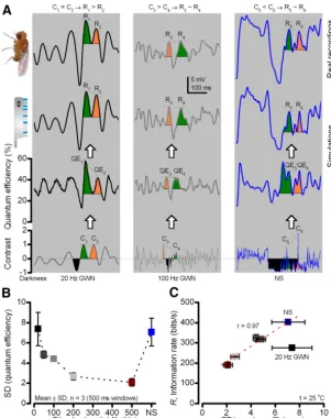
Figure 4. DrosophilaR1–R6 photoreceptors can sample more information from NS than from GWN stimuli.A, Schematic of recording R1–R6 photoreceptors’ voltage responses to light stimuli by conventional sharp microelectrodesin vivo.B, Photoreceptors were adapted to a daylight level (⬃106photon/s) before GWN stimulation with peak-to-peak⫾1 (unit) contrast modulation.C, Intracellular voltage responses to unit-contrast GWN stimuli with 20, 50, 100, 200, and 500 Hz cutoffs. Narrow-band (20 Hz) GWN evokes the largest responses; broadband (500 Hz) the smallest. Recordings from the same cell: means (colored), individual responses (thin gray).D, Voltage signals (thick) adapt but noise (thin) is unchanged by GWN modulation; power spectra calculated from the difference between individual responses and their mean (signal) for each stimulus.E, SNR of photoreceptor output is the highest during 20 Hz GWN. Broadening GWN bandwidth reduces the maximum but widens reliable response bandwidth (SNR⬎1).F, Broadening GWN bandwidth reduces responses’ information rate; decays from⬃320 to⬃190 bits/s.G, With stimulus information rate,Rinput, increasing steadily with broadening GWN bandwidth, photoreceptors’ encoding efficiency (R/Rinput) decreases exponentially.H, Naturalistic light intensity time series (NS) evokes large
responses; mean and 10 responses.I, Photoreceptors’ SNR to NS (cyan) exceeds that to GWN for all the tested bandwidths.J, In every photoreceptor, information transfer to NS was⬎20% higher than to the maximal GWN stimulation (100 Hz cutoff); mean⫾SD,p⫽4.2⫻10⫺5.K, Photoreceptors encode more efficiently NS than 500 Hz GWN of similar input information rates (⬃3000 bits/s); mean (R/Rinput)⫾SD,p⫽9.4⫻10⫺
8
used: (1) Each bump had a fixed shape; the average of all bumps in the corresponding real stochastic simulation. (2) The bumps were generated after a predetermined stochastic latency, which followed the same latency distribution generated by the stochastic phototransduction cascade model. (3) The refractory period was set to 0 ms, although no bumps were allowed to emerge in the middle of an ongoing bump response. (4) The macroscopic response was generated by summing all 30,000 bump series, representing simultaneous outputs of all individual microvilli. For both models (with and without the refractory periods), to eliminate the role of bump shapes, the bump counts were obtained by counting the number of bumps at each time point across the 30,000 microvilli.
Mock stochastic model with bump refractory periods taken randomly from the real distribution. These procedures and assumptions were used (seeFig. 10B,C, Random): (1) Each bump had a fixed shape; the average of all bumps in the real stochastic simulation at the bright light level (105 photon/s). (2) The bumps were generated after a predetermined stochas-tic latency, which followed the latency distribution of the stochasstochas-tic pho-totransduction cascade model. (3) No bumps were allowed to emerge in the middle of an ongoing bump response or during its refractory period. (4) The refractory periods were generated for the same predefined distri-bution, obtained from the real stochastic simulations. (5) The macro-scopic response summed all bump series. By having latencies and refractory period drawn from a predefined distribution, these parame-ters are randomly shuffled along time, and hence eliminate any long-term light-adaption in these parameters (information carried by memory of past events in the real stochastic simulations).
Microvilli usage. To compare how different stimuli used microvilli over time, we calculated the microvilli usage from the mock bump integration model (seeFig. 10D). The light inputs were 2 s of 20, 50, 100, 200, and 500 Hz GWN and NS. In all cases, the photon input to each microvillus was gener-ated by the random photon absorption model (Song et al., 2012).
In the mock stochastic model simulations, all bump parameters and their corresponding distributions were obtained from real stochastic simulations at 105photon/s. The following procedures and assumptions were used: (1) Each bump had a fixed shape (the average of all bumps in the corresponding stochastic simulation). (2) The bumps were generated after a predetermined stochastic latency, drawn from the same latency distribution generated by the stochastic phototransduction cascade model. (3) No bumps were allowed to emerge in the middle of an ongo-ing bump response or durongo-ing its refractory period. (4) The refractory periods were generated for the same predefined distribution, obtained from the corresponding stochastic simulations. (5) The macroscopic re-sponse was generated by summing all bump series. (6) The output state of each microvillus (e.g., generating a bump, refractory) was counted at each 1 ms time bin. This procedure was repeated across 30,000 microvilli to obtain their usage dynamics.
Estimating ATP consumption for information transmission in Drosoph-ilaphotoreceptors.While the microvilli, which form the photosensitive part of aDrosophilaphotoreceptor (Fig. 1), generate the LIC, the photo-insensitive part of the plasma membrane uses many voltage-gated ion channels to adjust the LIC-driven voltage responses. In response to LIC, these open and close, regulating the ionic flow across the plasma membrane. But to maintain the desired ionic concentrations inside and outside, photo-receptors depend upon other proteins, such as ion cotransporters, ion ex-changers, and ion pumps, to uptake or expel ions in and out. The work of the pumps in moving ions against their electrochemical gradients consumes energy (ATP). ATP consumption of aDrosophilaphotoreceptor thus much depends upon the ionic flow dynamics through its ion channels (Laughlin et al., 1998). To approximate these dynamics during light responses, we con-structed a HH model of the photoreceptor body. This electrical circuit mod-els the ion channmod-els as conductances.
Our HH model included these ion transporters: 3Na⫹/2K⫹-pump, 3Na⫹/Ca2⫹-exchanger and Na⫹/K⫹/2Cl⫺mechanisms to balance the intracellular ionic fluxes. Na⫹/K⫹/2Cl⫺cotransporter balances with the voltage-dependent Cl⫺and Cl⫺leak conductances, maintaining intra-cellular Cl⫺concentration. Ca2⫹influx in the LIC (⬃41%) is then ex-pelled by 3Na⫹/Ca2⫹-exchanger in 1:3 ratio in exchange for Na⫹ions. Although there is K⫹influx in LIC (⬃24%), this is not enough to com-pensate K⫹leakage through voltage-gated K⫹conductances and K⫹
leaks. Apart from a small amount of K⫹intake through Na⫹/K⫹ /2Cl-⫺cotransporter, 3Na⫹/2K⫹-pump is the major K⫹uptake mechanism. It consumes 1 ATP molecule to uptake 2 K⫹ions and extrudes 3 Na⫹ ions. Because it is the major energy consumer in the cell, we use only the pump current (Ip) to estimate the ATP consumption.
From the equilibrium of K⫹fluxes,Ipcan be calculated as follows:
Ip⫽
1
2共Ishaker⫹Ishab⫹Inew⫹IKleak⫺ILIC_K兲⫺
1
4共Icl⫹Icleak兲
(6)
whereIshaker,Ishab,Inew, andIKleakare the currents through shaker, shab,
new, and Kleakchannels, respectively,ILIC_Kis the K⫹influx in LIC and
IClandICleakare the currents through the voltage-gated Cl⫺and Cl⫺leak
channels, respectively. These currents can be calculated from the reverse potential of individual ions and their HH model produced conductances using Ohm’s law:
Ishaker⫽共Em⫺Ek兲gshaker (7)
Ishab⫽共Em⫺Ek兲gshab
Inew⫽共Em⫺Ek兲gnew
IKleak⫽共Em⫺Ek兲gKleak
Icl⫽共Em⫺Ecl兲gcl
Icleak⫽共Em⫺Ecl兲gcleak
UsingIp, the number of ATP molecules hydrolyzed per second can be
calculated:
ATP molecules s⫺1⫽
冕
0T
Ipdt
T ⫻
NA
F (8)
whereNAis Avogadro’s constant andFis Faraday’s constant. The
num-ber of ATP molecules per bit of information was calculated by dividing the estimated number of ATP molecules hydrolyzed in a second by the estimated information transfer rates (bits/s).
We did not model the dynamics of these pump mechanisms because, for the purpose of calculating ATP, only the time-integrated ionic fluxes count, not the time constants.
Previously, because of lack of a complete model for the photosensitive membrane, the LIC has only been estimated at the steady state (Laughlin et al., 1998;Niven et al., 2007), when the sum of all currents across the model membrane equals zero:
Ishaker⫹Ishab⫹Inew⫹IKleak⫹Icleak⫹Icl⫹Ip⫹ILIC⫽0 (9)
Because we estimated LIC directly from the stochastic phototransduc-tion model (above), we could calculate a photoreceptor’s energy cost in response to any arbitrary light pattern, including naturalistic stimulation (Table 4). Thus, our phototransduction cascade model provides the functional equivalence to the light-dependent conductance used in the previously published models (Laughlin et al., 1998;Niven et al., 2007).
Results
pathway to the fly brain (Joesch et al., 2010;Wardill et al., 2012). Thus, they constrain how well and fast a fly can see.
Encoding efficiency decreases with broadening stimulus bandwidth
In each experiment, a photoreceptor was adapted to the same daylight level before starting unit-contrast GWN modulation (Fig. 4B), in which frequency range was low-pass filtered to 20, 50, 100, 200, and 500 Hz, while its amplitude range was flanked by contrasts of 1 (twice the mean) and⫺1 (darkness). This gave each stimulus the average contrast of⬃0.32. Theoretically, each of these light intensity time series is maximum entropy among stim-uli with the same bandwidth and variance. Because light emission from the source can be modeled by Poisson statistics, we could calculate from photon fluctuation estimates their input informa-tion rates during repetitive stimulainforma-tion (Fig. 2A–D;Table 1; see Materials and Methods). Then, the encoding efficiency of photo-receptors (their recorded outputs) could be assessed as the ratio between the corresponding output and input information rates (R/Rinput) for each stimulus.
Intracellular recordings (Fig. 4C) showed that the narrow bandwidth stimulus (20 Hz cutoff) evoked the largest responses, whereas broadening the bandwidth reduced the responses. The effect was similar to that caused by increasing the playback veloc-ity of GWN stimulation (Juusola and de Polavieja, 2003), imply-ing that, when the stimulus bandwidth exceeded that of the responses (27.8⫾1.0 Hz half-maximum cutoff, mean⫾SD, 4 photoreceptors), more of its information allocated (i.e., was wasted on) frequencies too fast for the fly to see. This, however, did not affect voltage noise (Juusola et al., 1994) (Fig. 4D), which mostly reflects the average quantum bump (sample) size that integrates the mean responses (Juusola and Hardie, 2001a). Consequently, the mean re-sponse (signal;Fig. 4D) and SNR diminished with the broadening bandwidth (Fig. 4E), although, with too narrow a bandwidth, the stimulus lacked higher-frequency information that the fly eye can process and transmit (Zheng et al., 2006;Wardill et al., 2012). There-fore, these findings could much explain why photoreceptors’ infor-mation transfer rate (Fig. 4F) first rose to⬃320 bits/s at 100 Hz stimulus cutoff (where GWN encoding was maximal) before falling to⬃190 bits/s at 500 Hz cutoff.
Information in GWN stimulation (Rinput) increases steadily with broadening bandwidth (Fig. 4G, light gray). Interestingly, however, photoreceptors’ encoding efficiency (R/Rinput; black)
neither reached a peak along their information capture of 50 –100 Hz GWN (Fig. 4F, gray squares) nor plateaued thereabouts, as could happen if their rhabdomeres sampled light changes with a 100% photon-to-bump conversion rate (quantum efficiency).
Instead, photoreceptors’ encoding efficiency decayed exponen-tially with broadening stimulus bandwidth: from 80% to 90% for 20 Hz stimulation to⬃5% for 500 Hz GWN (Fig. 4G, black). These concurrent but opposing trends suggest that quantum ef-ficiency of sampling adapted to the way light information was distributed within the stimulus bandwidth, further contributing to the photoreceptors’ encoding efficiency.
Photoreceptors can sample more information from naturalistic stimuli than GWN
To determine whether the maximum information rate to 100 Hz GWN (Fig. 4F), having minimal temporal correlations, repre-sented photoreceptors’ capacity, or whether their information sampling could increase with input correlations, we examined encoding of naturalistic stimulation (NS).
Neighboring pixels in natural scenes most probably belong to the same object or background, reflecting similar light intensities, whereas object boundaries or edges reflect differently, separating the world into darker and lighter features (Field, 1987;Ratliff et al., 2010). A naturalistic light intensity time series, as a slice across these features, is not random but contain structured asymmetric contrast variations, which correlate strongly and drive photorecep-tor output vigorously (van Hateren, 1997). But NS can also contain less dynamic sequences, such as intensities scanned over a smooth surface; these adapt responses to lower information rates (van Hat-eren and Snippe, 2001). Therefore, we chose a highly variable NS sequence (Fig. 2E, blue) that included large step-like transitions be-tween longer dark and bright contrasts (van Hateren, 1997; (Zheng et al., 2009) for this test. To attribute potential improvements in encoding to the temporal structure (intensity correlations) of the light patterns (contrasts), NS stimulation was scaled to have the same mean daylight intensity as the GWN.
The given NS sequence (Fig. 4H) consistently evoked large voltage responses with higher SNRs (Fig. 4I) and information transfer rates (Fig. 4J) than the GWN stimuli. The recordings were performed sequentially and occasionally repeated in the same photoreceptor (e.g.,Fig. 4F,Jshows information rates of 7 complete recordings series from 5 cells). Because the responses were highly reproducible, it became evident that the highest in-formation rate estimate (⬃320 bits/s) to GWN stimuli did not represent the capacity, whereas, equally, the higher estimate (⬃400 bits/s) to the NS was unlikely the maximum either. Pre-sumably, there are other light intensity time series, which could evoke responses with even more information. Nonetheless, the findings indicated thatDrosophilaphotoreceptors, overall, en-coded the NS sequence more efficiently than broadband GWNs (200 –500 Hz) of highRinput(Fig. 4K), but less efficiently than
Table 4. Energy usage ofDrosophilaR1-R6 photoreceptors at 25oC when transmitting information about different stimulia
Mean light intensity of the stimulation at microvilli level (105photon/s)
DrosophilaR1-R6 photoreceptor model without refractory period
StochasticDrosophilaR1-R6 photoreceptor model with refractoriness
Information (bits) s⫺1
ATP molecules s⫺1
ATP molecules/bit
Information (bits) s⫺1
ATP molecules s⫺1
ATP molecules/bit
NS 455 7.538⫻109 1.657⫻107 403 4.633⫻109 1.150⫻107 GWN 20 Hz 271 5.261⫻109 1.941⫻107 267 2.999⫻109 1.123⫻107 GWN 50 Hz 356 5.269⫻109 1.480⫻107 319 3.013⫻109 0.945⫻107 GWN 100 Hz 364 5.265⫻109 1.446⫻107 325 3.014⫻109 0.927⫻107 GWN 200 Hz 282 5.275⫻109 1.871⫻107 231 3.017⫻109b 1.306⫻107b GWN 500 Hz 242 5.268⫻109 2.177⫻107 191 3.013⫻109b 1.577⫻107b aMean information transfer rate estimates and corresponding energy expenditure for naturalistic light intensity time series, NS, and unit-contrast GWN, with different cut-off frequencies at the mean illumination of 105photon/s. The middle columns indicate the information rates and energy consumption of the photoreceptor model without a refractory period; the right columns summarize the information and energy for the stochastic photoreceptor model. Stochastically operating microvilli reduce energy consumption on average by⬃42% and ATP/bit by⬃35%.
narrow-band GWN stimuli (20 –100 Hz) of lowerRinput(Fig. 4G). Specifically, encoding ofⱕ50 Hz GWN was submaximal because even their input information rates (Table 1) were below or about what photoreceptors can (or are expected to) sample from information-rich NS (Fig. 4J), whereas encoding ofⱖ200 Hz GWN was inefficient (Fig. 4K) because much of this information was inaccessible to photoreceptors, too fast to be sampled reliably.
To confirm that these encoding characteristics were indepen-dent of the ambient recording conditions, we also performed the experiments in flies with ⬃5°C lower head temperatures (⬃20°C) (Tables 2and3). Predictably, because of more sluggish phototransduction reactions in cooler photoreceptors (Juusola and Hardie, 2001b), responses were slower and their information transfer rates and encoding efficiencies lower (Juusola and Har-die, 2001b) than at the flies’ preferred temperature (Sayeed and Benzer, 1996) of 25°C (Fig. 4). However, the photoreceptors’ information capture from naturalistic stimulation was again higher than that from GWN stimuli by the same margins (NS:
⬃300 bits/s; GWN:⬃220 bits/s).
Encoding retains sensitivity to highly-structured local contrast changes
To what degree does photoreceptors’ high information capture from NS reflect the immediate time order of light intensities (lo-cal contrast changes) rather than their global amplitude or fre-quency distributions? To explore this question, which is about efficiency of information sampling over different time scales, we added two different light intensity time series of equal means to the stimulation regimen. In addition to NS (Fig. 2E, blue), we
now recorded responses to a stimulus (green) that had a random-ized time order of NS intensities (decorrelated; spectrally “white”;Fig. 2G) but the same distribution. We also recorded responses to a Gaussian stimulus (Fig. 2F, orange), in which “pink” (1/f) frequency distribution (Fig. 2G) approximated that of NS. These three distinctive stimuli were presented successively to each tested photoreceptor. Our aim, through comparative quantitative analysis, was then to link differences in encoding (these stimuli) to differences in (their) information allocation.
We discovered that the responses (Fig. 5A) to the original NS (blue) were larger than those to the shuffled (green) or “pink” stimuli (orange). Again, all the responses had similar noise power (Fig. 5B), indicating equivalent average bump (sample) size, as expected after adaptation to the same mean intensity (compare GWN experiments above) (Juusola and Hardie, 2001a). But be-cause the signal (average response) power and thus SNRs (Fig. 5C) were lower in responses to shuffled-NS and Gaussian-1/f stimuli, photoreceptors sampled less information from them. The respective information transfer rates were⬃74% (286 bits/s;
Fig. 5D) and⬃78% (301 bits/s) of that to NS (386 bits/s), and these relationships remained the same also at 20°C (Tables 2and
3). Hence, once photoreceptors adapted to stimulus repetition, the fine time course of light intensity fluctuations (local contrast changes) largely determined their high information capture, with sampling being less sensitive to the global amplitude distribution. Unsurprisingly, the encoding efficiency to shuffled-NS, which had the highest information content but minimal correlations between successive intensity values, much like GWN, was only 7%, half of that to NS (Fig. 5E). Shuffling reduced especially the conspicuous longer intensity fluctuations (phasic or “edge-like”
Figure 5. DrosophilaR1–R6 photoreceptors’ responses to naturalistic light intensity time series (NS, blue) are larger and carry more information than responses of the same cells to shuffled-NS (green) or Gaussian 1/f (orange) intensity series.A, Means (thick) and SD (thin) of intracellularly recorded voltage responses to the repeated stimuli. Each stimulus had the same mean light intensity (106photons/s).B, Signal (average response) power to NS is larger than to shuffled-NS or Gaussian-1/f stimuli, but their noise powers are similar.C, SNR of the responses is the highest to NS and the lowest to shuffled-NS.D, Accordingly, the information rate of the responses is the greatest to NS (**p⫽2.0 –3.8⫻10⫺2). Different lines indicate individual recordings from the same cells.
contrast changes) that evoked the largest responses to NS. In-stead, by now flipping (too) fast between intensities, much of this stimulus information became invisible to photoreceptors, akin to high-frequency GWN. More surprisingly, however, we found that the encoding efficiency to NS and Gaussian-1/f stimuli was approximately the same (⬃15%), despite their different mean contrasts (Fig. 2E,F) and information contents (Fig. 2I). This implies that, while adapting to 1/f frequency distribution of the stimuli, photoreceptors retain sensitivity to the most representa-tive contrast changes, lasting⬃ⱖ30 ms (Fig. 5A–C; 2–30 Hz stimulus frequencies).
These findings, together with the results from the broadband GWN stimulation trials (Fig. 4J,K), imply thatDrosophila photore-ceptors can sample more visual information from the more-structured (“bursty” or “phasic”) high-contrast changes of appropriate dura-tion than from decorrelated or symmetric (Gaussian) contrast dis-tributions. Thus, GWN, shuffled-NS, or Gaussian-1/f stimulation, regardless of their bandwidth and amplitude modulation and the retina temperature, underestimates the potential information ca-pacity of photoreceptors, which can encode more information from natural-like light intensity fluctuations.
Stochastic photoreceptor model encodes realistically
What is the biophysical basis for these encoding differences? Why did Gaussian or decorrelated light inputs of high information content (Fig. 2I) cause clearly submaximal neural output? To gain mechanistic insight into these open questions, we needed to understand how the different stimuli were sampled and pro-cessed at the level of microvilli. Therefore, we first applied the recently established stochasticDrosophilaphotoreceptor model (Song et al., 2012) to simulate responses for the stimuli used in the recordings. The model integrated quantum bumps from 30,000 microvilli to macroscopic LIC (Fig. 6A). This was con-verted to voltage responses through a HH-type cell body mem-brane model (Fig. 6B) (Va¨ha¨so¨yrinki et al., 2006; Song et al., 2012), which also regulated the electromotive force for the light-sensitive current across all microvilli, similar to real cells. The bump latency and waveform dynamics were adjusted by those of the mean adapted photoreceptors (Juusola and Hardie, 2001a;
Song et al., 2012), with free parameters fixed (Song et al., 2012). The simulated voltage responses (Fig. 6C) to the band-limited GWN stimuli closely matched the real recordings (Fig. 4C), showing similar dynamics with the estimated noise power, SNR, and information transfer rate (Fig. 6D–F), suggesting equivalent encoding. Differences were minor and predictable, mostly attrib-utable to the missing recording noise, microsaccadic eye move-ments, long-term adaptation, and intracellular pupil mechanism that dynamically limits photon influx to microvilli (Song et al., 2012), making the simulations proportionally less noisy at lower frequencies (Figs. 4Dand6D). The simulations further lacked information fed via feedback synapses and gap junctions from the neighboring cells (Zheng et al., 2006;Wardill et al., 2012). These extra inputs likely broadened the bandwidth in real recordings, particularly to 20 Hz GWN (Figs. 4Hand6H, thin red lines).
Nonetheless, most importantly for this analysis, the model output to naturalistic stimulation (Figs. 6Hand7A, blue) differed as predicted from those to GWN, shuffled-NS (Fig. 7A, green) and Gaussian-1/f stimuli (Fig. 7A, orange), closely following the behavior of the real recordingsin vivo(Figs. 4and5). Aptly, the simulated responses to NS had a higher signal power, SNR and information transfer rate than to the other stimuli (Fig. 6I,J: GWN;Fig. 7B–D: shuffled-NS and Gaussian-1/f), whereas the noise powers of the simulations showed virtually identical
fre-quency distributions, as expected for the same mean intensity stimuli (Juusola and Hardie, 2001a) (Figs. 6Dand7B). Further-more, for the tested high-input information stimuli (Fig. 2I), the simulations had the highest encoding efficiency with NS (Fig. 7E), which evoked the largest response fluctuations.Tables 2and
3show these correspondences at 20°C.
Information increases with sample rate modulation
Because the stochastic photoreceptor model sampled and pro-cessed light information much like its real counterparts, we could assess with simulations the contribution of microvilli refractori-ness to the observed differences in encoding. We did this system-atically by comparing, for GWN stimuli and NS, the bump (sample) counts of the stochastic model (Fig. 8B) to the bump counts of a deterministic model (Fig. 8A). In the stochastic model, refractory microvilli cannot produce bumps; whereas in the deterministic model, microvilli had no refractoriness, con-verting practically every absorbed photon to a bump. In the sim-ulations, the inputs (photon counts) to the two models were identical and the bumps (outputs) generated by their 30,000 mi-crovilli had the same average shape and latency distribution (see Materials and Methods). Therefore, the synchronized ratios be-tween the model outputs (their bump counts) should provide us unique but representative dynamic quantum efficiency estimates for each stimulus (Fig. 8C).
At bright illumination, many stochastically operating mi-crovilli failed to respond to photons because photons arrived/ were absorbed during the refractory period. This fall in quantum efficiency (Fig. 8C; bump-to-photon ratio) reduced dramatically the overall sample count (Fig. 8B), here by⬃65%. Importantly, the simulations revealed that the diminishing information trans-fer rates with broadening GWN bandwidth (Figs. 4F and6F) resulted from diminishing bump fluctuations, henceforth called sample rate modulation. This was caused by the diminishing con-trast visible toDrosophilaand further modulated by the fall and fluctuations in quantum efficiency (Fig. 8C). Nonetheless, the average sample rate to the different bandwidth GWN stimuli remained the same (Fig. 8B, red dotted line). Thus, with the bumps to different GWN being of the same average size (Juusola et al., 1994;Juusola and Hardie, 2001a) (Fig. 6D), the smallest output modulation to 500 Hz GWN simply comprised the fewest bumps (Fig. 8B, wine). As the photoreceptor membrane affects the signal and noise equally during bump integration (Juusola and de Polavieja, 2003;Song et al., 2012) and data processing theorem (Shannon, 1948), the smallest sample rate modulation must have directly contributed to the lowest information transfer rate (Figs. 4Fand6F). At the opposite end of this scale, natural-istic stimulation (blue), which incorporated larger contrast changes in bursty sequences, used microvilli more efficiently. It evoked the largest sample rate modulation (Fig. 8B), causing the highest SNR (Figs. 4Hand6H) and rate of information transfer (Figs. 4Iand6I) in the photoreceptor output.